Initialization phase

In EOA, an initial concentration population is created with uniform randomization, based on the number of particles and dimensions in equation 1. Generation of the initial population in EOA method is important because it affects the search space of iterations.

(1)$$C_i^{initial} = C_{min} + rand_i( {C_{max}-C_{min}} ) \;\;\;\;i = 1, \;2, \;\ldots , \;n, \;$$

$C_i^{initial}$ is the initial position vector of ith particle, C _min and C _max are the dimension boundary limits, rand _i is a randomized variable within the range of [0,1], and n is the population size of particles. Every population particle is evaluated sequentially, and the fitness values are determined.

Equilibrium candidates

Equilibrium state is the global optimum of the problem and C _eq is the final state of the convergence. In EOA, as given in equation 2, there are four best-so-far particles and plus another calculated particle, that is, the average of four particles is identified as equilibrium candidates. Equation 2 is significant because the first four candidates help EOA for better exploration ability while the averaged one helps in exploitation:

(2)$$\vec{C}_{eq, pool} = \{ {{\vec{C}}_{eq( 1 ) }, \;{\vec{C}}_{eq( 2 ) }, \;{\vec{C}}_{eq( 3 ) }, \;{\vec{C}}_{eq( 4 ) }, \;{\vec{C}}_{eq( {ave} ) }} \}.$$

All the particles update their concentration by selecting randomly one among the candidates.

Exponential term

Concentration updating is realized by the exponential term (F) to ensure the EOA has a reasonable balance between exploration and exploitation by using equations 3 and 4.

(3)$$\vec{F} = a_1sign( {\vec{r}-0.5} ) [ {e^{-\vec{\lambda }t}-1} ] , \;$$

(4)$$t = \left({1-\displaystyle{{Iter} \over {Max\_iter}}} \right)^{( {a_2( {Iter/Max\_iter} ) } ) }, \;$$

where t is a function of iteration, a ₁ and a ₁ are constant values used to manage the ability of exploration and exploitation, sign is the direction, r and λ are random vectors, respectively. Recommended values for a ₁ and a ₁ are equal to 2 and 1, respectively.

Generation rate

Equations 5–7 calculate the generation rate term which provides the exact solution by improving the exploitation phase:

(5)$$\vec{G} = \vec{G}_0\vec{F}, \;$$

(6)$$\vec{G}_0 = \overrightarrow {GCP} ( {{\vec{C}}_{eq}-\vec{\lambda }\vec{C}} ) , \;$$

(7)$$\overrightarrow {GCP} = \left\{{\matrix{ {0.5r_1} & {r_2 \ge GP} \cr 0 & {r_2 < GP} \cr } } \right., \;$$

where $\vec{G}_0$ is the initial value, r ₂ and r ₁ are random numbers between 0 and 1, GCP is the generation rate control parameter, GP is the generation probability. A good equilibrium is reached by using GP = 0.5, between exploration and exploitation.

At final, the updating rule of EOA is given in equation 8.

(8)$$\vec{C} = \vec{C}_{eq} + ( {\vec{C}-{\vec{C}}_{eq}} ) \vec{F} + \displaystyle{{\vec{G}} \over {\vec{\lambda }V}}( {1-\vec{F}} ) , \;$$

where V is the unit. The significance of equation 8 can be summed up as follows:

• • The first term is a global optimum candidate, the second and the third terms are control combinations.

• • Second term contributes more to the exploration by taking advantage of the direct difference between a sample particle and an equilibrium candidate.

• • Third term contributes more to exploitation from small variations in concentration.

Figure 1 shows a 1D visualization of working mechanism of the main equation terms. C ₁ − C _eq represents the second term of the final equation and C _eq − λC ₁ represents the third term of the updating rule of EOA.

Fig. 1. One-dimensional visualization of population modifying their positions.

EOA has a memory-saving technique to help every particle keep track of its location in space with its fitness value. This technique adds to the potential of exploitation; however, it can raise the risk of being trapped into a local minimum. Detailed pseudo code of EOA is given in Fig. 2.

Fig. 2. Pseudo code of EOA.

Linear antenna array

The LAA with the 2M isotropic array element is positioned symmetrically in two sections along the x-axis with M elements as illustrated in Fig. 3. The distance between the elements in this array is determined as λ/2. The all-phase excitation weights are set to zero in the antenna array.

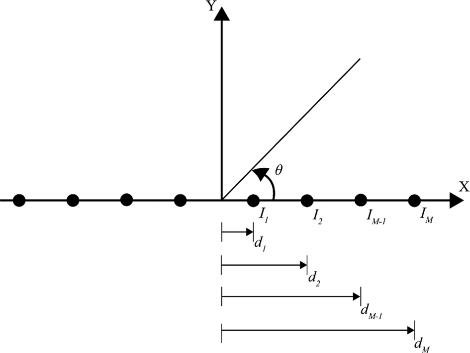
Fig. 3. M-element linear antenna array.

The antenna array factor, given in equation 9, was obtained by assuming that the amplitude coefficients of the array elements are symmetrical around the origin [Reference Balanis1].

(9)$$AF( \theta ) = 2\mathop \sum \limits_{n = 1}^M I_n\cos ( kd_n\sin \theta + \upsilon _n) , \;$$

where I _n and υ_n are the amplitude and phase excitation weight of nth element in the array, respectively. The wave number is k and spacing between the array elements is d. θ is the angle of scanning. The M value here is half the total number of elements in the LAA.

Circular antenna array

Figure 4 illustrates the structure of CAA with M isotropic elements placed non-uniformly on a circle. The radius of the circle placed in the x-y plane is a, and all elements in this structure exhibit similar radiation properties (isotropic source).

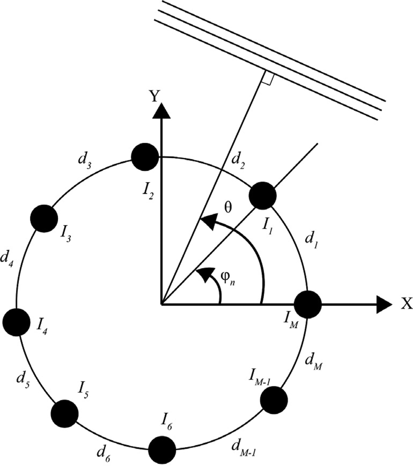
Fig. 4. M-element circular antenna array.

The array pattern of CAA can be defined by its array factor. The CAA's array factor (AF) can be described as in equations 10–13 [Reference Balanis1].

(10)$$AF( \theta ) = \mathop \sum \limits_{n = 1}^M I_n\cdot e^{( {\,j.ka.\cos ( {\theta -\varphi_n} ) + \alpha_n} ) }, \;$$

(11)$$ka = \mathop \sum \limits_{i = 1}^M d_i, \;$$

(12)$$\varphi _n = ( 2\pi \cdot \mathop \sum \limits_{i = 1}^n d_i) /ka, \;$$

(13)$$\;\alpha _n = {-}ka\cdot {\rm cos}( {\theta_0-\varphi_n} ) , \;$$

where α _n and I_n are the phase and excitation amplitude of the nth array element, respectively. d _i is the distance between the two antenna array elements. The number of waves is denoted by k. The nth array element angular position in the x-y plane is denoted by φ _n. The M value indicates the total number of elements of the CAA on the ring.

Cost function formulation

The most important element in antenna array design is the creation of antenna structures that communicate with long distances and are not affected by interference from other communication systems operating in the same frequency band. In order to achieve this, it is necessary to design antenna arrays to obtain radiation patterns with lower MSL and narrower HPBW values. In addition, another important parameter in the application of the antenna design is the physical size of the antenna and this value is desired to be low in designs. The purpose of this article is to determine the position and amplitude values of the array elements by the EOA to obtain the radiation diagram with the lowest MSL and the narrowest HPBW values in order to make optimum antenna design. In order to achieve the optimum antenna synthesis, it is important to design an appropriate cost function to reduce MSL and HPBW. The desired radiation pattern can be obtained by using the cost function given in equation 14.

(14)$$C_{cost} = F_{MSL}\cdot M_{MSL} + F_{HPBW}\cdot M_{HPBW}, \;$$

where F _MSL and F _HPBW are the weight factors. M _MSL and M _HPBW are the functions used to decrease HPBW and suppress the MSL values, respectively. The F _MSL function can be formulated as in equation 15.

(15)$$F_{MSL} = \int_{-\pi }^{\varphi _{n1}} {\mu _{MSL}( \varphi ) \cdot d\varphi } + \int_{\varphi _{n2}}^\pi {\mu _{MSL}( \varphi ) \cdot d\varphi } , \;$$

where φ _n1 and φ _n2 are the two angles at the first nulls on each side of the main beam. μ _MSL(φ) can be given in equation 16.

(16)$$\mu _{MSL}( \varphi ) = \left\{ {\matrix{ {\varepsilon_0( \varphi ) -MSL_d,} & {\varepsilon_0( \varphi ) > \;MSL_d\;\;} \cr {\!\!\!\!\!\!\!\!\!\!\!\!\!\!\!\!\!\!\!\!\!\!\!\!\!\!\!\! 0,} & {\!\!\!\!\!\!\!\!\!\!\!\! \rm elsewhere}}}\right., \;$$

where MSL _d is the desired value of MSL. ɛ ₀(φ) is the array factor in dB. The function M _HPBW can be formulated as in equation 17.

(17)$$M_{HPBW} = \left\{{\matrix{ {M_o-M_{HPBWmax}, }& {M_o > \;M_{HPBWmax}}\cr{\!\!\!\!\!\!\!\!\!\!\!\!\!\!\!\!\!\!\!\!\!\!\!\!\!\!\!\!\!\!\!\!\!\!\!\!0, }& {\!\!\!\!\!\!\!\!\!\!\!\!\!\!\!\!\!\!{\rm elsewhere}}}} \right., \;$$

where M _HPBWmax and M _o are the desired maximum HPBW and the value of HPBW obtained by EOA, respectively.

Optimum design of LAA

In the first example, the amplitudes of the 10-element symmetric LAA are determined by using the EOA method to perform the optimum design. Figure 5 shows the radiation patterns obtained with EOA and other optimization algorithms. The reduced MSL and HPBW values achieved by using EOA, SOS [Reference Dib4], BBO [Reference Sharaqa and Dib5], PSO [Reference Khodier and Al-Aqeel6], Taguchi [Reference Dib, Goudos and Muhsen7], MFO [Reference Das, Mandal, Ghoshal and Kar8], and AFPA [Reference Salgotra, Singh, Saha and Nagar11] are listed in Table 1.

Fig. 5. Array pattern for 10-element LAA design.

Table 1. Comparative results in terms of MSL and HPBW values for 10-element LAA design

The MSL and HPBW values of the array pattern achieved with EOA are −27.01 dB and 12.49°, respectively. As can be clearly seen from Table 1 and Fig. 5, the MSL value of the radiation pattern with EOA is better than the results of other compared algorithms. The HPBW value of EOA is better than MFO and it is very close to the HPBW value of other optimization algorithms.

The number of elements of the LAA is determined as 16 in the second example. The radiation patterns achieved by using EOA, SOS [Reference Dib4], BBO [Reference Sharaqa and Dib5], PSO [Reference Khodier and Al-Aqeel6], Taguchi [Reference Dib, Goudos and Muhsen7], MFO [Reference Das, Mandal, Ghoshal and Kar8], and AFPA [Reference Salgotra, Singh, Saha and Nagar11] are illustrated in Fig. 6. MSL and HPBW values of 16-element LAAs are given in Table 2 comparatively.

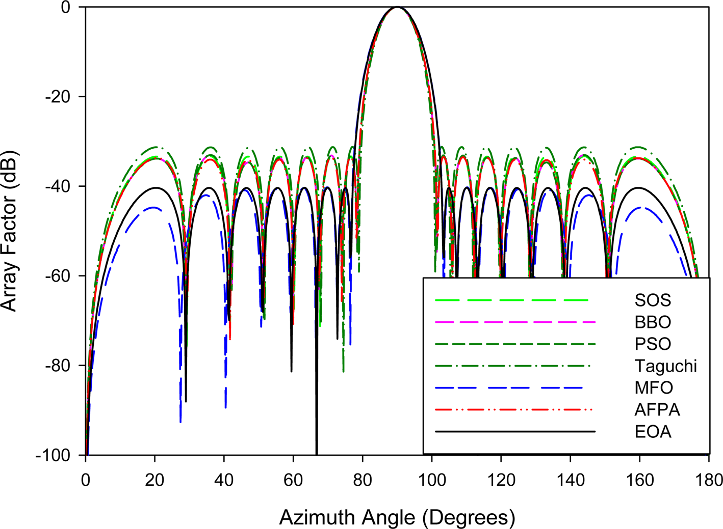
Fig. 6. Array pattern for 16-element LAA design.

Table 2. Comparative results in terms of MSL and HPBW values for 16-element LAA design

It is apparent from Fig. 6 and Table 2, it can be seen that MSL values of radiation pattern obtained by using EOA are better than those of SOS [Reference Dib4], BBO [Reference Sharaqa and Dib5], PSO [Reference Khodier and Al-Aqeel6], Taguchi [Reference Dib, Goudos and Muhsen7], MFO [Reference Das, Mandal, Ghoshal and Kar8], and AFPA [Reference Salgotra, Singh, Saha and Nagar11]. All side lobe levels of the radiation pattern achieved with EOA are lower than −40.35 dB. The HPBW value of EOA method is 8.99°. The results of HPBW values achieved by SOS [Reference Dib4], BBO [Reference Sharaqa and Dib5], PSO [Reference Khodier and Al-Aqeel6], Taguchi [Reference Dib, Goudos and Muhsen7], MFO [Reference Das, Mandal, Ghoshal and Kar8], and AFPA [Reference Salgotra, Singh, Saha and Nagar11] are 8.28°, 8.28°, 8.00°, 8.28°, 9.00°, 8.38°, respectively.

The number of elements chosen is 24 for LAA synthesis in the third example. The array patterns achieved by using EOA, SOS [Reference Dib4], BBO [Reference Sharaqa and Dib5], PSO [Reference Khodier and Al-Aqeel6], Taguchi [Reference Dib, Goudos and Muhsen7], RRA [Reference Subhashini9], and AFPA [Reference Salgotra, Singh, Saha and Nagar11] are plotted in Fig. 7. It is shown in Table 3 that the side lobe levels obtained by the EOA method are suppressed to −41.21 dB and the HPBW is 6°. The results of the SOS [Reference Dib4], BBO [Reference Sharaqa and Dib5], PSO [Reference Khodier and Al-Aqeel6], Taguchi [Reference Dib, Goudos and Muhsen7], RRA [Reference Subhashini9], and AFPA [Reference Salgotra, Singh, Saha and Nagar11] method show the MSL values of −39.37, −37.14, −34.46, 35.02, −41.08, and −37.19 dB, respectively, whereas the HPBW values are 6° for all the cases.

Fig. 7. Array pattern for 24-element LAA design.

Table 3. Comparative results in terms of MSL and HPBW values for 24-element LAA design

The amplitude values of elements optimally determined by using EOA for the synthesis of LAA with 10, 16, and 24 elements are listed in Table 4.

Table 4. The amplitude values of LAA elements using EOA method

Figure 8 shows the converge curve of the LAA with 10, 16, and 24 elements by using EOA. As shown in Fig. 8, 10-element LAA problem converges earlier than those of others due to its low complexity.

Fig. 8. Converge curve of LAA with 10, 16, 24 elements.

Optimum design of circular antenna array

In the optimum design of circular arrays, suppression of MSL plays an important role in preventing undesired interference. In the practical designs of circular arrays, the physical size of the antenna (d_i) is an important parameter and this value is desired to be very small. In addition, it also needs a narrower HPBW value for the circular array to have higher directionality.

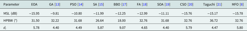
In the second group of examples, first, eight-element CAA synthesis is performed. The radiation pattern obtained by using the EOA method is shown in Fig. 9. For comparison purposes, array patterns obtained by using GA [Reference Panduro, Mendez, Dominguez and Romero13], PSO [Reference Shihab, Najjar and Khodier14], SA [Reference Rattan, Patterh and Sohi15], BBO [Reference Singh and Kamal17], FA [Reference Sharaqa and Dib18], SOA [Reference Guney and Basbug19], CSO [Reference Ram, Mandal, Kar and Ghoshal20], Taguchi [Reference Babayigit and Senyigit21], and MFO [Reference Das, Mandal, Ghoshal and Kar8] are also illustrated in Fig. 9. It is apparent from Fig. 9 and Table 5 that the results achieved by EOA are better than those of GA, PSO, FA, SOA, CSO, Taguchi, and MFO in terms of MSL and HPBW. Although the best values of HPBW are obtained by using SA and BBO, MSL values obtained by these algorithms are quite high for optimum design. The physical size of the antenna is the same in all algorithms except the value of BBO is quite large, which is undesirable for design.

Fig. 9. Array pattern for 8-element CAA design.

Table 5. Comparative results in terms of MSL, d_i, and HPBW values for 8-element CAA design

The optimum design problem of the 10-element CAAs is examined in the second example. The array patterns obtained with EOA and different meta-heuristic optimization algorithms are plotted in Fig. 10. In Table 6, the HPBW, d_i, and MSL values of array pattern achieved by EOA, GA [Reference Panduro, Mendez, Dominguez and Romero13], PSO [Reference Shihab, Najjar and Khodier14], SA [Reference Rattan, Patterh and Sohi15], BBO [Reference Singh and Kamal17], FA [Reference Sharaqa and Dib18], SOA [Reference Guney and Basbug19], CSO [Reference Ram, Mandal, Kar and Ghoshal20], Taguchi [Reference Babayigit and Senyigit21], MFO [Reference Das, Mandal, Ghoshal and Kar8], and CS [Reference Khodier16] are tabulated.

Fig. 10. Array pattern for 10-element CAA design.

Table 6. Comparative results in terms of MSL, d_i, and HPBW values for 10-element CAA design

As can be clearly seen from Table 6 and Fig. 10, MSL and d_i values achieved by the EOA technique are better than the result of other optimization algorithms. The HPBW value achieved by EOA is better than the values found using the MFO methods. The HPBW values of the compared algorithms are less than the value of the proposed method, but if we look in terms of MSL values, it is unacceptably high for an optimum antenna design.

In the last example, the number of elements of the CAA is selected as 12. The array pattern of EOA is compared with those of GA [Reference Panduro, Mendez, Dominguez and Romero13], PSO [Reference Shihab, Najjar and Khodier14], SA [Reference Rattan, Patterh and Sohi15], BBO [Reference Singh and Kamal17], FA [Reference Sharaqa and Dib18], SOA [Reference Guney and Basbug19], CSO [Reference Ram, Mandal, Kar and Ghoshal20], Taguchi [Reference Babayigit and Senyigit21], and MFO [Reference Das, Mandal, Ghoshal and Kar8] in Fig. 11. Table 7 listed the HPBW, d_i, and MSL values of array patterns achieved by EOA and those of GA [Reference Panduro, Mendez, Dominguez and Romero13], PSO [Reference Shihab, Najjar and Khodier14], SA [Reference Rattan, Patterh and Sohi15], BBO [Reference Singh and Kamal17], FA [Reference Sharaqa and Dib18], SOA [Reference Guney and Basbug19], CSO [Reference Ram, Mandal, Kar and Ghoshal20], Taguchi [Reference Babayigit and Senyigit21], and MFO [Reference Das, Mandal, Ghoshal and Kar8].

Table 7. Comparative results in terms of MSL, d_i, and HPBW values for 12-element CAA design

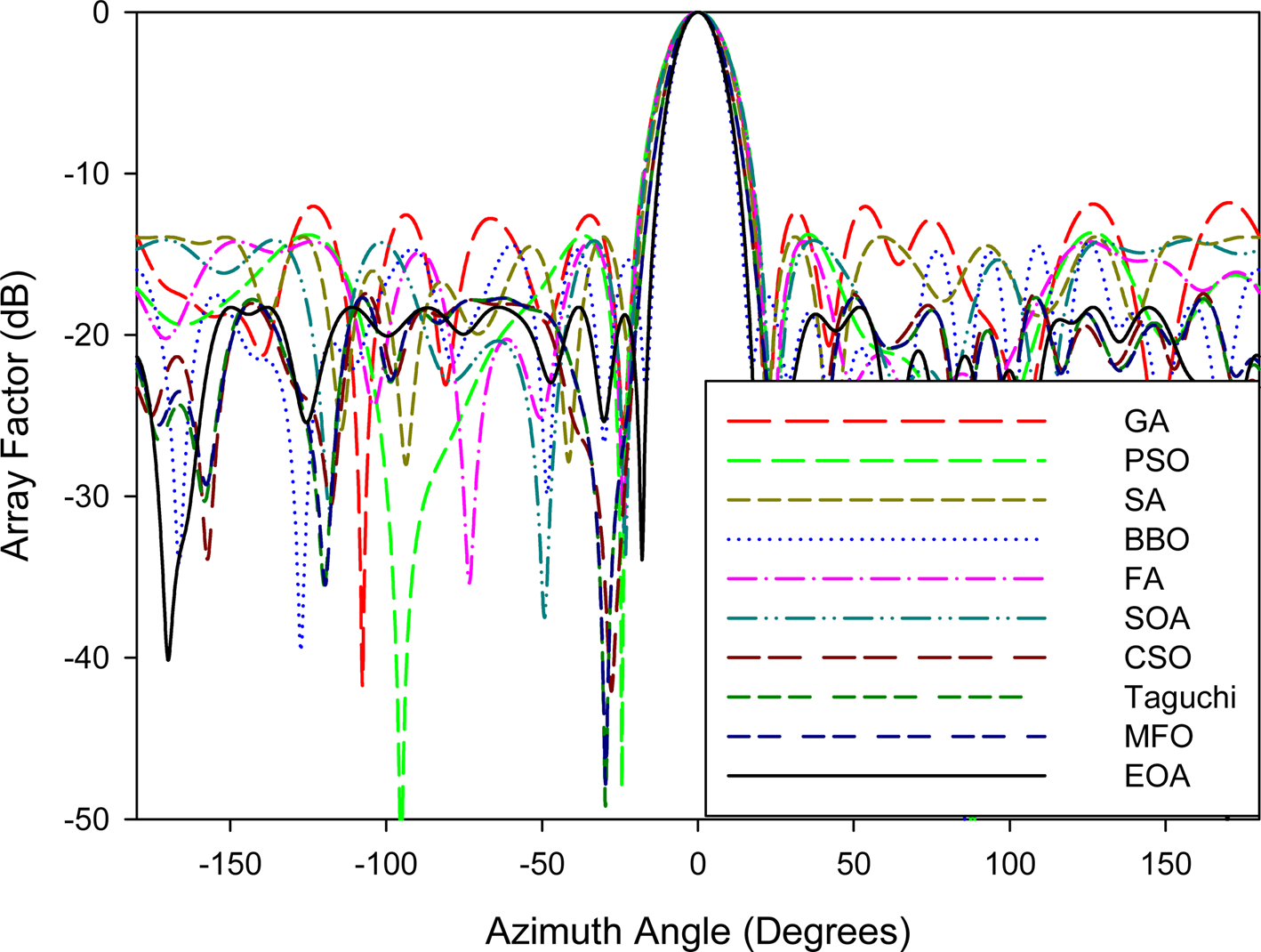
Fig. 11. Array pattern for 12-element CAA design.

From Table 7 and Fig. 11, it is shown that the HPBW and MSL results achieved by EOA are better than the other compared algorithms. If we examine the physical dimensions of the antennas, the antenna obtained with EOA is smaller than the antenna designed with CSO, Taguchi, and MFO.

The position and amplitude values of the elements determined by using EOA for the radiation patterns in Figs 9–11 are tabulated in Table 8. Figure 12 shows the converge curve of the CAA with 8, 10, and 12 elements by using EOA. As shown in Fig. 12, an eight-element CAA problem converges earlier than those of others due to its low complexity.

Table 8. The amplitude and position values of CAA elements using EOA method

Fig. 12. Converge curve of CAA.

The results described in Figs 5–7 and 9–11 illustrate that the proposed method EOA can accurately achieve the optimum radiation patterns of linear and CAAs with lower MSL and equal or narrow HPBW. The HPBW and MSL values of the array patterns obtained with EOA are quite good. The physical size of CAA obtained by EOA is generally better than the other compared optimization algorithms. It can be concluded that EOA can be used as a good alternative to other optimization methods for antenna array synthesis.