


I. INTRODUCTION
The opportunistic radio approach is fundamentally assumed as a flexible system, aware of its immediate environment through sensing operating modes and dynamic reconfiguration properties [Reference Harada1]. Such conditions will offer greatest services and performances to the customer.
The concept of multi-access antennas [Reference El Hajj, Gallée and Person2–Reference El Hajj, Gallée and Person4] is used to exploit the combined flexibility of radio frequency (RF) and digital interfaces, then offering enriched information by combining multi-incoming signals for both transmission/reception modes. The intrinsic performances of the antenna directly affect the software-defined radio (SDR) performances and one challenge lies in the achievement of infinite isolation values between the antenna access ports at different frequencies (bands) (or within the same band). This can be achieved through convenient design and optimization of the radiating structure (shape, excitation, etc.). In this case, a real knowledge and understanding of the antenna operating principles is fundamental and more efficient than a “Cut & Try” method on a commercial electromagnetic (EM) simulator where physical interpretation is often missing.
In this context, the authors in [Reference El Hajj, Gallée and Person2] used stubs to perform the isolation for the bi-access bi-band antenna. In [Reference El Hajj, Gallée and Person3], a new isolation method based on the equivalent cavity modal analysis is developed and illustrated by a bi-access mono-band hexagonal patch antenna. The isolation performance in [Reference El Hajj, Gallée and Person2] is unfortunately quite limited, when considering a stub filtering structure. Indeed, this isolation method (using stub) is only available for a particular case. Although the isolation method in [Reference El Hajj, Gallée and Person3] is more general, the realized antenna has only one band. In [Reference El Hajj, Gallée and Person4], the bi-access tri-band antenna was presented without the details of the analysis method of the cavity approach.
The difficulty in multi-access antennas is in the location choice of the excitation ports to ensure simultaneously isolation and matching conditions. Indeed, by placing the access ports before any modal analysis of a structure, the modes of this latter are forced and other modes may not appear. Accordingly, these ports may excite the same mode and are therefore not isolated. Thus, modes identification in a structure is necessary before any excitation. If a radiation structure can be treated as an equivalent cavity, it will be possible to identify its eigenmodes without any excitation. Physically, the approach is similar to characteristic modes analysis for conductive bodies [Reference Cabedo-Fabres, Antonino-Daviu, Valero-Nogueira and Bataller5, Reference Harrington and Mautz6] that use another mathematical model to find the eigenmodes. Referring to [Reference Cabedo-Fabres, Antonino-Daviu, Valero-Nogueira and Bataller5, Reference Harrington and Mautz6], eigenmodes are independent of any kind of excitation; they only depend on the shape and electrical/physical size of the structure. This idea is used in our cavity approach.
The equivalent cavity approach exists only for some structures. Microstrip antennas are an example. They can be assumed as dielectric loaded cavities, so that the normalized field within the dielectric substrate can be determined by considering this region as a cavity delimited by perfect electric (top and bottom metallization levels) and magnetic (perimeters of the metallization parts) walls. However, these structures (microstrip antenna) have limitations in terms of bandwidth and in terms of modes having performance in radiation. These limits reduce their use in their traditional form in opportunistic multi-access architecture.
In this paper, an extension to different antenna topologies of the cavity principle (considering either slots or short-circuited configurations) is performed and studied. From one part, this cavity approach permits the identification of a design methodology. From the other part, it permits the isolation between antenna accesses through a complete analysis of eigenmodes in the cavity structure. The fields' configuration of each useful cavity mode, obtained without any excitation, should be exploited to determine the suitable location for each access port that ensures the matching and the isolation vis-à-vis to other access ports.
The approach is applied to realize a bi-access tri-band antenna combining a microstrip antenna (patch) with a short-circuit (SC) pin (which can be compared to a planar inverted f antenna (PIFA) configuration), with two additional apertures (slots) for generating multipath, and consequently multi-resonance conditions. This antenna is called PIFA Patch Slot Antenna (PIPSA) [Reference El Hajj, Gallée and Person4]. The antenna has two ports, with operating frequency bands centered approximately on DCS and UMTS/Wi-Fi standards.
II. MODAL ANALYSIS PRINCIPLE
A) Definition
As a definition, characteristic modes are current modes (eigenmodes) numerically obtained for arbitrary-shaped conductive bodies. These modes provide a physical interpretation of the operating principles and radiation phenomena taking place within the antenna's internal volume. Since characteristic modes are independent of any kind of excitation, they only depend on the shape and electrical/physical size of the metallic structure, then inducing particular boundaries conditions, in accordance with Maxwell's theory [Reference Cabedo-Fabres, Antonino-Daviu, Valero-Nogueira and Bataller5, Reference Harrington and Mautz6]. Microstrip antennas, in addition to their numerous advantages in terms of size, weight, cost, and performances, are well suited for creating multi-modes co-existence. Such antennas can be assumed as dielectric loaded cavities, so that the normalized field within the dielectric substrate can be determined by considering this region as a cavity delimited by perfect electric (top and bottom metallization levels) and magnetic (perimeters of the metallization parts) walls [Reference Balanis7]. Thus, we simplify the complex mathematical formulation of the fundamental multimodal analysis method and we propose a new approach for identifying the resonant modes of the cavity (analytically or numerically) through their current and field distributions.
B) Cavity approach of classical patch
Figure 1 presents the equivalent cavity of the classical rectangular patch with limits condition and axis convention. The metallic element (patch) and the ground plane are considered as electric walls, while the four dielectric surfaces along the patch perimeter are considered as magnetic walls. Since the height of the substrate is very low (h⋘λ where λ is the wavelength within the dielectric), the field variations along the height will be considered constant. In addition, because of the very small substrate height, the fringing of the fields along the edges of the patch is also very small whereby the electric field is nearly normal to the surface of the patch. By the application of the above limit conditions, only TMx field configurations will be considered within the cavity. TMx means that Hx the component (along x) of the magnetic field is always zero (see axis convention of Fig. 1). We have to note that, by considering the walls along the patch as magnetic walls, the cavity model does not take into account the fields fringing. This phenomenon tends to decrease the resonance frequencies when passing from the cavity to the antenna. The amount of fringing can be predicted by using the transmission line model of the patch [Reference Balanis7].

Fig. 1. Equivalent cavity of rectangular patch.
Analytically, the electric and magnetic fields within the cavity can be found using the homogenous wave equation. Numerically, cavity fields' configurations of different modes could be found using the eigenmode solution of HFSS, without any excitation.
As illustration, we present (Table 1) the resonant frequency of the first ten eigenmodes for a patch cavity with characteristics. (ɛ r = 2.2, h = 1.588 mm, W = 118.58 mm, L = 100.45 mm, f r ≈ 1 GHz, and tanδ = 9e−4).
Table 1. Resonance frequency of the first ten eigenmodes.

By this method, we can find, for each mode, the fields and current distributions. As example, we show in Figs 2(a) and 2(b)) the electric field (surface currents) distribution for fundamental modes (TMx001 and TMx010) and the first two even modes (TMx002 and TMx020). Note that for the above structure, the orders of these modes are, respectively (1, 2, 4, and 6) in Table 1.

Fig. 2. (a) E- field configuration in the patch cavity. (b) Surface current.
In fact, the denominated (TMx0n0) modes represent the nth resonance along the L-direction (oy-direction), while (TMx00n) modes represent the nth resonance along the W-direction (oz-direction), where (o) is the origin of the coordinate system.
In this way, and using these distributions, we can control the excitation of each mode. An E-field (respectively H-field) excitation for a mode should be done in a region where the E-field (respectively H-field) is non-zero. If not, this mode will not be excited.
This approach seems obvious for this simple structure. This is due to the fact that the same modes can be analytically calculated. However, when the structure is complex, and the analytical solution become impossible, the use of the above method to determine the modes configurations (numerically) without any excitation becomes useful and even crucial. This will be shown later in this paper. We note that the modal analysis of all below cavities is done using the eigenmodes solution of HFSS, without any excitation. Referring to HFSS on line help (V 13), the resonances of a structure are found by solving the equation (S. x + k 02.T. x = 0), for sets of (k 0, x), one k 0 for every x. Where S and T are matrices that depend on the geometry, the materials and the mesh, x is the electric field solution and k 0 is the free-space wave number. The resonance frequency is found by the equation (f = k 0c/2π) where c is the speed of light.
III. EFFECT OF THE CAVITY DEFORMATION
A) Effect of additional slot
Suppose now that an additional slot is created in the patch, as shown in Fig. 3. This slot is oriented along the width (oz-direction) and perpendicular to the length (oy-direction). The slot is characterized by its position from the edge (a), its length (L f), and its width (e f).

Fig. 3. Patch with an additional slot.
1) LIMIT CONDITIONS AND MODAL ANALYSIS
For this new cavity, the limit conditions of the classical patch are conserved (electric and magnetic walls). However, this added slot should be considered as magnetic wall, to simulate an open circuit. This consideration conserves the physical insight of modes configurations, and permits by this way, the modal analysis of the new cavity without any excitation. The new limit condition is also presented in Fig. 3.
To study the effect of the additional slot, the modal analysis is performed on the same patch of Section II, but with slot characteristics (in mm): (a = 26.23, L f = 40, and e f = 4). The resonance frequencies (f r) of first four eigenmodes are shown in Fig. 4(a). The E-field configurations of modes (1 and 2) are shown in Fig. 4(b). The current distributions of modes (1 and 2) are shown in Fig. 4(c).

Fig. 4. (a) Resonance frequencies of first four modes. (b) E-field configuration in the patch with slot. (c) Surfaces current distributions in the patch with slot.
In comparison with Fig. 2, we can deduce that:
• Because they have the same field and current distributions, the mode 2 of the cavity with slot is the TMx001 mode (width resonance) of the classical patch. This is confirmed by the value of resonance frequency: The resonance frequency value of mode no. 1 in Table 1 (TMx001 mode) is almost equal to the resonance frequency value of mode no. 2 in Fig. 4(a).
• The mode TMx010 of the classical patch does not appear in the cavity with slot. This mode is replaced by another mode (mode 1 in Fig. 4 having different fields and currents). This mode resonates on a lower frequency dependent on the slot characteristics. (The resonance frequency value (1.005 GHz) of mode no. 2 in Table 1 (TMx010 mode) is bigger than the resonance frequency value (0.802 GHz) of mode no. 1 in Fig. 4(a)).
By analogy, a generalization of the approach could be deduced. In fact, all denominated TMx00n modes of the classical patch (resonance along W) are not influenced by the addition of the slot (in this direction), and they conserve almost the same field's configurations, currents distributions and resonance frequencies. However, all denominated TMx0n0 modes of the classical patch (resonance along L) are perturbed by the slot (in this direction); they present a new field's configurations, currents distributions, and a lower resonance frequencies.
Physically, the current directions of all modes (TMx00n modes) that resonate along W are parallel to W (oz oriented). And the current directions of all modes (TMx0n0 modes) that resonate along L are parallel to L (oy oriented). Since the ratio (e f/L) is small the slot here is considered as (oz) oriented (see Fig. 3), i.e. parallel to W and perpendicular to L. As a consequence, this slot affects slightly the current distribution of (TMx00n modes). From the other part, it mostly affects the current distribution of (TMx0n0 modes) and extends its electric path. That is why the resonance frequencies of these modes in the cavity are lower than the classical patch. These later depend on slot characteristics, which we will depict in the subsequent sections.
2) FREQUENCY CONTROL BY SLOT CHARACTERISTICS
After studying fields' distributions, the question is: how slot characteristics affect the resonance frequencies of the modes?
Effect of (Lf): the slot length
To study the effect of the slot length, the initial properties of initial patch are conserved (ɛ r = 2.2, h = 1.588 mm, W = 118.58 mm, L = 100.45 mm, and tanδ = 9e−4). For the slot, we take (a = 0.5 L and e f = 4 mm). With these dimensions, the slot length is varied from 0 to 100 mm with a step of 10 mm. For each value, the modal analysis is performed without any excitation, and with respect to the above limit conditions. The resonance frequencies variations of fundamental modes (TMx001: resonance along W; modified TMx010: resonance along L (with slot effect)) are presented in Fig. 5.

Fig. 5. Variation of resonance frequencies with slot length.
Figure 5 confirms the interpretation of Section III.A.1: the slot does not affect TMx001 mode, its resonance frequency stays almost constant with the variation of slot length. From the other part, when the slot length increases, the electric path of the initial TMx010 mode increases, and therefore the resonance frequency of this mode decreases.
Effect of (a): the slot distance from the edge
To study the effect of the slot distance from edge, the initial properties of initial patch are conserved (ɛ r = 2.2, h = 1.588 mm, W = 118.58 mm, L = 100.45 mm, and tanδ = 9e−4). For the slot, we take (L f = 40 mm and e f = 4 mm). With these dimensions, the slot distance (a) is varied from 2.227 to 98.227 mm with a step of 4.8 mm. For each value, the modal analysis is performed without any excitation, and with respect to the above limit conditions. The resonance frequency variations of fundamental modes (TMx001: resonance along W; modified TMx010: resonance along L (with slot effect)) are shown in Fig. 6.

Fig. 6. Variation of resonance frequencies with slot position.
Figure 6 confirms the interpretation of section III.A.1: the slot does not affect TMx001 mode, its resonance frequency stays almost constant with the variation of slot position. For the modified TMx010 mode, two parts of the curve in Fig. 6 are distinguished (note that 0.5 L = 100.454/2 = 50.227 mm). For (a < 0.5 L), if a increases the resonance frequency decreases. For the values around (a = 0.5 L), the resonant frequency is almost constant. For (a > 0.5 L), if a increases the resonance frequency increases symmetrically. A simple explanation method is done for (a < 0.5 L), the other part (a > 0.5 L) is obtained by symmetry. The electric path of the modified TMx010 mode is shown in Fig. 6. This shows that if a increases the electric path increases and the resonance frequency decreases.
Effect of (ef): the slot width
The initial properties of initial patch are conserved. For the slot, we take (L f = 40 mm and a = 0.5 L). Then, the slot width (e f) is varied from 5 to 25 mm with a step of 5 mm. For each value, the modal analysis is performed without any excitation, and with respect to the above limit conditions. The resonance frequencies variations of fundamental modes (TMx001: resonance along W; modified TMx010: resonance along L (with slot effect)) are shown in Fig. 7.

Fig. 7. Variation of resonance frequencies with slot width.
Figure 7 shows that the resonance frequencies of (TMx010 and TMx001) modes are slightly dependent on the slot width. It also shows that the frequency of modified TMx010 mode decreases slowly with (e f). This effect is similar to the slot length (see Fig. 5), when (e f) increases the electric path increases and the frequency decreases. However, Fig. 7 shows that the frequency of TMx001 mode increases slowly with (e f). Indeed, when (e f) increases, the ratio ((e f)/(L)) increases, and the slot orientation influence in the (oy) direction (see Fig. 3) becomes more powerful and affects the TMx001 mode. Therefore, this later resonates along an effective distance (D eff) slightly smaller than W, with (D < D eff < W) and thus on a slightly bigger frequency (see Fig. 7 – TMx001 mode current distribution for a big (e f) value).
In general, when the above cavity is used as antenna, the variation of slot width affects the imaginary part of the input impedance.
B) Effect of SC
Suppose now that an additional SC pin is added to the patch, as shown in Fig. 8. This SC is characterized by its horizontal position a along L, its vertical position b along W.

Fig. 8. Patch with SC.
1) MODAL ANALYSIS AND SC CHARACTERISTICS (RELATIVE POSITION)
For this new cavity, the limit conditions of the classical patch are conserved (electric and magnetic walls). However, this added SC should be considered as an electric wall.
To study the effect of the SC characteristics, the initial properties of initial patch are conserved (ɛ r = 2.2, h = 1.588 mm, W = 118.58 mm, L = 100.45 mm, and tanδ = 9e−4). For the SC characteristics: we take three cases: I, a = 0.5 L and b = 0; II, a = 0.25 L and b = 0; III, a = 0.25 L and b = 0.25 W. For each case, the modal analysis is performed without any excitation, and with respect to the above limit conditions. The resonance frequencies of the first three eigenmodes in each case are shown in Fig. 9.

Fig. 9. Eigenmodes for each SC case.
To explain these frequency values in comparison with initial cavity (patch), we present in Fig. 10, the E-field configurations and current density distributions of modes 1 and 3, in cases I and III.

Fig. 10. Modes 1 and 3 in cases I and III. (a) Fields distributions. (b) Currents distributions.
• First, the presence of SC creates a new mode that resonates for an electric path corresponding to the quarter of wavelength. This mode is the mode no. 1 in all cases (I, II, and III), it depends on the SC position (i.e. a and b). That is why the resonance frequency of mode 1 in Fig. 9 changes if a or b change. Figure 9 shows that the frequency of this mode increases with a (respectively b), if a < 0.5 L (respectively b < 0.5 W), because in this case the electric path depends on L-a (respectively W-b). By cons, other cases show that the frequency decreases with a (respectively b) if a > 0.5 L (respectively b > 0.5 W), because in this case the electric path depends on a (respectively b). It is the dual phenomenon that is observed in Fig. 6 for the slot position. This mode is the most used and known in PIFA antennas.
• Secondly, to understand the effect of SC on patch modes, the principal idea is: the SC imposes a zero electric field (maximum of current) in the position where it is placed. If this SC is placed in a position where the E-field of the original mode (in the patch without SC) is zero, this SC does not affect this mode, if not this mode is perturbed (i.e. frequency and fields configurations changes). To illustrate this, we take as an example the patch fundamental mode TMx010 (mode no. 2 in Table 1 with field configuration in Fig. 2). In case I of Figs 9 and 10, the SC is placed in an area where the E-field of this mode is zero, that is why the resonance frequency does not change (f ≈ 1.006 GHz for mode no. 2 in Table 1 and for (case I, mode no. 3) in Fig. 9). In Fig. 10 (case I, mode no. 3), this mode conserves the same fields and current distributions. However, in case III, the SC is placed in an area where the E-field of this mode is non-zero, that is why the resonance frequency changes (f = 1.006 GHz for mode no. 2 in Table 1 and f = 1.12 GHz for (case III, mode no. 3) in Fig. 9). In Fig. 10 (case III, mode 3), this mode does not conserve the same fields and current distributions.
All the conclusions of Section III will be used in the design of the bi-access tri-band antenna.
IV. APPLICATION – DESIGN OF A BI-ACCESS TRI-BAND ANTENNA
Suppose now that we want to design an antenna with two isolated accesses and covering three bands, using the previous cavity analysis.
To create a multi-modal co-existence, and therefore increasing the opportunity of the bi-access isolation, two slots and one SC are added simultaneously to the patch. The fundamental structure (antenna considered as a cavity) is shown in Fig. 11. Basically, it is a microstrip antenna (patch) with a SC pin (which can be compared to a PIFA configuration), with two additional radiating apertures (slots). This antenna is called PIPSA.
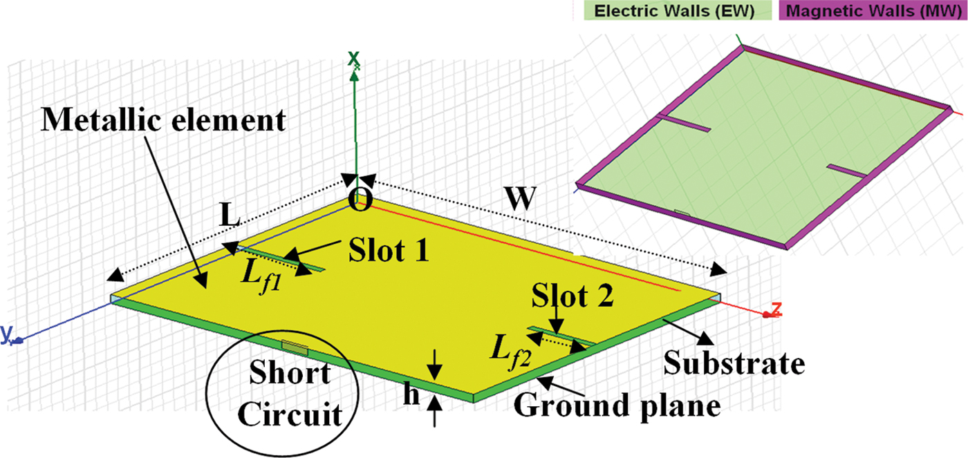
Fig. 11. Basic structure assumed as dielectric-loaded cavity with boundary conditions.
The SC is fixed on a position where a = L and b = 0.5 W. At this position, the E-fields of patch odd modes that resonate in the transversal W-direction, i.e. the denominated TMx00n modes (n is odd) are zero, but not for patch odd modes that resonate in the longitudinal L direction, i.e. the denominated TMx0n0 modes (n odd) (see Fig. 2). Using the analysis of Section III.B.1, this SC perturbs the longitudinal odd modes (TMx0n0) (specially the fundamental TMx010 mode), but not transversal odd modes (TMx00n) (specially the fundamental TMx001 mode).
The slots (in the W-direction) are used to create additional modes without disturbing or influencing the TMx00n modes, these slots being parallel to their current distributions (see Section III.A.1). These slots are fixed at 0.5 L.
Therefore, our design parameters are: L, W, and (L f1, L f2) lengths of the slots (1, 2).
A) Modal analysis and design method
The modal analysis of the above cavity is performed without any excitation using the finite-element method from HFSS™ – Ansoft. Figure 12(a) shows the electric field distribution of the four first resonant eigenmodes, and Fig. 12(b) the corresponding current distributions.

Fig. 12. (a) Electric field distribution (V/m). (b) Current density (A/m).
Referring to Fig. 12(b), the equivalent electric path related to each established resonant mode can be identified (each path is indicated by the corresponding arrow or circle in Fig. 12(b)). Therefore, this understanding approach guides the design methodology; mode 2 (fundamental TMx001 mode of the rectangular patch) depends on the width W, while mode 1 (imposed by the SC condition – see Fig. 11) determines the length L once W fixed. Finally, mode 3 (respectively mode 4) determines the length L f1 of slot 1 (L f2 of slot 2, respectively).
To prove the quasi-independence of the dimensions in modes' frequency control, we show as an example in Fig. 13(a) (respectively Fig. 13(b)) the variation of all modes (1–4) resonance frequencies as a function of the slot 1 length (L f1) between 13.2 and 17.2 mm (respectively, as a function of slot 2 length (L f2) between 8 and 12 mm). Markers in Fig. 13(a) show that for the same variation of L f1, a resonance frequency shift of 8.5% ((2.047–1.873)/2.047 = 0.085) is observed for mode 3 (respectively, 2.8% ((2.387–2.32)/2.387 = 0.028) for mode 4). The resonance frequencies of modes 1 and 2 remain unchanged. This shows that L f1 controls essentially the frequency of mode 3. Markers in Fig. 13(b) show that for a given change in L f2, a resonance frequency shift of 2.15% ((2.05–2.006)/2.05 = 0.0215) is observed for mode 3 (respectively, 7.23% ((2.545–2.361)/2545 = 0.0723) for mode 4). The resonance frequencies of modes 1 and 2 remain unchanged. This shows that L f2 controls essentially the frequency of mode 4. Figure 13 shows that all modes can be controlled independently.

Fig. 13. Effect of slot lengths on modes. (a) Slot 1 and (b) Slot 2.
An example of the obtained resonant frequency of each eigenmode is reported in Table 2 considering our design on a Duroïd™ substrate (ɛ r = 2.2 and thickness (h) = 1.588 mm). Consequently, the perfect understanding and control of each occurring resonating condition for a given eigenmode within the equivalent electromagnetic cavity of the multi-resonance structure leads to accurately control the basic operating frequencies of the antenna.
Table 2. Eigenmodes and corresponding bands for the designed PIPSA.

B) Isolation principle and bi-access operation
1) PORTS LOCATIONS
Two exciting ports are isolated for a given mode if one of them only excites this mode, while the other remains completely electromagnetically transparent. An E-field (respectively, H-field) excitation for a mode should be carried out in a region where the E-field (respectively H-field) is non-zero. If not, this mode will not be excited. Therefore, the results shown in Fig. 12(a) must be exploited for properly identifying the appropriate excitation for each existing mode. For instance, we deduce from such an analysis that the mode 1 with E-fields homogeneously distributed over almost the complete structure cannot be efficiently isolated from other co-existing modes. Consequently, we only exploit modes 2, 3, and 4 for obtaining bi-access operation conditions. Since the current densities of mode 2 from one part and modes 3 and 4) from the other part (Fig. 12(b)) are almost orthogonal (except for the slots locally closed), good isolation level can be easily achieved between mode 2 and modes (3 and 4). We investigate into the various solutions for simultaneously optimizing isolation and return loss performances between these different ports (exciting modes 2, 3, and 4) over the operating frequency bands. Figure 14 shows the 3D E-Field cartography in the structure for the four modes (knowing that mode 1 will not be used for the bi-access operation). These curves were obtained by a hybrid treatment (HFSS and Matlab) that permits the extraction of the field values obtained by cavity analysis of each mode, and then associate it with a point in the structure. By carefully examining the field cartography, we can deduce two lines (L1 and L2) on which the two excitation ports of mode 2 and modes (3 and 4) may be positioned, respectively, to provide simultaneously the isolation and matching conditions. These two lines are shown in Fig. 15.
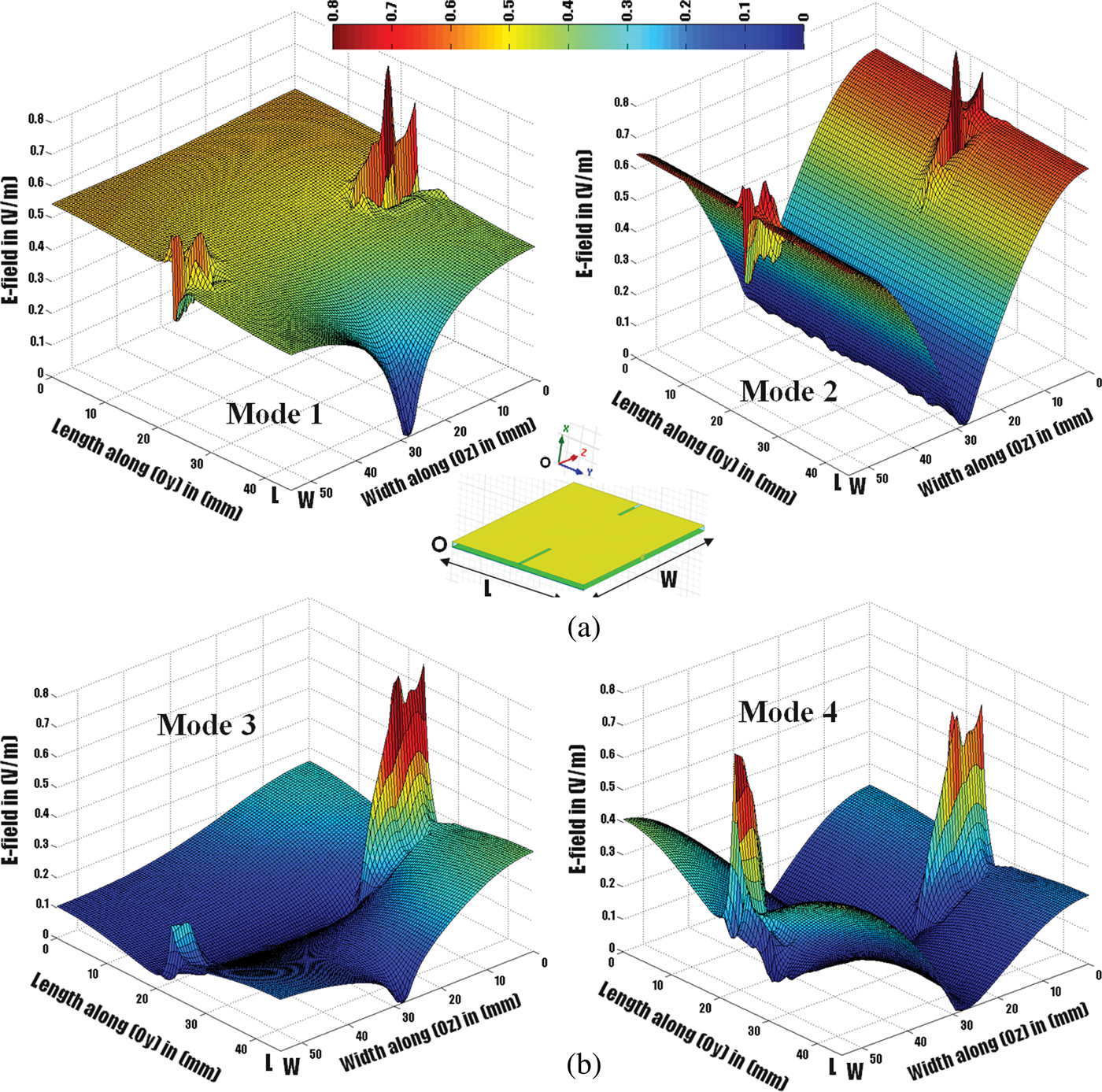
Fig. 14. E-field magnitude for each mode overall structure.

Fig. 15. Determination of the reference lines for exciting specific modes.
On reference lines L1 and L2 (Fig. 15), there are solid and dotted parts. On the solid parts along L1, a non-zero E-field related to mode 2 intersects with zero field related to modes (3 and 4). At the same time, on the solid parts along L2, a non-zero E-field related to modes (3 and 4) intersects with zero field related to mode 2. Thus, the port of mode 2 (modes 3 and 4, respectively) must be along L1 (L2, respectively).
2) PORTS MATCHING
To ensure the impedance matching, we present in Fig. 16 the variation of E-field magnitude versus the normalized distance along L1 (l 1/W) and L2 (l 2/L), where L and W are the dimensions in Fig. 11. The mode 2 is assumed to be the TMx001 mode of a conventional rectangular patch, thus its input impedance at a given point could be deduced analytically using a well-known transmission line model [Reference Derneryd8]. Therefore, for F 2 = 1.8 GHz on a Duroid™ substrate, a 50 Ω matching condition can be ensured for an excitation located at 0.38 W. At this point and referring to Fig. 16(a), the E-field of modes (3 and 4) is almost zero, thus resulting in an intrinsic perfect isolation between mode 2 and modes (3 and 4) excitations.

Fig. 16. E-Field magnitude versus normalized distance L1 (graph (a)) and L2 (graph (b)).
For modes (3 and 4), the matching cannot be analytically determined due to the complex E-field distribution of excited modes. Consequently, considering spatial E-field distributions along L2 from Fig. 16(b), a 50 Ω matching point can be identified for modes (3 and 4) between 0.1 L and 0.3 L along L2. Below 0.1 L, a quite important variation of the E-field magnitude associated with modes 3 and 4 appears, with great difficulty to achieve 50 Ω matching positions for both modes simultaneously. Above 0.3 L, the E-field components for these different modes (2, 3, and 4) have quite similar amplitudes, close to 0, thus corresponding to low-impedance values. Consequently, great difficulties would be encountered for exciting the expected modes (3 and 4) without activating the undesired one (mode 2), due to this co-location and low impedance value constraints. Along L2, the E-field amplitude of mode 2 is almost zero. It will consequently not be excited whatever the location of modes (3 and 4) excitation port.
C) Antenna prototype and measurement
1) S-PARAMETERS
Considering the previous behavioral analysis, a final optimization procedure is carried out on HFSS™ (driven modal solution) for properly controlling the matching, the isolation, and resonating conditions once the E-field excitation ports are considered. Figure 17 shows the antenna prototype on Duroïd™ substrate as well as simulated and measured S parameters. S 11 (S 22) denotes the reflection coefficient at port 1 (2), and S 12 denotes the coefficient of coupling between ports 1 and 2. The dimensions in mm in Fig. 17 are {L = 44.95, W = 54.5, a = 0.38 W (same value of analysis (see Fig. 16(a))), b = 0.5(L + e), c = 0.248 L (well between 0.1 L and 0.3 L (see Fig. 16(b))), d = 0.546 W, e = 1, L f1= 14.2, and L f2 = 10}. In Fig. 17, the excitation port 1 of mode 2 is nominated port M2, and the port 2 of modes (3 and 4) is nominated port M(3 and 4).

Fig. 17. (a) Antenna prototype. (b) Measured and simulated S parameters.
Then 20 MHz and 15 MHz bandwidths (@ROS = 2) are observed in DCS band (port1) and UMTS/ Wi-Fi bands (port 2), respectively, with isolation around 10, 10.4, and 19 dB, respectively. Therefore, we find the predicted bands and the isolation between the two ports, and thus the validation of the design principle (10 dB isolation reference level is considered). For this isolation level (10 dB) and with a reflection coefficient of −10 dB on the port, the antenna conserves 80% of its intrinsic gain (1 − |S11|2 − |S21|2 = 1 − 0.1 − 0.1 = 0.8). We note that the isolation level also depends on the multi-access architecture of the RF front-end and on the reconfiguration algorithms. As we are in an opportunistic cognitive radio context (see acknowledgement), there is no given standard for the multi-access isolation level.
This work is a part of TERROP project (see Acknow ledgement). In this project, a multi-access architecture is used. The fundamental idea is to use many parallel signal paths with discrete time filters, A/D converters, and amplifiers. The intelligent division/recombination of UMTS/ Wi-Fi signals is done via these paths.
2) RADIATION CHARACTERISTICS
The radiation patterns of mode 2 are similar to those of TMx001 mode of a conventional patch, while modes 3 and 4 exhibit approximately radiation patterns similar to those of two equivalent radiating slots of length L f1 and L f2, respectively. The antenna efficiency is greater than 73% over all bands and the maximum gains are 6, 5.6, and 3.45 dBi for modes 2, 3, and 4, respectively. These radiation patterns (simulated) in E and H planes in terms of gains (co and cross polarization) are presented in Figs 18(a)–18(c), respectively, with the new axis convention. Since the current densities of mode are width oriented and that of modes (3 and 4) (Fig. 12(b)) are length oriented (except for the slots locally closed), the E-plane of mode 2 is the H-plane of modes (3 and 4) and vice versa. For modes (3 and 4), the amount of current locally closed around the slot that are oriented toward the width decreases the polarization purity of these modes (Co-Cross ratio in the principle radiation direction is 26 dB for mode 3 and 15 dB for mode 4). For mode 2, all currents are width oriented. The polarization purity of mode 2 is consequently improved (Co-Cross ratio in the principle radiation direction is 40 dB).

Fig. 18. Radiation patterns. (a) Mode 2 [Port M2: excited/Port M(3, 4): 50 Ω]. (b) Mode 3 [Port M2: 50 Ω/Port M(3, 4): excited]. (c) Mode 4 [Port M2: 50 Ω/Port M(3, 4): excited].
V. CONCLUSION
A new approach to modal analysis using equivalent resonant cavity is presented. The modal analysis of initial patch cavity is studied, and then the principle is extended to other topologies containing slots and SC. This approach permits the visualization of fields' configuration without any excitation. This characteristic is very useful when using this cavity as antenna with many access ports; it permits excitement of a given mode(s) in a given location(s), in a manner to ensure the isolation between antenna access ports. In the context of multi-access antenna, there are many advantages of modal analysis compared to brute force parametric optimization. Indeed by using “brute force” parametric optimisation, we force the modes excited in the structure. Therefore, some modes that can be useful are not exploited. From the other part, the isolation between ports will be more difficult because we do not have priori information about modes fields. By using cavity approach (eigenmodes solutions), we can identify and control the modes and their field without excitation, and then we can find the suitable areas to excite a given mode as we had done earlier (Figs 14 and 15). Another advantage is in the time of simulation. The simulation of the above structure on HFSS takes 8 min (480 s) with the classical simulation (driven modal solution). However, with the eigenmodes solution, the simulation of the same structure is done within 30 s. A gain of 16 is obtained in time of simulation. This is due to the fact that the eigenmodes simulation is done without excitation and without the radiation box and because the dimensions of substrate and ground plane are not larger than the metallic element.
As an application, a new antenna for a future opportunistic communication system is presented, with the specific design method proposed for controlling the intrinsic intra-band performances (return loss, excitation, and modes distribution), while enhancing the inter-band isolation. The bandwidth (quite small here) can be improved by inserting complementary modes [Reference El Hajj, Gallée and Person9]. Furthermore, an extension of the method to extra ports, extra bands, and other antenna types is possible. That offers numerous possibilities for identifying generic antenna configurations attractive for SDR, multiple input multiple output (MIMO) or Spectrum-sensing applications.
ACKNOWLEDGEMENT
This work is part of the TERROP project (Opportunistic Radio Terminals) under the financial support of the National Research Agency (ANR) (Inter-Carnot program) in collaboration with Fraunhofer Institutes in Germany.
 Walid El Hajj received his degree in electric and electronic engineering (telecommunication and computer specialty) from the Lebanese University Faculty of Engineering, Beirut-Lebanon, in 2008. He received a National Degree of Master for his Research in “Microwave materials and devices for communication systems” from Telecom Bretagne, Brest–France, in 2008. He received a Ph.D. degree on Information and Communications Sciences and Technologies from Telecom Bretagne, Brest–France in 2011. Since 2011, he is a Research and Development engineer in Lab-STICC/MOM laboratory at Telecom Bretagne.
 François Gallée received the Ph.D. degree in electronics from the University of Brest, Brest, France, in 2001. From 2001 to 2007, he was a research engineer in Antennessa Company. His main activity was antenna design. Currently, he is an Associate Professor with the Microwave Department, Telecom Bretagne/Telecom Institut. He currently conducts research with the LabSTICC. His research concerns the development of new technologies for microwave and millimeter-wave applications and systems.
 Christian Person received the Ph.D. degree in electronics from the University of Brest, Brest, France in 1994. Since 1991, he has been an Assistant Professor with the Microwave Department, Ecole Nationale Supérieure des Télécommunications de Bretagne, Brest, France. In 2003, he became a Professor with the Telecom Institute/Telecom Bretagne, Brest, France, where he currently conducts research with the “Information and Communication Science and Technology Laboratory” (LabSTICC). He is involved in the development of new technologies for Microwave and Millimeter-wave applications and systems. His activities are especially focused on the design of passive functions (filters and couplers) and antennas, providing original solutions in terms of synthesis techniques, analysis, and optimization procedures, as well as technological implementation (Foam, plastic, LTCC, etc.). He is also concerned by RF-integrated Front-ends on Si, and he is currently involved in different research programs dealing with SoC/SiP antennas and reconfigurable structures for smart systems.


