Problem statement

The geometry of a hexagonal array antenna can be developed using two concentric ring arrays of different radius. Figure 1 represents a hexagonal array of 2N isotropic elements placed in the x–y plane. The general array factor expression of a hexagonal array antenna can be given as:

(1)$$AF( \theta , \;\varphi ) = \sum\limits_{n = 1}^{N} \matrix{[ \mathop A\nolimits_n \mathop e\nolimits^{\,jk\mathop r\nolimits_1 \sin \theta ( \cos \mathop \phi \nolimits_{1n} \cos \varphi + \sin \mathop \phi \nolimits_{1n} \sin \varphi ) } \hfill \cr + \mathop B\nolimits_n \mathop e\nolimits^{\,jk\mathop r\nolimits_2 \sin \theta ( \cos \mathop \phi \nolimits_{2n} \cos \varphi + \sin \mathop \phi \nolimits_{2n} \sin \varphi ) } ] , \;\hfill} $$

where A_n represents the excitation current amplitude of the nth element located at the vertices of the hexagonal array and B_n represents the current excitation amplitude of the nth element located in the middle of each arm of the hexagonal array antenna. Here θ is the elevation angle (θ ∈[−π/2, π/2]) and φ is the azimuth angle (φ ∈ [0, 2π]).

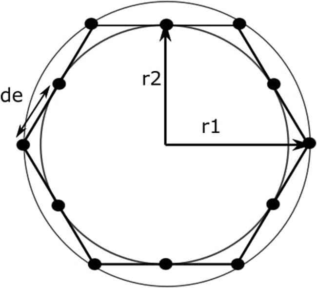
Fig. 1. Hexagonal antenna array.

The circumferential curve of the vertices of the hexagonal array is contrived by a circular array of radius r ₁ and consists of N number of isotropic array elements. The circumferential curve consists of the array elements present in the middle of each arm of the hexagon can be depicted using a circular array of radius r ₂, comprising N isotropic elements. These r ₁ and r ₂ are related as follows:

(2)$$\eqalign{& \mathop r\nolimits_2 = \mathop r\nolimits_1 \times \cos ( {\pi / N}) , \;\cr & \mathop r\nolimits_1 = \mathop d\nolimits_e \times \sin ( {\pi / N}) , \;} $$

where d_e is the inter-element spacing. The angular location of the antennas located at the vertices of the hexagonal array antenna is given as follows:

(3)$$\mathop \phi \nolimits_{1n} = \displaystyle{{2\pi ( N-1) } \over N}.$$

The angular location of the antennas present at the middle of each arm of the hexagonal array is given as follows:

(4)$$\mathop \phi \nolimits_{2n} = \mathop \phi \nolimits_{1n} + \displaystyle{\pi \over N}.$$

In this paper, we have considered a concentric array of hexagonal antennas to reconfigure the beam shaped in the radiation pattern. The geometry of a concentric hexagonal array antenna is shown in Fig. 2. The array factor for M concentric hexagonal array antennas is expressed as

(5)$$AF( \theta , \;\varphi ) = \sum\limits_{m = 1}^{M} {\sum\limits_{n = 1}^N \matrix{[ \mathop A\nolimits_m \mathop e\nolimits^{\,jk\mathop r\nolimits_{1m} \sin \theta ( \cos \mathop \phi \nolimits_{1n} \cos \varphi + \sin \mathop \phi \nolimits_{1n} \sin \varphi ) } \hfill \cr \quad + \mathop B\nolimits_m \mathop e\nolimits^{\,jk\mathop r\nolimits_{2m} \sin \theta ( \cos \mathop \phi \nolimits_{2n} \cos \varphi + \sin \mathop \phi \nolimits_{2n} \sin \varphi ) } ] . \hfill} } $$

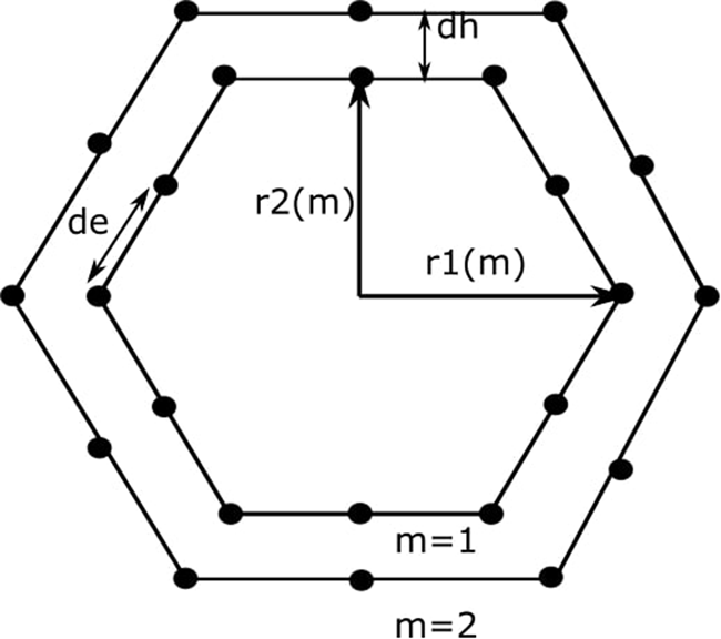
Fig. 2. A concentric hexagonal antenna array.

Each hexagon in the array has a 2N number of isotropic antennas. A_m and B_m are the amplitudes of the excitation current of the elements present at the vertices and the middle of each arm of the mth hexagon, respectively,

(6)$$\eqalign{& \mathop r\nolimits_{1m} = r + ( m-1) \mathop d\nolimits_h , \;\cr & \mathop r\nolimits_{2m} = \mathop r\nolimits_{1m} \times \cos ( {\pi / N}) , \;} $$

where r represents the radius of the outer circle of the innermost hexagon of a hexagonal antenna array.

A hexagonal array antenna with 3N isotropic antennas is shown in Fig. 3. There are one element in each vertex and two elements in each arm. The array factor can be expressed as

(5)$$AF( \theta , \;\varphi ) = \sum\limits_{m = 1}^{M} {\sum\limits_{n = 1}^N \matrix{[ \mathop A\nolimits_n \mathop e\nolimits^{\,jk\mathop r\nolimits_{1} \sin \theta ( \cos \mathop \phi \nolimits_{1n} \cos \varphi + \sin \mathop \phi \nolimits_{1n} \sin \varphi ) } \hfill \cr + \mathop B\nolimits_n \mathop e\nolimits^{\,jk\mathop r\nolimits_{2} \sin \theta ( \cos \mathop \phi \nolimits_{2n} \cos \varphi + \sin \mathop \phi \nolimits_{2n} \sin \varphi ) } \cr \quad + \mathop C\nolimits_n \mathop e\nolimits^{\,jk\mathop r\nolimits_{3} \sin \theta ( \cos \mathop \phi \nolimits_{3n} \cos \varphi + \sin \mathop \phi \nolimits_{3n} \sin \varphi ) } ] . \hfill} } $$

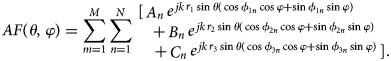
where C_n is the amplitude of the element having the radial distance r ₃. r ₂ and r ₃ represent the radial distance of the antennas present in each arm and r ₁ represents the radial distance of the elements present at the vertices of the hexagon, as shown in Fig. 3.

(8)$$\eqalign{& \mathop r\nolimits_3 = \sqrt 3 \times \mathop {( d}\nolimits_e /\sin ( \mathop \phi \nolimits_{3n} ) ) , \;\cr & \mathop r\nolimits_2 = \sqrt 3 /2 \times \mathop {( d}\nolimits_e /\sin ( \mathop \phi \nolimits_{2n} ) ) , \;\cr & \mathop r\nolimits_1 = \mathop d\nolimits_e \times \sin ( {\pi / N}) , \;} $$

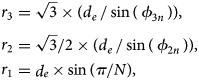
where d_e is the inter-element spacing and $\mathop \phi \nolimits_{2n}$, $\mathop \phi \nolimits_{3n}$are the angular positions of the elements present in each arm, calculated from the positive x-axis, as shown in Fig. 3. These values can be obtained using the equations below:

(9)$$\eqalign{& \mathop \phi \nolimits_{3n} = \mathop \phi \nolimits_{1n} + \mathop {\tan }\nolimits^{{-}1} ( \sqrt 3 /( ( r/) -1) ) , \;\cr & \mathop \phi \nolimits_{2n} = \mathop \phi \nolimits_{1n} + \mathop {\tan }\nolimits^{{-}1} ( \sqrt 3 /( ( 2 \times r/\mathop d\nolimits_e ) -1) ) , \;\cr & \mathop \phi \nolimits_{1n} = 2\pi ( n-1) /N.} $$

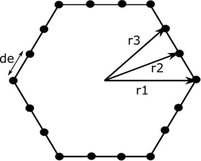
Fig. 3. 18-Element uniform hexagonal array antenna.

The normalized far-field radiation pattern in dB can be expressed as

(10)$$\mathop {AF}\nolimits_{norm} = 20\mathop {\log }\nolimits_{10} \left[{\displaystyle{{\vert {AF( \theta , \;\varphi ) } \vert } \over {{\vert {AF( \theta , \;\varphi ) } \vert }_{\max }}}} \right].$$

To generate reconfigurable beam patterns, we need to achieve the best common excitation current amplitude distribution across the radius of the hexagons using meta-heuristic algorithms. The current amplitudes for all the elements, A_m and B_m are kept between 0 and 1 and varied across the radius of the hexagon of the hexagonal array antenna. Moreover, a smooth amplitude distribution with lower variation is targeted to achieve more control over the mutual coupling effect and to increase the efficiency. For the pencil beam generation, the phase of the excitation current is kept at 0. For the generation of a flat-top beam, the phase of the excitation current is varied radically across the hexagonal array antenna. The complex excitation of the elements present at the vertices and the middle of each side of the mth hexagon is represented as $\mathop A\nolimits_m \mathop e\nolimits^{j\mathop {Phase}\nolimits_m }$ and$\mathop B\nolimits_m \mathop e\nolimits^{j\mathop {Phase}\nolimits_m }$, respectively, where $\mathop {Phase}\nolimits_m \in [ {-}2\pi , \;2\pi ]$.

The design objective is modeled as a minimization problem. The goal is to reduce the SLL value for the pencil beam and flat-top beam. Also, the Reduction of the ripples in the main beam of the flat top radiation pattern is another objective. The cost function (CF) to be minimized can be expressed as

(11)$${\rm CF}\,{\rm} = C 1\cdot {\rm CF1}\,{\rm} + C 2\cdot {\rm CF2}\,{\rm} + C 3\cdot {\rm CF3, \;}$$

where CF1 and CF2 are the cost functions that minimize the sidelobe levels for pencil beam and flat-top beam, respectively, and are given as follows:

(12)$${\rm CF1}\,{\rm} = {\rm ( SLLd}\,{\rm} = {\rm SLLc) }^ 2{\rm subject\ to}\,\theta \in \{ {[ {-}90{\rm^\circ }, \;-\vert {FN} \vert \& \vert {FN} \vert , \;90{\rm^\circ }] } \} , \;$$

(13)$${\rm CF2}\,{\rm} = {\rm ( SLLd}\,{\rm} = {\rm SLLc) }^ 2{\rm subject\ to}\,\theta \in \{ {[ {-}90{\rm^\circ }, \;\vert {FNL} \vert \& \vert {FNU} \vert , \;90{\rm^\circ }] } \} , \;$$

(14)$${\rm CF3}\,{\rm} = {\rm ( Rd}\,{\rm} = {\rm Rc) }^ 2{\rm subject\ to}\,\theta \in \{ {[ \vert {FNL} \vert , \;\vert {FNU} \vert ] } \} , \;$$

where SLLd and SLLc represent the desired and computed sidelobe levels, respectively. Again, Rd and Rc are the expected and calculated values of ripples in the main beam of the flat-top radiation, respectively. FN represents the first null value in degree for the pencil beam and FNL and FNU are the lower and upper first null values for flat-top beam, respectively. C1, C2, and C3 are the weighing components that decide the correlative significance of each term. The values of these coefficients are set as C1 = C2 = C3 = 1. It is worth noting that different priorities can be assigned by varying the values of the weighing factors to give more stress on optimizing particular radiation pattern characteristics to suit the needs of the design problem. The proposed design is optimized to achieve a reconfigurable radiation pattern at different φ-planes. The proposed synthesis method to design a phase-only reconfigurable hexagonal array antenna is represented with the help of a flowchart (Fig. 4).

Fig. 4. Flowchart of the synthesis process.

Simulation-based performance assessment

The method proposed in the paper is applied to several significant examples to analyze the performance of a reconfigurable array structure. The meta-heuristic optimization algorithms have an initial population size of 30 and the maximum iteration number is 500. The detailed working principles of TLBO, SOS, and MVO can be found in [Reference Castorina, Donato, Morabito, Isernia and Sorbello14–Reference Cheng and Prayogo16], respectively.

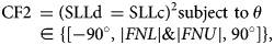
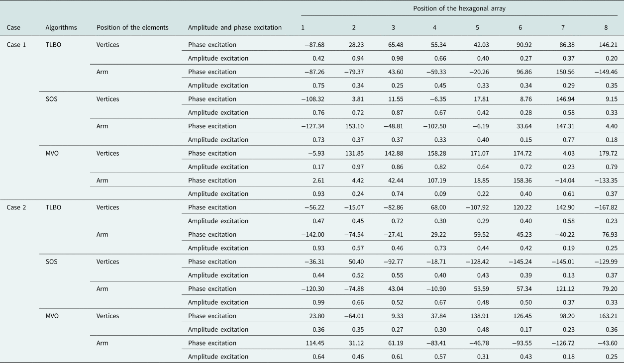
In Example 1, we have considered the eight-concentric hexagonal array of 3N (N = 6) isotropic antennas in each hexagon. The spacing between the elements of the first hexagonal array antenna is kept fixed at d_e = 0.5λ and the inter-ring spacing is d_h = 0.5λ. Four different cases are considered for other φ-planes. In Case 1, the optimization is carried out at the 0^o φ-plane and in Case 2, the optimization is performed at the 90^o φ-plane. The normalized synthesized power pattern together using all three algorithms is presented in Figs 5 and 6, for Case 1 and Case 2, respectively. The expected and calculated values of all the design variables are summarized in Table 1. Table 2 reports the phase excitation values corresponding to the flat-top beam using all three algorithms.

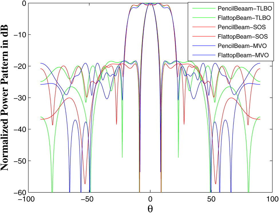
Fig. 5. Normalized power pattern in φ = 0^o plane for Example 1.

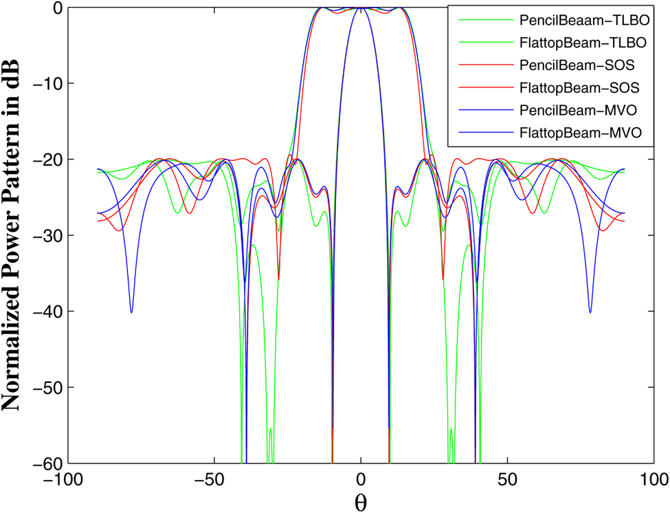
Fig. 6. Normalized power pattern in φ = 90^o plane for Example 1.

Table 1. Desired and obtained simulation values for Example 1.

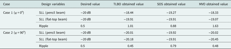
Table 2. Optimal set of radial phase excitation (in degrees) for flat-top beam and common normalized amplitude distribution for both the beams in Example 1.

Example 2 deals with the eight-concentric hexagonal array antennas of 2N (N = 6) isotropic antennas in each of the hexagon. The antennas are placed uniformly with a spacing d_e = 0.5λ in the first ring and the inter-ring spacing is kept at d_h = 0.5λ between two adjacent hexagonal arrays. The desired value for SLL for the pencil and flat-top beams is kept the same as the previous example, i.e. 20 dB for both the beams. Table 3 represents the expected and calculated values of the design variables for Example 2, using all three algorithms the two φ-planes. The global best value zero indicates that the obtained values of all the design parameters are lesser than the corresponding expected values. Table 4 gives the phase distribution of the elements present at the vertices and in the arms of each hexagon. The reconfigurable power patterns using TLBO, SOS, and MVO are presented together for 0^o and 90^o φ-planes in Figs 7 and 8, respectively.

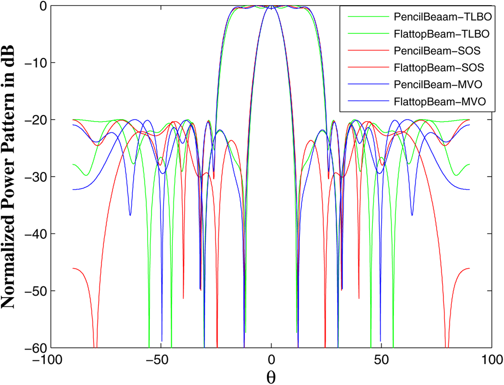
Fig. 7. Normalized power pattern in φ = 0^o plane for Example 2.

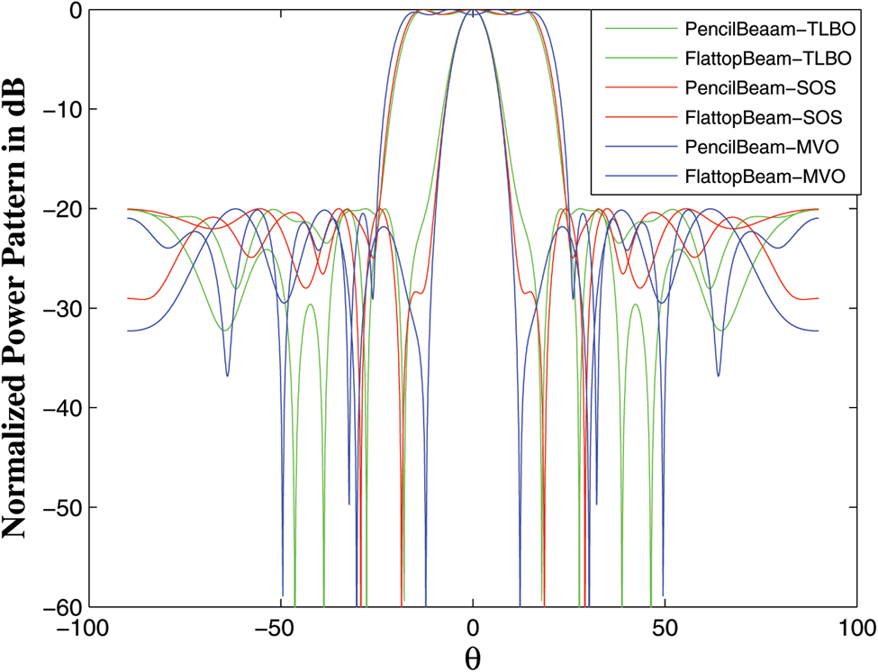
Fig. 8. Normalized power pattern in φ = 90^o plane for Example 2.

Table 3. Desired and obtained simulation values for Example 2.

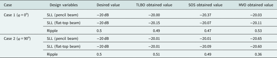
Table 4. Optimal set of radial phase excitation (in degrees) for flat-top beam and common normalized amplitude distribution for both the beams in Example 2.

It can be noticed that the inter-element spacing in each hexagon is sufficient enough to eliminate the effect of mutual coupling. All the algorithms prove their efficiency to reach the global solution of the optimization problem. From Tables 1 and 3, it can be noticed that the SOS algorithms perform better than the other two algorithms in terms of SLL and ripple for Case 1 in both examples. Whereas in Case 2 of Examples 1 and 2, MVO obtains improved SLL and ripple values compared to TLBO and SOS optimization algorithms. In general, both examples were able to produce reconfigurable beam patterns at two principle vertical planes. Though the structure considered in Example 2 can reach the desired values of all the design parameters with a lower number of array elements and smaller structures. Also, for Example 2, all three algorithms perform almost the same and able to achieve the design objectives. These three optimization algorithms do not have any tuning parameters; hence they can support stable results with minimal complexity. Also, the proposed optimization technique can produce reconfigurable beam patterns in different azimuth planes successfully with a negligible amount of ripple in the main beam of the flat-top pattern.