


I. INTRODUCTION
The experimental characterization of the low-frequency (LF) noise of microwave semiconductor devices under large-signal operation is a topic of active research these last years. An accurate description of the LF noise in compact models allows a more realistic optimization of circuits such as oscillators, in terms of phase and amplitude noise spectra performances.
The LF noise has often been considered to be function of only the DC current crossing the device. Under this assumption, the statistical properties of the LF noise are time invariant: the process is stationary.
The possibility of modulating a low-pass mechanism (the LF noise) with a high-frequency signal (the RF large-signal) has found some reluctancy, until simulation and experimental evidences started to come up, although not necessarily pointing to a general theory. The statistical properties of the LF noise would thus vary with the large signal: in the case of a periodic large signal, the process is cyclostationary.
In terms of the results predicted from physics-based simulations, one of the first studies on the field was carried out on a Monte-Carlo simulation of homogeneous semiconductor resistors [Reference Pérez, Gonzâlez, Delage and Obregon1], and evidenced the up-conversion of the trap-assisted generation-recombination (G-R)LF noise around the AC pump. Besides, Sanchez et al. [Reference Sanchez, Bosman and Law2] and Bonani et al. [Reference Bonani, Guerrieri and Ghione3] used drift-diffusion simulations on more realistic devices.
In the case of a linear resistor, such up-conversion is only possible if the microscopic white noise sources are first low-pass filtered and then HF modulated (a process known as filtering-modulation (FM) scheme [Reference Bonani, Guerrieri and Ghione3]). Interestingly, those simulation results support the experimental facts [Reference Lorteije and Hoppenbrouwers4] along with the empirical model of resistance fluctuations proposed two decades before.
In contrast, by first HF modulating and then low-pass filtering the microscopic noise sources (modulation-filtering (MF) scheme [Reference Bonani, Guerrieri and Ghione3]) the noise would be practically that of the stationary (DC) case: if the pump frequency is much higher than the corner frequency of the LF noise, no colored noise would be observable around the pump. This corresponds to the stationary concept.
The non-homogeneous case, such as in PN junctions, seems to be much less unanimous. Sanchez et al. use the FM scheme for diodes [Reference Sanchez, Bosman and Law2] and bipolar transistors [Reference Sanchez, Bosman and Law5], whereas Bonani et al. [Reference Bonani, Donati Guerrieri and Ghione6–Reference Bonani, Donati Guerrieri and Ghione9] stated that the MF scheme was somehow more adapted to the diode case.
To distinguish between the stationary and cyclostationary concepts, noise measurements under DC-only bias are not sufficient. This has been pushing model designers to create or to adapt existing setups with the goal of measuring LF noise while applying a periodic large signal to the device. Some examples of the setups used are given in the next section.
II. PREVIOUS EXPERIMENTAL INITIATIVES
The previous experimental initiatives over the behavior of LF noise under periodic excitation may be divided into two groups, depending on the pump frequency used.
A) LF pump
In this case, the pump frequency is of the order of the corner frequency of the LF noise being considered. This category comprises the pioneer work of Bull and Bozic [Reference Bull and Bozic10], on composition resistors, diodes and bipolar transistors, and the seminal paper by Lorteije and Hoppenbrouwers [Reference Lorteije and Hoppenbrouwers4] on the 1/f noise in carbon resistors.
To compare the frequency dependence of the excess noise near DC to that of the noise near the pump, Bull and Bozic used balanced circuits along with transformers to eliminate the AC signal at the input of the low-noise amplifier, and the frequency of the pump signal was 84 kHz [Reference Bull and Bozic10]. Instead of using transformers, Lorteije and Hoppenbrouwers used a high Common-Mode Rejection Ratio (CMRR) differential amplifier, and a pump signal between 200 Hz and 10 kHz [Reference Lorteije and Hoppenbrouwers4].
Sanchez and Bosman [Reference Sanchez and Bosman11, Reference Sanchez and Bosman12] used a setup inspired from [Reference Lorteije and Hoppenbrouwers4] to measure the voltage fluctuations at the base of bipolar transistors. They also employed bridge circuits and a differential amplifier, and pump frequencies of 650 Hz, 6.95 kHz, and 20 kHz. More recently, Lisboa de Souza et al. [Reference Lisboa de Souza, Nallatamby, Prigent and Obregon13] also used the ideas from [Reference Lorteije and Hoppenbrouwers4] to give an experimental evidence of the cyclostationary properties of 1/f noise sources of microwave varactors and transistors at the external ports. Details of that experimental setup will be given in Section V.
The use of a LF pump signal has some advantages: not only the instrumentation is generally more simple, but also the variables (current, voltage) of the device under test can be determined more accurately. As a drawback, in the case of microwave circuits it can be argued that such LF pump is well below the working frequency, and thus it is questionable whether the observations should hold with the RF large signal. As a matter of fact, noise generation is always associated with conductive elements which are frequency independent by definition (neglecting transit time effects). Moreover, it was experimentally shown that the results are insensitive to the pump frequency, even when the pump frequency is 50 times higher than the corner frequency of the LF noise [Reference Lisboa de Souza, Nallatamby, Prigent and Obregon13].
B) High-frequency pump
A high-frequency pump has been used to study the around-DC behavior of the current fluctuations at the base [Reference Gribaldo, Bary and Llopis14, Reference Borgarino, Florian, Traverso and Filicori15] and at the collector [Reference Borgarino, Florian, Traverso and Filicori15] of microwave bipolar transistors. Gribaldo et al. [Reference Gribaldo, Bary and Llopis14] and Borgarino et al. [Reference Borgarino, Florian, Traverso and Filicori15] used transimpedance amplifiers to directly measure the Power Spectral Density (PSD) of the current fluctuations, while pumping the transistor with several power levels of a signal at 3.5 GHz [Reference Gribaldo, Bary and Llopis14] or 4.4 GHz [Reference Borgarino, Florian, Traverso and Filicori15]. In those setups, the low and high frequency paths are separated with the aid of Bias Tees.
Rudolph et al. [Reference Rudolph, Lenk, Llopis and Heinrich16] measured the residual phase noise of a transistor operating as an amplifier near to linear operation, and compared the experimental data against the simulation results of three noise modeling approaches. The frequency of the injected signal was 3.5 GHz.
The advantage here is that we have practically the same working conditions of the final application, which is ideal in terms of characterization. However, a good level of accuracy of the non-linear parasitic capacitances of the device is necessary to validate the analysis, because their impact on the conversion processes is non-negligible.
Moreover, it will be shown that the experimental results of measuring directly the current fluctuations near DC (by means of transimpedance amplifiers) upon using a high-frequency pump are in line with our assumptions, but do not allow one to distinguish between a stationary or cyclostationary model.
III. A BRIEF NOTE ABOUT CONDUCTANCE FLUCTUATIONS
In this section, we review some concepts related to the model of conductance fluctuations, necessary to the understanding of the cyclostationary properties of the LF noise. We start with the noisy linear conductance shown in Fig. 1(a).

Fig. 1. Dynamic noisy conductance (a) represented, at an angular frequency Ωn, by a pseudo-sinusoidal conductance term (b). In (c), a possible implementation using a current-noise source.
The noise of the conductance at an angular frequency Ωn is expressed by a pseudo-sinusoidal (fluctuating) conductance term in parallel to the deterministic (mean) conductance (see Fig. 1(b)).
If the noisy conductor is driven by a deterministic constant (DC) voltage, say v(t) = V 0, it is straightforward to see that there will be a sinusoidal current fluctuation at angular frequency Ωn given by i n = V 0g n cos(Ωnt + Φn).
If now the device is driven by a deterministic sinusoidal voltage at angular frequency ωp, say v(t) = V p cos(ωp × t), there will be a current fluctuation at angular frequencies ωp ± Ωn given by i n = (V pg n/2) cos ((ωp ± Ωn) × t + Φn) and no current fluctuation at angular frequency Ωn. Because the system is linear, the superposition theorem holds, that is, if the driving signal is comprised of both DC and AC components, excess noise will be observed around DC as well as around the pump. More importantly, the noise components at angular frequencies Ωn and ωp ± Ωn will be completely correlated. The behavior described above has been experimentally observed, for example, in carbon resistors [Reference Lorteije and Hoppenbrouwers4, Reference Jones and Francis17].
So the current fluctuation is proportional to the instantaneous deterministic current crossing the device. To arrive at the model shown in Fig. 1(c), we note that the voltage applied is related to the deterministic current crossing the device by means of the deterministic conductance g d, that is, v(t) = i(t)g d−1. In a first-order approximation, the same conclusions can be found by considering a series resistance arrangement, as in the model of resistance fluctuations proposed by Lorteije and Hoppenbrouwers [Reference Lorteije and Hoppenbrouwers4] to explain their experimental observations.
Since the noise current variation in ![]() is proportional to the instantaneous current crossing the device, the current-noise PSD in units of A2/Hz is proportional to the square of the instantaneous current (i(t)). If we further introduce a 1/f-like frequency dependency in the coefficient g n, we arrive at the following equation:
is proportional to the instantaneous current crossing the device, the current-noise PSD in units of A2/Hz is proportional to the square of the instantaneous current (i(t)). If we further introduce a 1/f-like frequency dependency in the coefficient g n, we arrive at the following equation:
where CF stands for conductance fluctuations. The PSD is function of frequency and time, and has units of A2/Hz. Such a PSD (time-dependent) is generally referred to as the instantaneous Spectral Density [Reference Gardner18]. Equation (1) explicitly shows the amplitude-modulation of the noise source by the instantaneous value of the current crossing the device.
The relation above has been verified experimentally for a number of different carbon resistance specimens and authors (including the present authors). The discussion over the experimental observation of noise near DC under AC-only bias [Reference May and Sellars19], which is not explained by the conductance fluctuations model above and is generally attributed to non-linearities of the sample, is out of the scope of this paper. The dependence in equation (1) has been empirically adopted to model the noise in bipolar transistors with cyclostationary sources to simulate phase noise in MMIC oscillators [Reference Nallatamby, Prigent, Camiade, Sion, Gourdon and Obregon20].
Equation (1) states that the current-noise process may be non-stationary. In the case of a periodic (time-variant) deterministic current, the autocorrelation function as well as the PSD of the current noise will be periodic in time: the process is cyclostationary. By contrast, if we had assumed the noise to be dependent only on the (time-invariant) DC current crossing the device I 0, we would arrive at the widely known PSD expression
for which the noise process is modeled as stationary. The PSD is only function of frequency and has units of A2/Hz.
We emphasize that, for both cyclostationary and stationary concepts (equations (1) and (2), respectively), the PSD of the current noise around DC is only dependent on (the square of) the mean (DC) component of the deterministic current crossing the device. That is why noise measurements under DC-only bias are not sufficient to distinguish between those two concepts.
What is more subtle is that when pumping the element by a periodic deterministic signal, the current noise observed around DC should be unaffected as far as the DC deterministic current is kept constant, which has been experimentally observed through the use of transimpedance amplifiers [Reference Gribaldo, Bary and Llopis14, Reference Borgarino, Florian, Traverso and Filicori15]. One may erroneously conclude that the LF noise is not affected by the pump signal, and it should thus be a stationary process.
In this context, the striking difference between the stationary and cyclostationary concepts is illustrated in Fig. 2, in which the noisy conductance is being driven by a periodic signal.

One can see that in the case of a cyclostationary process (equation (1)), the current noise around the pump frequency can be as high as that around DC, even if the pump frequency is much higher than the corner frequency of the LF noise. This is not the case for a stationary process.
As a conclusion, in the case of linear resistors made up of carbon, the FM scheme (represented here by the model of conductance fluctuations) is in close agreement with experimental results. Of utmost importance is the fact that excess noise is observed around the pump frequency in a linear system. Thus, the conversion of LF noise to around-carrier noise (such as phase noise in oscillators) is not exclusively due to the non-linear properties of the active device, but also due to the intrinsic cyclostationary properties of noise sources.
IV. CIRCUIT UNDER INVESTIGATION
Having used the analysis of the LF noise of a linear resistor to improve comprehension, we move forward to the more interesting case of a non-linear device. In our case, the circuit under consideration is a bipolar junction, which can be a diode or the base-emitter junction of a bipolar transistor. For simplicity, the diode case is shown in Fig. 3(a).

Fig. 3. Circuit under investigation (a), current–voltage relation of the diode (b) and equivalent model for large-signal small-signal analysis (c). In (a), RS primarily represents an external high-value wire-wound resistor (see Fig. 6), but it also includes the minor effects of the access resistance of the diode and the internal resistance of the DC and AC signal sources.
The current-noise source, the properties of which we want to determine, is placed in parallel to the convective deterministic element. The use of a current source to represent 1/f noise is deliberate: thermal effects may greatly impact the input impedance of bipolar transistors, depending upon collector biasing conditions. For each collector biasing condition, a different frequency-dependent input impedance and corresponding frequency-dependent voltage noise PSD are found. However, under generally observed conditions, when dividing the latter by the square of the former the same current-noise PSD curve is obtained, regardless of collector biasing conditions [Reference Lisboa de Souza, Nallatamby, Prigent and Obregon21]. So the current-noise source better represents the physical origins of noise, the voltage noise being the consequence of the product of the current noise by the impedance of the device.
The noiseless junction is characterized by a voltage–current (Fig. 3) relation defined in the time domain as
for which I S is the diode saturation current, η is the diode ideality factor, and V th is the thermal voltage (25.9 mV at 300 K).
The diode is supposed to work in large-signal operation. Thus, its instantaneous current can be described as (f p represents the pump frequency)
By taking the derivative of equation (3) with respect to the voltage applied, we arrive at the well-known linear periodically time-varying equivalent conductance of the diode:
The inverse of the instantaneous conductance is the instantaneous equivalent resistance of the diode:
Interestingly, the instantaneous small–signal resistance of the diode (equation (6)) is inversely proportional to the instantaneous (deterministic) diode current. We recall that in the model of conductance fluctuations, the current noise (in ![]() ) is proportional to the deterministic current.
) is proportional to the deterministic current.
Please note that, as pointed out in [Reference Maas22], I d(t) and V d(t) do not need to be time invariant (DC): the only restriction in equations (5) and (6) is that the signals for which the conductance is computed (i d(t), v d(t)) be much smaller that the large signal (I d(t)). This is certainly the case of noise. Moreover, there is no restriction on the frequency relation between small and large signals.
Since the time-varying resistance of the diode is in parallel to the series resistance (see Fig. 3(c)), the equivalent resistance seen by the current source is given by

for which
In the above equations, f p and T p represent the pump frequency and period, respectively. Equation (7) remains valid even for the static case, for which only R eq0 is non-zero and given by
This value is often used in the static case to compute the equivalent short-circuit current-noise source from the voltage noise measured [Reference Lisboa de Souza, Nallatamby and Prigent23].
If we consider a time-variant biasing, let us take a look at what happens to the spectral components of the resistance seen by the current noise (equation (8)) when we increase V AC while adjusting V DC to keep I 0 unchanged. This is illustrated in Fig. 4, for which I S = 4.5 × 10⁻¹⁸A, η = 1.06, R S = 2000 Ω, and I 0 = 100 µA.

Fig. 4. Spectral components of R eq(t) as a function of the ratio of I 1 and I 0.
The process of converting current noise (whether stationary or cyclostationary) in parallel to a time-varying circuit into voltage noise is based on the small-signal large-signal analysis (also known as parametric analysis) inspired from the mixer theory [Reference Saleh24]. It comprises a convolution between current and resistance spectral terms and is illustrated in Fig. 5. It relates voltage and current spectral components at frequencies nf p ± f n, where f n is the noise frequency while f p is the fundamental frequency of the large signal.
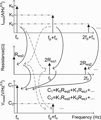
Fig. 5. V noise computation as a spectral convolution of current and resistance. For simplicity, not all frequency components are shown. Please consider f x = 1 Hz throughout the text. The term 2 “disappears” in the value of C 1, C 2, … since the product of two cosines (impedance and current noise) gives a term multiplied by 0.5.
From our analysis so far, we may envisage two different scenarios. If the current noise is a stationary process, that is, if the noise should be described by equation (2), the PSD of the voltage noise around DC measured across the diode should increase with pumping. This is a direct consequence of the fact that the noise around the pump frequency is negligible (see Fig. 2(c)). In this case, the voltage noise around DC is approximately given by product of K 0 and R eq0K 0 is independent of the pumping level, because the current I 0 is kept fixed. However, R eq0 increases with the pumping level (see Fig. 4), and so the voltage noise.
If we now consider a cyclostationary process, SInoise around the pump frequency can be as much as (and is correlated with) that around DC. This, along with the fact that R eq1 is negative and whose module can approach R eq0, will decrease S V noise around DC as I 1 increases (as I 1 increases, other current components are created, and the analysis should be extended to R eq2, R eq3, …. A complete analysis still points to a monotonic decrease of S V noise though) [Reference Lisboa de Souza, Nallatamby, Prigent and Obregon13].
What is interesting is to see what happens to a current driven diode (R S = ∞) in Fig. 3(c)) whose current-noise PSD follows equation (1). Since the current noise (in ![]() ) varies as the deterministic current and the diode instantaneous resistance varies as the inverse of the deterministic current, their time-domain product generates a stationary voltage noise (there will not be voltage sidebands around the pump). Obviously, the same result is obtained from harmonic balance simulations.
) varies as the deterministic current and the diode instantaneous resistance varies as the inverse of the deterministic current, their time-domain product generates a stationary voltage noise (there will not be voltage sidebands around the pump). Obviously, the same result is obtained from harmonic balance simulations.
Those two different scenarios will be checked against experiments.
V. EXPERIMENTS
Following the ideas proposed in [Reference Lisboa de Souza, Nallatamby, Prigent and Obregon25], to collect the experimental data we will use the setup shown in Fig. 6, which is much based on the original work of Lorteije and Hoppenbrouwers [Reference Lorteije and Hoppenbrouwers4]. It is composed of a high-purity LF source (including DC offset) internal to the vector signal analyzer Agilent 89410A, and a low-noise differential amplifier connected to the devices under test (DUTs). The DUTs are disposed in a bridge configuration, and biased through large series wire-wound resistors.

Fig. 6. Setup used in our measurements.
The setup is used for measuring the PSD of the voltage fluctuations across the arms of the bridge, under both static and large-signal operations. In this work, we will focus our analysis on the experimental data collected from the SiGe microwave transistor BFP740F, manufactured by Infineon Technologies. Similar conclusions were drawn for other transistors and diodes [Reference Lisboa de Souza, Nallatamby, Prigent and Obregon13]. In our simulations, we used the following values: I S = 4.5 × 10⁻¹⁸ A, η = 1.06, and R S = 2000 Ω (see Fig. 3).
A) Static operation
Initially, the DC level of the source (V DC) is adjusted as to vary I 0 in each arm, while the AC component is switched off (−120 dBm). For each value of I 0, an impedance probe (HP4194A) is connected to one of the DUTs, and the impedance seen by the equivalent current-noise source of the DUT (in this case given by equation (9)) is measured. The measured impedance will be used to convert the voltage noise PSD to be measured into a current-noise PSD [Reference Lisboa de Souza, Nallatamby and Prigent23].
The amplifier is then connected, and the PSD of the voltage fluctuations across the two arms are measured for each value of I 0. Moreover, the noise is compared to that measured with just one branch (second amplifier input being grounded) while the circuit is biased with a filtered lead-acid battery (circuit not shown). For each value of I 0, the voltage noise power measured from the bridge is approximately twice that measured with just one branch, as expected. This means that not only the noise from the internal source is being properly cancelled out due to the balanced bridge, but moreover the DUTs can be considered stochastically uncorrelated.
Even if we measure the voltage noise PSD across the arms of the bridge, we will present the equivalent curves for each arm. The dependence of the voltage and current-noise PSDs with I 0 is shown in Fig. 7.

Fig. 7. Dependence of the voltage and current-noise PSDs with I 0. The frequency of analysis is 100 Hz.
The fact that the voltage noise PSDs are roughly independent of I 0 comes from the high value of R S (thus r dc is practically given by the impedance of the DUT) along with the I 02 dependence of the current-noise PSD, as seen in the bottom of the figure. Since the current-noise PSD is proportional to the square of the static current, and the square of the time-invariant resistance is proportional to the inverse of the square of the current, their product (the voltage noise PSD) is invariant.
B) Large-signal operation
During large-signal operation, we control the bias as to keep the DC current (I 0) fixed. In our case, we adopted I 0 = 100 µA. The pump frequency is 100 kHz, implying that the circuit may be considered to be purely resistive up to the frequency at which the reactive parts of the wire wound resistors and the DUT itself start to show up, which is well above the 10th harmonic of the pump frequency.
The first step consists of removing the low-noise amplifier, and to connect the second channel (high input impedance) of the analyzer directly onto one of DUTs. With a straightforward manipulation on the voltage measured at channels 1 and 2, and knowing the approximate value (to within 1%) of R S, it is possible to determine the instantaneous current crossing the branches. This way, we determine the source levels (including both DC and/or AC amplitudes) necessary to set the current spectral components as desired.
Similar to the static case, the DC and AC levels of the source are adjusted as to vary I 1, while keeping I 0 fixed. The spectral components of the current as well as the time-domain waveforms of the current and voltage across the device are measured, and compared to the simulation results, as a mean to validate our purely resistive model and to ensure the device is working within allowed limits. Such comparison is illustrated in Fig. 8, which shows an excellent agreement between measurement and simulation, as expected.

Fig. 8. Comparison between measured and simulated waveforms (voltage and current).
Then, for each value of I 1 an impedance probe (HP4194A) is connected to one of the DUTs, and the DC component of the impedance seen by the equivalent current-noise source of the DUT (in this case given by equation (8) with n = 0, see R eq0 in Fig. 4) is measured. A more elaborate technique would enable the measurement of higher spectral components of R eq(t) (R eq1, R eq2, …). Figure 9 presents a comparison between measured and simulated values for three values of I 1. As can be seen, a good agreement is found.

Fig. 9. Comparison between measured and simulated values of R eq0.
The amplifier is then connected to the bridge, and the series resistances are adjusted (to within 1%) as to maximize the attenuation from channel 1 to channel 2, that is, the capacity of the system bridge + amplifier to balance the pump out. In general, the same adjustment gives good results for all the biasing points to be used. The attenuation, which is function of the large-signal bias point and pump frequency, is used to compute the noise from the signal source induced into the bridge. Thus, if for a given configuration the attenuation from channel 1 to channel 2 is 40 dB, the noise power (in V2/Hz) measured at channel 1 is reduced by 40 dB and plotted against the noise measured at channel 2. For all measurements performed, the noise power induced was at least 20 dB below the noise power measured at channel 2.
Figure 10 presents the dependency of the around-DC and around-carrier behavior of S V noise with I 1. It includes a comparison between the measured values and those obtained from simulations by implementing either equation (1) or (2).

Fig. 10. Dependency of the around-DC and around-carrier behavior of S V noise.
It can be seen that for high pumping levels, there is a difference of up to 20 dB between the voltage noise computed by implementing equation (1) or (2). Such difference eliminates any possibility of doubt on whether a stationary or cyclostationary description of the LF noise should be used in the LF noise compact model of the device analyzed. The model of conductance fluctuations (equation (1)) is certainly the most adequate to represent the LF noise of such device. Moreover, it is interesting to note the non-monotonicity of the PSD of the voltage noise around the pump.
C) Discussion
The preceeding section presented an evidence of a semicondutor device whose LF noise manifests as conductance fluctuations. Under static biasing, its S I noise showed a I 02 dependence. Under large-signal operation, it was brought to light that actually equation (1) should be used to describe its LF noise.
This conclusion is, however, far from being universal. Under static biasing, semiconductor devices may show a dependence of S I noise on I 0k, with k typically varying between 1 and 3. In this case, a more flexible approach should be used: the PSD of the current-noise sources should be partially dependent on the DC component of the deterministic current and partially on the instantaneous current [Reference Nallatamby, Prigent, Camiade, Sion, Gourdon and Obregon20]. A specific dependence on each individual spectral component of the current could be also envisaged.
The characterization method shown here, based on the measurement of the voltage fluctuations around DC and around carrier, is currently being used to address such cases.
We must emphasize that measuring the voltage fluctuations across the device is much more interesting than measuring directly the current fluctuations around DC by using transimpedance amplifiers: the former allows a difference of up to 20 dB between the stationary or cyclostationary concepts, whereas the latter would give no difference. We thus believe that the measurement technique presented here is the most precise for characterizing the cyclostationarity coefficients of LF noise.
VI. CONCLUSION
We presented a detailed analysis, simulation results, and experimental data concerning the LF noise of microwave bipolar devices operated under large-signal regime.
It was shown that the LF noise is indeed a cyclostationary process, being (at least partially) dependent on the instantaneous current crossing the device. The LF noise is thus a parametric variation of the conductance of the device.
We propose a characterization method that, we believe, is the most reliable method in terms of accuracy to determine the cyclostationary coefficients of the equivalent current-noise sources.
 Antonio Augusto Lisboa de Souza received the B.Sc and M.Sc degrees in Electronics from Federal University of Campina Grande (Brazil) in 1998 and 2001, respectively, and the Ph.D. degree in Electronics from the University of Limoges (France) in 2008. His research interests concern compact modeling of microwave active devices, with a special emphasis on low-frequency noise characterization and modeling of HBTs.
 Emmanuel Dupouy received the Master's degree in Sciences et Technologies de l'Information et de la Communication from the University of Nice-Sophia-Antipolis, France, in 2005. He is currently working toward the Ph.D. degree at the XLIM Research Institute, University of Limoges. His research interests concern phase noise reduction in oscillators.
 Jean-Christophe Nallatamby received the DEA degree in microwave and optical communications in 1988, and the Ph.D. degree in Electronics from the University of Limoges, France, in 1992. He is now lecturer in GEII Department at Brive of the IUT at the University of Limoges. His research interests are non-linear noise analysis of non-linear microwave circuits, the design of the low phase noise oscillator and the noise characterization of microwave devices.
 Michel Prigent received the Ph.D. degree from the University of Limoges, France, in 1987. He is Professor at the University of Limoges. His field of interest is the design of microwave and millimeter wave oscillator circuits. He is also involved in characterization and modeling of non-linear active components (FET, PHEMT, HBT, etc.) with a particular emphasis on low-frequency noise measurement and modeling for the use in MMIC CAD.
 Juan Obregon received the E.E. degree from CNAM, Paris, France, in 1967 and the Ph.D. degree from the University of Limoges, France, in 1980. He joined the Radar Division of Thomson-CSF, where he contributed to the development of parametric amplifiers for radar front ends. He then worked at RTC Laboratories, performing experimental and theoretical research on Gunn oscillators. He joined the DMH Division of Thomson-CSF in 1970 and became Research Team Manager. He was appointed as Professor at the University of Limoges in 1981. His fields of interest are the modeling, analysis, and optimization of non-linear microwave circuits, including noise analysis. Since 1981 he has been a consultant to microwave industrial laboratories. He is now Professor emeritus at the University of Limoges.


