


Introduction
Passive intermodulation (PIM) distortion, which is induced by the nonlinear characteristic of passive components, is regarded as a serious problem in microwave communication systems [Reference Wilkerson, Kilgore, Gard and Steer1, Reference Zhao, He, Ye, Gao, Peng, Li, Bai and Cui2]. The nonlinear effect limits the capacity of the communication systems. Thus, it becomes one of the main limiting factors of developing highly linear systems.
The contact nonlinearity of passive microwave devices is generally more serious than material nonlinearity in microwave communication systems. And it is caused by the nonlinear effects, such as the electron tunneling effect, the thermionic emission, micro-discharge, and electrostriction [Reference Lui and Rawlins3–Reference Li, Zhang, Jiang and Ma5]. Yang [Reference Yang, Wu, Xu, Zhang, Stutts and Pommerenke6] presented a measurement system based on the acoustic vibration to locate PIM sources in the base station antennas. Mantovani et al. [Reference Mantovani and Denny7, Reference Mantovani, Denny and Warren8] proposed a method for locating PIM sources in an environment of many metal-metal junctions, which utilized two-tone signal to generate PIM products in the metal-metal junction that was subjected to an acoustic wave. The mechanical vibration causes PIM products to become amplitude modulated at the frequency of the acoustic illumination. Henrie and Christianson [Reference Henrie, Christianson and Chappell9–Reference Henrie, Christianson and Chappell11] built the theoretical PIM model for microwave coaxial connectors and conducted a large number of experiments to verify the results. Wetherington and Steer [Reference Wetherington and Steer12] studied PIM effect in a log-periodic dipole array antenna with standoff acoustic excitation, which is due to acousto-electromagnetic coupling. Kilgore et al. [Reference Kilgore, Kabiri, Kane and Steer13] studied the effect of chaotic vibrations on co-site interference and monopole antenna characteristics and measured the additional spectral content of antenna under vibration.
For the microwave connector, there are seldom literatures to describe the effect of surface roughness and vibration on PIM. Chen et al. [Reference Chen, He, Yang, Cui, Zhang, Pommerenke and Fan14] studied the passive intermodulation behavior on the coaxial connector and proposed a contact model of a contact unit. Yang et al. [Reference Yang, Wen, Qi and Fan15] presented an equivalent circuit model to analyze PIM of loose contact coaxial connectors. They studied the contact behavior of microwave connectors from the macroscopic perspective. However, the microscopic contact behavior of connectors is still unknown. Greenwood and Williamson (GW) constructed an elastic contact model, which described the deformation depending on the surface topography. The GW model assumes that all asperity summits have the same radius and a Gaussian distribution of asperity heights and uniform distribution of asperities over the projected in-plane surface area. However, the GW model cannot completely describe the rough surface profile, such as asperity shape and size information. With the improvement of the measurement precision of rough surface, the microscopic morphology of rough surface is revealed and presents fractional characteristics. Weierstrass–Mandelbrot (WM) model can solve this problem only depending on the fractional parameters of surface roughness [Reference Mandelbrot16]. Majumdar and Bhushan [Reference Majumdar and Bhushan17] studied the elastic-plastic contact between one-dimensional rough surfaces based on the fractional theory and used a power-law relation for the fractional size-distribution of contact spots. Fu et al. [Reference Fu, Choe, Jackson, Flowers, Bozack, Zhong and Kim18] conducted a lot of experiments for vibration–induced wear of silver-plated high power connectors. They showed that the change of electrical contact resistance of the connector during vibration mainly owed to the changed contact area. Zhang and Flowers [Reference Zhang and Flowers19] investigated the fact that the major reason of connector failure was the vibration-induced wear corrosion. In the practical working environment of connectors, the vibration is a common working condition. However, there is no research to reveal the effects of vibration on PIM of microwave connectors. Generally, the vibration load may affect the microscopic contact of connectors which has an impact on PIM of connectors.
In this paper, an experimental investigation is performed to quantify PIM which is influenced by the contact stress and contact surface roughness during vibration. Meanwhile, the relations among the PIM power level and torque applied on the connector, acceleration, and duration are revealed. The analysis and simulation methods are shown for understanding the PIM generation. The paper is organized as follows. In the section “Principles”, the WM model and PIM point source model are introduced. Then, a power spectral density method based on surface roughness is presented to identify the roughness parameter of the contact surface. In the section “Measurements”, in order to reveal the behavior of PIM during vibration, several experiments are implemented. The finite element model of the connector is built in ANSYS software, and the simulations with different loads are performed. We import the stress from the simulation into the PIM point source model and get the calculation results which are verified by experimental results. In the section “Conclusions”, the conclusions are summarized.
Principles
The WM model is adopted for describing the rough surface and given as [Reference Ausloos and Berman20]:
 $$\eqalign{z\left( {x,y} \right) & = L(G/L)^{(D-2)}\left( {\displaystyle{{\ln \gamma } \over M}} \right)^{1/2}\sum\limits_{m = 1}^M {\sum\limits_{-n_{\max }}^{n_{\max }} {\gamma ^{\left( {D-3} \right)n}} } \cr & \quad \times \left\{ {\cos \phi _{m,n}-\cos [k_{\rm 0}\gamma ^n{(x^2 + y^2)}^{1/2}} \right. \cr & \quad \times \left. {\cos ({\tan }^{-1}\left( {y/x} \right)-{{\theta }^{\prime}}_m) + \phi _{m,n}]} \right\},} $$
where z(x, y) is the height of rough surface in Cartesian coordinates (x, y). L is the sample length, k 0 is a wave number related to L, and k 0 = 2π/L. M is the number of unidirectional corrugation layers which contributes to the WM model. D is the fractional dimension, while G is the roughness parameter. γ is the base of the frequency and γ>1.  ${\theta} ^{\prime}_m$ determines the direction of the stacked layers of corrugation, we make
  ${\theta} ^{\prime}_m = \pi m/M$ to get uniform distribution. ϕ m,n is a set of independent random phase, which is evenly distributed in the range of [0, 2π].
According to the WM model, the surface roughness is obtained via two roughness parameters: fractional parameter D and roughness parameter G.
The vibration is the external load applied to the connector. The effect of vibration on PIM is mainly manifested in the change of contact force and actual contact area which can be obtained by ANSYS software. And the change of surface contour after vibration can be measured by surface roughness meter. The contour is used to construct the actual surface model based on the WM model.
Based on the WM model and surface information, a FEM model of the rough surface can be established. In the ANSYS software, the actual contact area for different loads can be obtained, which is used to calculate the parameters of the equivalent circuit shown in Fig. 1. Constriction resistance R t results from current constriction effect, and contact resistance R const represents the electrical characteristics of metal-metal contact. Tunneling resistance R tv results from tunneling effect, and contact capacitance C c represents the electrical characteristics of the metal-insulator-metal structure. Non-contact capacitance C nc and non-contact resistance R ninc are electrical parameters of non-contact areas.

Fig. 1. The equivalent circuit model.
The constriction resistance R t can be calculated as [Reference Li, Zhai, Li, Ma and Jiang21]:
 $$R_t = f_1(\lambda /r_a)\displaystyle{\rho \over {2r_a}} + \displaystyle{{4\rho \lambda} \over {3A_r}},$$
where f 1(λ/r a) = (1 + 0.83(λ/r a))/(1 + 1.33(λ/r a)) is interpolation function. λ is electron free path for the contact material, ρ is contact metal resistivity, r a is the average radius of the asperity contact circle, and A r is actual area of contact.
The metal contact resistance R const can be calculated as:
 $$R_{const} = \displaystyle{\rho \over {2r_{MM}N_c}}f_2\left( {\displaystyle{{r_{MM}} \over {r_a}}} \right),$$
where r MM is the equivalent MIM contact radius of a single asperity and N c is the number of micro-asperities, the expression of  $f_2(r_{MM}/\bar{r}_a)$ is as follows:
 $$\eqalign{& f_2\left( {\displaystyle{{r_{MM}} \over {{\bar{r}}_a}}} \right) = 1-1.41581\left( {\displaystyle{{r_{MM}} \over {{\bar{r}}_a}}} \right) + 0.06322\left( {\displaystyle{{r_{MM}} \over {{\bar{r}}_a}}} \right)^2 \cr & \quad\qquad\qquad + 0.15261\left( {\displaystyle{{r_{MM}} \over {{\bar{r}}_a}}} \right)^3 + \;0.19998\left( {\displaystyle{{r_{MM}} \over {{\bar{r}}_a}}} \right)^4,} $$
in which,  $\bar{r}_a$ is the mean value of r a.
The tunnel resistance R tv is based on tunnel current. It can be calculated as:
 $$\eqalign{R_{tv} = &\displaystyle{V \over {A_SJ_{tv}}} \cr J_{tv} = &\displaystyle{e \over {2\pi hs^2}}\left( {\varphi_0e^{-4\pi \sqrt {\displaystyle{{2m\varphi_0} \over {h^2}}} s}-(\varphi_0 + eV)e^{-4\pi \sqrt {\displaystyle{{2m(\varphi_0 + eV)} \over {h^2}}} s}} \right),} $$
where, J tv is the tunnel current density, A S is the tunnel area, φ 0 is the work function of metal, s is the thickness of barrier in the Fermi level, h is the Planck constant, m is the mass of electron. The tunnel current is the dominant nonlinear source in MM contact [Reference Zhang, Li and Jiang22].
The contact capacitance is C c = ε rε 0A nA*/s, where ε r is the relative dielectric permittivity of the insulating film on the metal, ε 0 is the vacuum dielectric permittivity, A n is the nominal contact area and A* is the dimensionless ratio of real contact area and nominal contact area. The non-contact resistance R ninc is considered infinite in practice. The non-contact capacitance is C nc = ε 0(A n − A r)/d, where d is the distance between the up and down non-contact area.
In microwave connectors, PIM is related to the nonlinear I–V relationship of contact area. Thus, we can derive the PIM power level by the nonlinear I–V characteristic. A polynomial model is used to describe the nonlinear I–V relationship [Reference Li, Zhang and Jiang23].
 $$I = \sum\limits_{i = 1}^\infty {C_iV^i}, $$
where the input voltage V can be obtained from the input power of the connector. The nonlinear I–V relationship which derives from Fig. 1 is as follows:
 $$\left\{ {\matrix{ {I = \displaystyle{{V-V_c} \over {R_t}} + C_{nc}\displaystyle{{dV} \over {dt}}{\rm}} \cr {V = \left( {C_c\displaystyle{{dV_c} \over {dt}} + \displaystyle{{V_c} \over {R_{const}}} + \displaystyle{{V_c} \over {R_{tv}}}} \right)R_t + V_c} \cr}} \right.,$$
where I is the total current through contact node. V is the voltage at the two ends of the circuit, and V c is the voltage across the C c. After discretization, the numerical solution of equation (7), which is used to construct the nonlinearity I–V curve, is obtained by Euler method. Then the numerical solution is used to calculate the parameters C i in equation (6) which is a linear equation group.
In communication systems, the third-order PIM product is most likely to fall into the receive band, the prediction of third-order PIM power level is important in PIM analysis. In the two-tone test, we defined
 $$V(t) = V_1\sin (\omega _1t) + V_2\sin (\omega _2t),$$
Based on the mathematical analysis, the current of the third-order intermodulation product I PIM3, which contributes to the third-order PIM power level, is as follows:
 $$\eqalign{I_{PIM3} &= \displaystyle{3 \over 4}C_3V_1^2 V_2 + \displaystyle{5 \over 4}C_5V_1^4 V_2 + \displaystyle{{15} \over 8}C_5V_1^2 V_2^3 \cr & \quad + \displaystyle{{105} \over {64}} C_7V_1^6 V_2 + \displaystyle{{105} \over {16}}C_7V_1^4 V_2^3 \cr & \quad+\displaystyle{{105} \over {32}}C_7V_1^2 V_2^5 + \cdots,} $$
Finally, the third-order PIM power level is derived by:
 $$P_{IM3} = \displaystyle{1 \over 2}Z_0\vert {I_{PIM3}} \vert ^2,$$
where Z 0 is the impedance of the DIN 7/16 connector, which is 50 Ω.
Based on the WM model, the fractional dimension D of actual contact surface must be obtained for the model construction of the connector. The rough surface contour of device under test (DUT) is measured by surface roughness meter. And the power spectral density method is used to identify the fractional dimension D.
For actual microwave connectors, the power spectral density method is a vital process to identify roughness parameter, which is used to calculate contact stress. According to equation (1), the one-dimension WM model can be written as:
 $$\eqalign{z(x) & = L\left( {\displaystyle{G \over L}} \right)^{D-1}(\ln \gamma )^{1/2} \cr & \times \sum\limits_{n = 0}^{n_{\max}} {\displaystyle{{\lsqb {\cos \phi_n-\cos \lpar {2\pi \gamma^nx/L + \phi_n} \rpar } \rsqb } \over {\gamma ^{\lpar {2-D} \rpar n}}}}}, $$
And its complex form is:
 $$\eqalign{z(x) = &\;L\left( {\displaystyle{G \over L}} \right)^{D-1} \cr& \times (\ln \gamma )^{1/2}\sum\limits_{n = 0}^{n_{\max}} {\displaystyle{\matrix{\lpar {\cos \phi_n + j\sin \phi_n} \rpar -\lsqb {\cos \lpar {2\pi \gamma^nx/L + \phi_n} \rpar } \hfill \cr {\quad + j\sin \lpar {2\pi \gamma^nx/L + \phi_n} \rpar } \rsqb \hfill} \over {\gamma ^{\lpar {2-D} \rpar n}}}} \cr {\rm} = &\;L\left( {\displaystyle{G \over L}} \right)^{D-1}(\ln \gamma )^{1/2}\sum\limits_{n = 0}^{n_{\max}} {\displaystyle{{\lpar {1-e^{\,j2\pi \gamma^nx/L}} \rpar e^{\,j\phi _n}} \over {\gamma ^{\lpar {2-D} \rpar n}}}},} $$
Introducing the impulse function δ(*), then the Fourier transform of z(x) is:
 $$\eqalign{& WM_{FT}(k) = FT\lsqb {z(x)} \rsqb = L\left( {\displaystyle{G \over L}} \right)^{D-1}(\ln \gamma )^{1/2}\sum\limits_{n = 0}^{n_{\max}} {\displaystyle{{\exp \lpar {\,j\phi_n} \rpar } \over {\gamma ^{\lpar {2-D} \rpar n}}}} \cr & \quad\quad\quad\quad\quad \times \lsqb {2\pi \delta \lpar k \rpar -2\pi \delta \lpar {k-2\pi \gamma^n/L} \rpar } \rsqb}, $$
where k is the spatial frequency.
Ignoring the term of zero frequency, it follows that:
 $$WM_{FT}WM_{FT}^{^\ast} = 4\pi ^2L^{4-2D}G^{2D-2}\ln \gamma \left[ {\sum\limits_{n = 0}^{n_{\max}} {\displaystyle{{\delta^2\lpar {k-2\pi \gamma^n/L} \rpar } \over {\gamma^{2n\lpar {2-D} \rpar }}}}} \right],$$
The power spectral density function is defined as:
 $$S(k) = \mathop {\lim} \limits_{T\to \infty} \displaystyle{{WM_{FT}WM_{FT}^{^\ast}} \over {2\pi T}},$$
where T is the integral interval of Fourier transform. Thus the property of S(k) is as follows:
 $$S(k)\propto \sum\limits_{n = 0}^{n_{\max}} {\displaystyle{{\delta ^2\lpar {k-2\pi \gamma^n/L} \rpar } \over {\gamma ^{\lpar {4-2D} \rpar n}}}}, $$
We can extract the peak values from the double logarithmic of power spectral density and fit a straight line, the fractional roughness D will be calculated from the slope of the straight line.
 $$D = \lpar {slope + 6} \rpar /2,$$
From the physical meaning of G, we define G = Ra, Ra is the roughness parameter, which is the arithmetical mean deviation of the assessed profile. So far, the method of parameters identification is presented. The WM model of actual contact surface can be constructed and the equivalent circuit parameters in Fig. 1 are obtained to get the nonlinear I–V relationship. Then, the third-order PIM power level is calculated from equations (6)–(10).
Measurements
Experimental equipment and principle
A commercial Rosenberger two-tone PIM analyzer IM-26P and Rosenberger 50 Ω low-PIM load are used in single port measurements of reversed PIM. The residual level of PIM products in the test setup is lower than −168 dBc for 2 × 43 dBm carriers. For the low-PIM termination, low-PIM termination of 7–16 female Rosenberger No. 60Z150-020 is used. For test cables, test cable of Rosenberger No. LC02-186-1500 is used. These components are available low-PIM accessory kit used in laboratory environments.
Econ electro-dynamic vibration test system includes a vibrational controller, a vibration table, a power amplifier and an acceleration sensor, providing a vibrational environment. The entire experimental system is shown in Fig. 2. There were two kinds of arrangements in vibration test: horizontal arrangement and vertical arrangement, the effect of different arrangement on PIM mainly reflects in the change of contact state of the connector, the vibration direction was always vertical. The horizontal arrangement corresponds to shaking the connector in the transverse plane of the coaxial cable; the vertical arrangement corresponds to shaking the connector along the axis of the coaxial cable. In Fig. 2(a), the connector is horizontally fixed to a plastic bracket which is screwed to the vibration table, and in Fig. 2(b), the connector is vertically fixed to a plastic bracket.
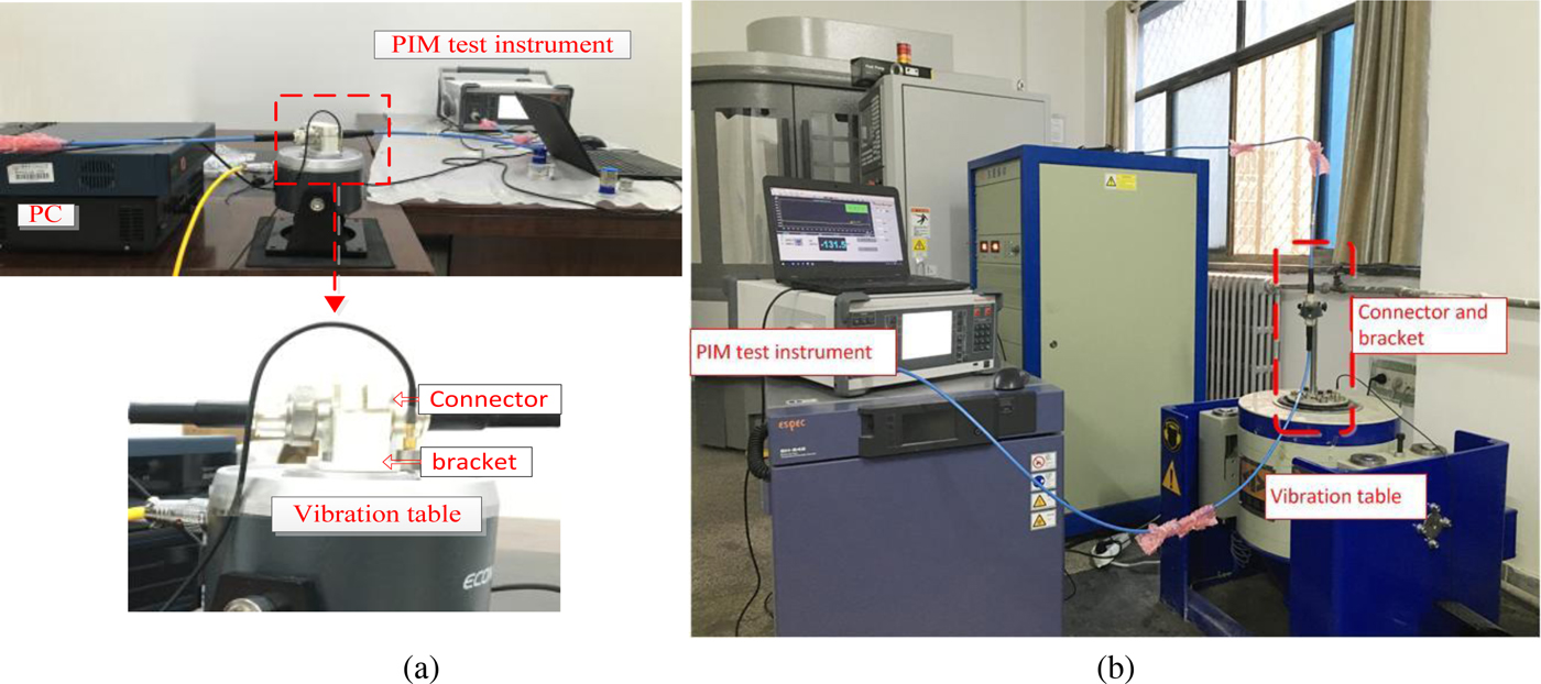
Fig. 2. Vibration experimental system: (a) horizontal arrangement test system; (b) vertical arrangement test system.
A TAYLOR HOBSON PGI1200 surface contour grapher, which is optical measurement method, is adopted to measure the rough surface contour of the DIN (7/16) connector.
The input frequencies in two-tone test are f 1 = 2620 MHz and f 2 = 2690 MHz. The third-order PIM with frequency 2f 1 − f 2 = 2550 MHz was measured at ambient temperature. Eventually, the calibrations of all instruments were accomplished.
Experimental results
As shown in Fig. 3(a), a CAD model of the connector is built for FEM analysis. Analysis operations include setting the contact element, meshing, specifying the boundary conditions, fixing one end and applying stress on the another end in ANSYS software. Then, the spectrum analysis is applied for finite-element calculation. Because of the skin effect, the roughness and mechanical properties of silver-plated surface are discussed in the experiment. In FEM model, the material is silver whose modulus of elasticity is 73.2 GPa, Poisson ratio is 0.38, density is 10.5 g/cm3, heat expansion coefficient is 1.95 × 10⁻⁶ K-1 and resistivity is 1.65 × 10⁻⁸ Ωm.

Fig. 3. A finite-element model of connector and its contact stress simulation. (a) CAD model of connector. (b) Simulation result of finite-element model in tightening torque = 10 Nm.
According to the parameters of material property and the experiment conditions, the contact stress of contact element is simulated for 10 Nm applied load and the results are shown in Fig. 3(b).
In our experiment, the surface roughness of the male connector and the female connector were measured separately. The one-dimensional contact surface scan of a new connector is shown in Fig. 4, and the surface roughness parameter r a measured by PGI1200 is 6.628 × 10⁻⁷ m. Through the power spectral density method, we can obtain the fractional parameter D of WM model by equations (11)–(17). In addition, in order to get the power spectral density of the data, we process the one-dimensional contact surface scan data in Fig. 4 by Fourier transform. Then, Fig. 6 is generated via the logarithmic transformation on S(k) and k. Considering the characteristic of impulse function δ(*), we extract the peak values from Fig. 5 and fit a straight line based on the least square method. Thus, the fractional parameter D of WM model is extracted from the measured data. The slope of straight line shown in Fig. 5 is −0.8996 and fractional roughness D = 2.5502 calculated by equation (17). In the contact analysis of connector, based on the Greenwood-Williamson model [Reference Jiang, Li, Ma and Wang24], the contact between two rough surfaces can be regarded as the contact between a smooth surface and a rough surface with equivalent material parameters. Then, the contact properties of the connector are obtained through FEM analysis.

Fig. 4. One-dimensional contact surface scan for a new male connector.
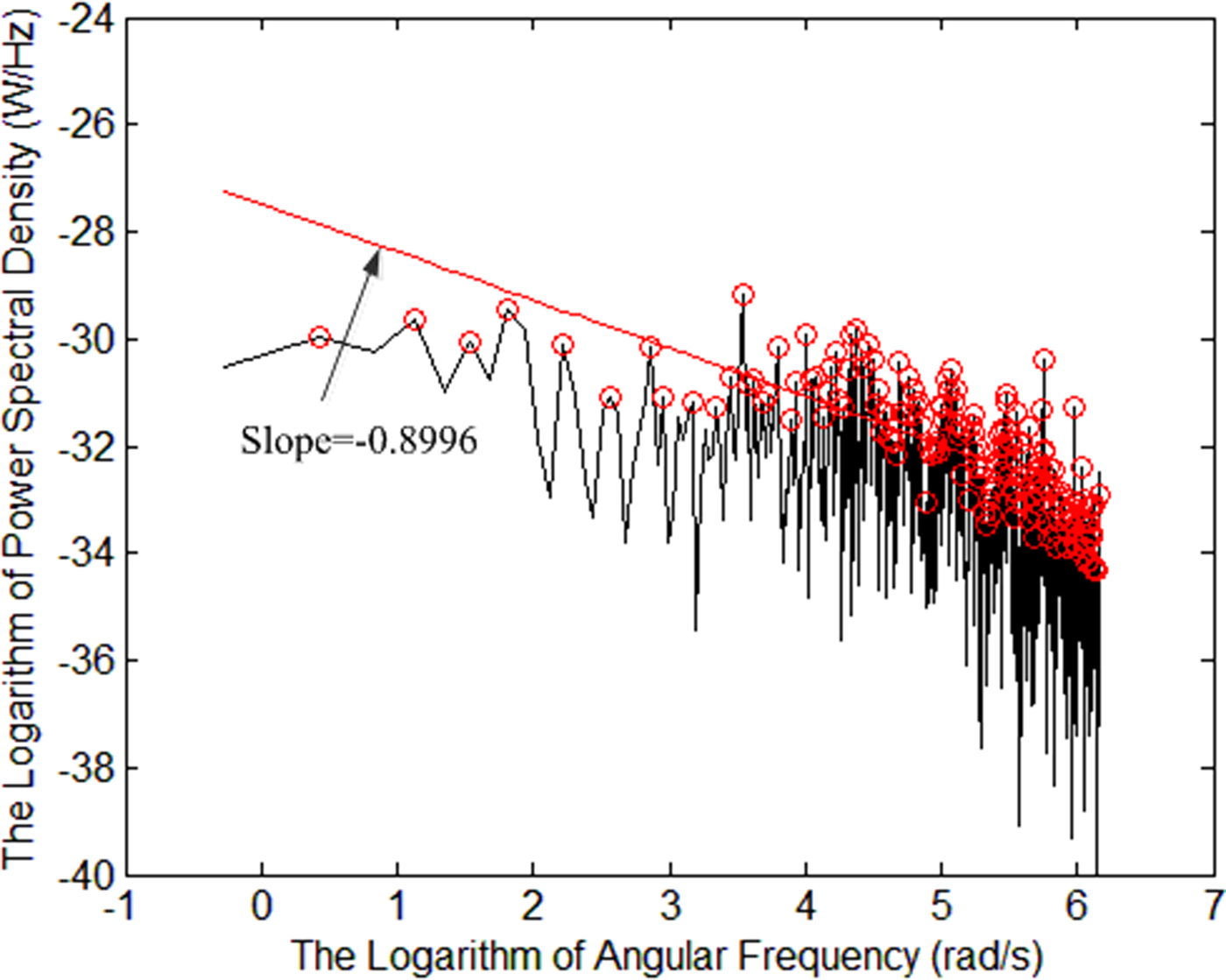
Fig. 5. Parameter identification of fractional roughness of contact surface for a new connector.

Fig. 6. Measured values of third-order PIM power levels for vibrational frequencies with different input powers. (a) Horizontal arrangement test, (b) Vertical arrangement test.
Effects of micro-vibration frequency
In vibration test, we have two forms of vertical and horizontal arrangements and six frequencies of micro-vibration adopted in the experiment, they are 0, 50, 100, 200, 300, and 400 Hz. 1 g acceleration and 10 Nm tightening torque are applied on the connector. The input power includes 36.99, 40.00, 41.76, 43.00, and 43.98 dBm. In the measurement system, the PIM analyzer, the test cable and the termination are low PIM equipment. The measurement system was calibrated to decrease the interference of other PIM sources. Due to the errors of measurement system, the same working condition is measured for five times and the average value is presented. Figure 6 shows the measured results of the third-order PIM power levels for vibrational frequency with different input powers. In every PIM test, according to the error processing criterion, for all measured PIM values, if the measurement error is 3 times larger than the standard error, the singular PIM value can be deleted.
From Fig. 6, it is obvious that the measured third-order PIM power levels in vertical arrangement are higher than that in horizontal arrangement generally. And the measured third-order PIM power levels increase with input power no matter which kind of arrangement forms. Based on the FEM analysis of connector, the variation of contact pressure with vertical vibration is larger than that with horizontal vibration. Thus, the third-order PIM power levels with the vertical arrangement are higher than that with a horizontal arrangement in general. However, when the frequency >50 Hz, the micro-vibration frequency has little effect on PIM. Comparing with microwave frequency, the effect of vibration frequency is negligible. PIM power level mainly depends on the input powers.
To reveal the differences between vibration and static environments, we measured the surface contour graph of a worn connector. The graph is shown in Fig. 7 and the parameter identification of fractional roughness is shown in Fig. 8.

Fig. 7. One-dimensional contact surface scan for a worn male connector.
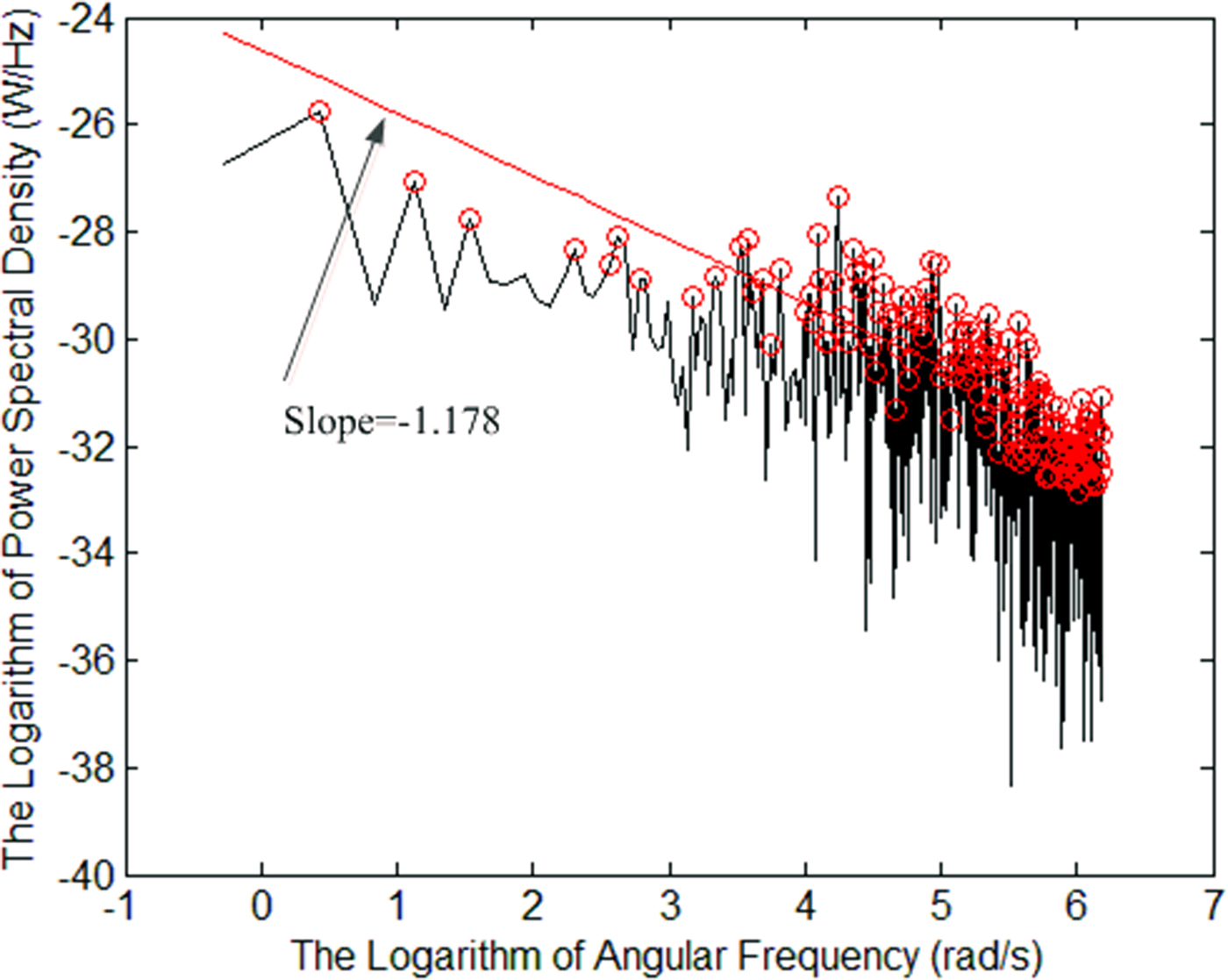
Fig. 8. Parameter identification of fractional roughness of contact surface for a worn connector.
The measured R a is 9.225 × 10⁻⁷ m, the slope is −1.178 and D = 2.411, the FEM model is constructed to reveal the effect of vibration on contact status. A periodic change in contact pressure will result in a change of PIM power levels. In our measurement system, the PIM power levels are measured every 5 s. Because the vibration frequency is much higher than test frequency, the PIM transients change is not possible to measure in our measurement system.
Furthermore, we tested the third-order PIM power levels for different input powers. The acceleration is 1 g and the vibration frequency is 400 Hz. For the constant torque, the measurement is done with only one connector in different input powers. According to the above parameters, we present the results of measured and calculated values in Fig. 9. To illustrate the effect of vibration on PIM, the variation of PIM calculated value with vibration is shown in Fig. 9. The lower solid line is the calculated values without vibration and the upper dashed lines are the calculated values with vibration. It is obvious that the values of third-order PIM power levels increase with the input powers. Furthermore, for the preloaded connectors, the variation of PIM power levels with vibration is generally much larger than that without vibration. On the other hand, values of PIM with vibration are greater than those without vibration generally. This phenomenon also verifies that the change of roughness is an important reason of PIM deterioration in vibration.
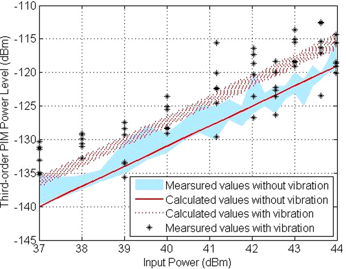
Fig. 9. Comparison of measured and calculated values of third-order PIM power levels with different input powers.
Effects of micro-vibration tightening torque
In Fig. 10, the measurements were done with new connectors for different preload, respectively, the lower solid line is the calculated values without vibration and the upper dashed lines are the calculated values for 400 Hz vibration frequency with 1 g acceleration, these data indicate that the micro-vibration may cause PIM to deteriorate. It can be seen from Fig. 10 that for the loose contact connectors, the variation of PIM power levels is larger than that for the preloaded connectors, whether or not to apply the vibration load. As the tightening torque increases, the area of the contact surface of the coaxial connector increases, while PIM value deduces. When the tightening torque is over 10 Nm, the contact stress calculated by ANSYS is beyond the yield limit of contact materials, and occurring plastic deformation, thus PIM is deteriorative.

Fig. 10. Comparison of measured and calculated values of third-order PIM power levels with different tightening torques.
In actual test, the measured values of PIM are fluctuant. Especially in micro-vibration environment, we have to give a range of measurement value with vibration and some points without vibration. The calculated values by the proposed method fall into the range of measurement results.
Effects of micro-vibration acceleration
In order to investigate the PIM power levels with different acceleration, the preloaded torque is 10 Nm, input power is 37dBm, the vibration frequency is 400 Hz. The small spacing accelerations (0, 0.2, 0.4, 0.6, 0.8, 1 g) and the large spacing accelerations (0, 1, 2, 3, 4, 5 g) are conducted on connector respectively by vibration table. The measurements were done with new connectors for different acceleration loads, respectively.
As shown in Figs. 11 and 12, the red dotted line is the mean values of measured power levels, solid blue lines are the distribution range of measured values. It is obvious that third-order PIM power levels and their variation increases with the acceleration. When the acceleration value is small, the increment of PIM power levels is not significant from Figs. 11(a) and 12(a). From Figs. 11(b) and 12(b), the increment of PIM power levels with acceleration is obvious. The reason of this phenomenon is the different vibration accelerations which lead to the different degrees of wear and the change of surface contour. Therefore, PIM distortion is higher with greater acceleration.
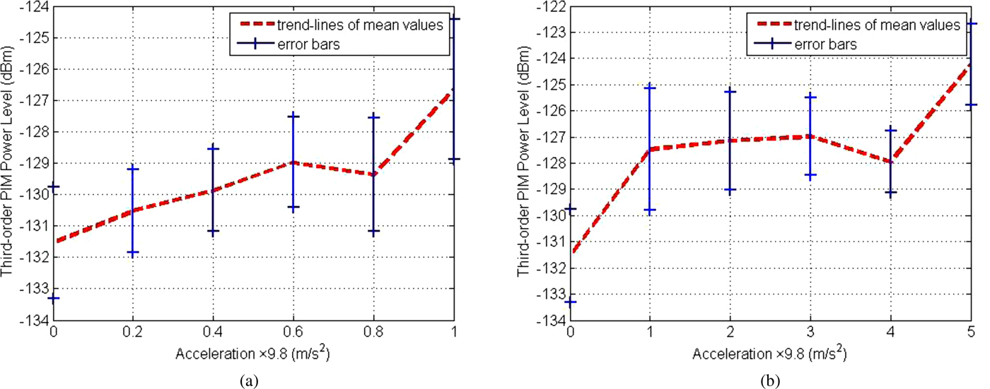
Fig. 11. Measured values of third-order PIM power levels with horizontal vibrational acceleration. (a) The small spacing accelerations, (b) The large spacing accelerations.
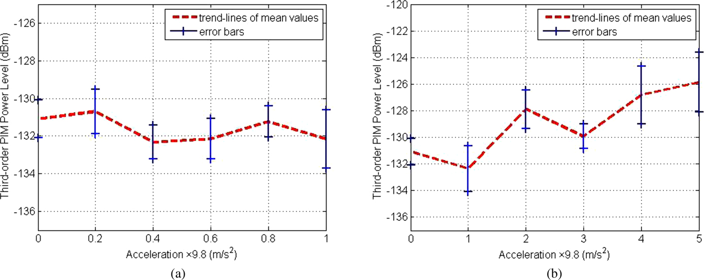
Fig. 12. Measured values of third-order PIM power levels with vertical vibrational acceleration. (a) The small spacing accelerations, (b) The large spacing accelerations.
Effects of micro-vibration duration
Finally, PIM degradation with the time of micro-vibration is investigated. The preloaded torque is 10 Nm, input power is 37dBm, the vibration frequency is 400 Hz and acceleration is 1 g. The measurement was done with one new connector, the third-order PIM power levels were measured for five times with 1 hour interval, the sampling time is 5 s.
As shown in Fig. 13, PIM power levels degrade with vibration duration. In a vibration environment, the relative motion of asperities will arise on the contact surface of the connector. This process leads that the surface of the plated metal is worn out and the base metal will be exposed, on the one hand, the effective contact area reduces and the constriction resistance increases. On the other hand, the base metal will be covered by a layer of insulator rapidly and the equivalent impedance increases further. Compared to preload, surface roughness, acceleration, and input power, the effect of micro-vibration duration is smaller.
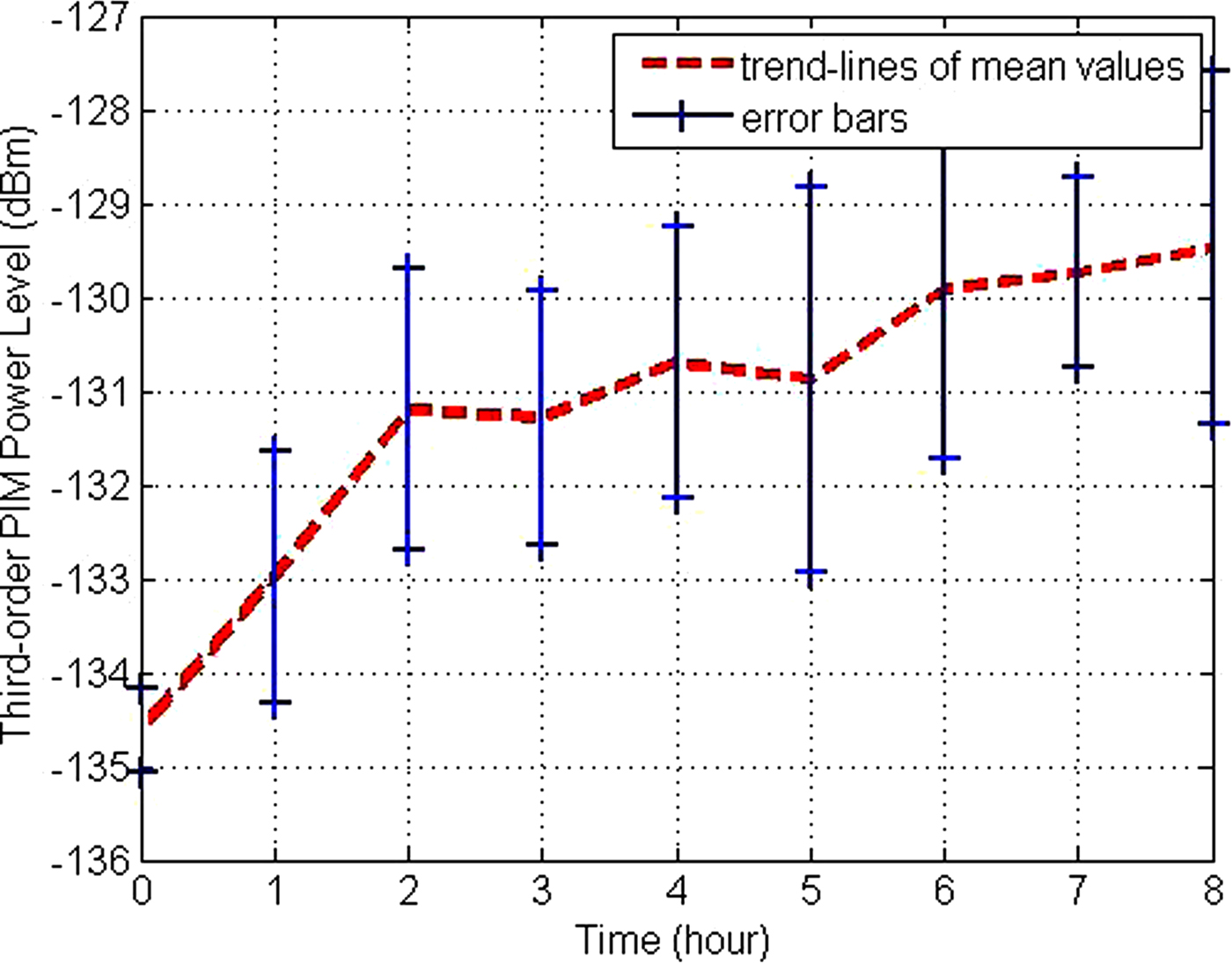
Fig. 13. Measured values of third-order PIM power levels with different vibrational duration.
Conclusions
Mechanical factors, such as contact roughness, contact stress and vibration, plays an increasing role in the electrical properties of connector. Therefore, this paper presented a method to identify parameters of surface roughness and calculated PIM of the DIN (7/16) connector based on the WM model. The paper reveals the effects of these mechanical factors on the third-order PIM power levels. Finally, we summarize some rules:
(1) For the short-time vibration, the micro-vibration frequency has little effect on PIM;
(2) When the contact stress exceeded the yield limit of the material, PIM would deteriorate;
(3) When the acceleration increases, the contact stress of the contact surface is greater;
(4) As time goes on, the degree of wear and corrosion of the contact surface lead to deterioration of PIM, simultaneously, electrical reliability gets worse.
Thus, some suggestions are as follows:
(1) When assembling the instrument, the metal particles and corrosion on the surface need to be cleaned;
(2) During the use of the connector, it was effective to reduce the external vibration, mechanical stress, and time of assembling and disassembling connectors;
(3) Installing connectors need to keep the appropriate torque.
Author ORCIDs
Tuanjie Li, 0000-0002-5426-8120
Acknowledgement
This research was supported by the National Natural Science Foundation of China (Grant No. 61801175).
 Tuanjie Li received his Ph.D. degree from Xi'an University of Technology in 1999. He is now a professor and Ph.D. supervisor at school of Mechano-Electronic engineering, Xidian University. His main research interests are space deployable structures and passive intermodulation.
 Mingtai Li received his Diploma in 2016 from Zhengzhou University. He is now a master of mechanical engineering in Xidian University. His current research interests include microwave technique and passive intermodulation.
 Wangmin Zhai received his Diploma in 2017 from Xidian University. He is now a master of mechanical engineering in Xidian University. His current research interests include microwave technique and passive intermodulation.
 Jie Jiang received her Ph.D. degree from Xidian University in 2016. She is now a teacher at Honghe University. Her current research interests include microwave technique and passive intermodulation.


