Microwave sensor characteristics

A microwave sensor for surface and subsurface imaging is designed based on two key points: (1) to have a sensor with high sensitivity, quality factor of the sensor should be high as much as possible. For this goal, a cavity resonator in the sensor structure is used to minimize the reflection coefficient; (2) to improve the image resolution as much as possible, the sensor tip should be sharpest.

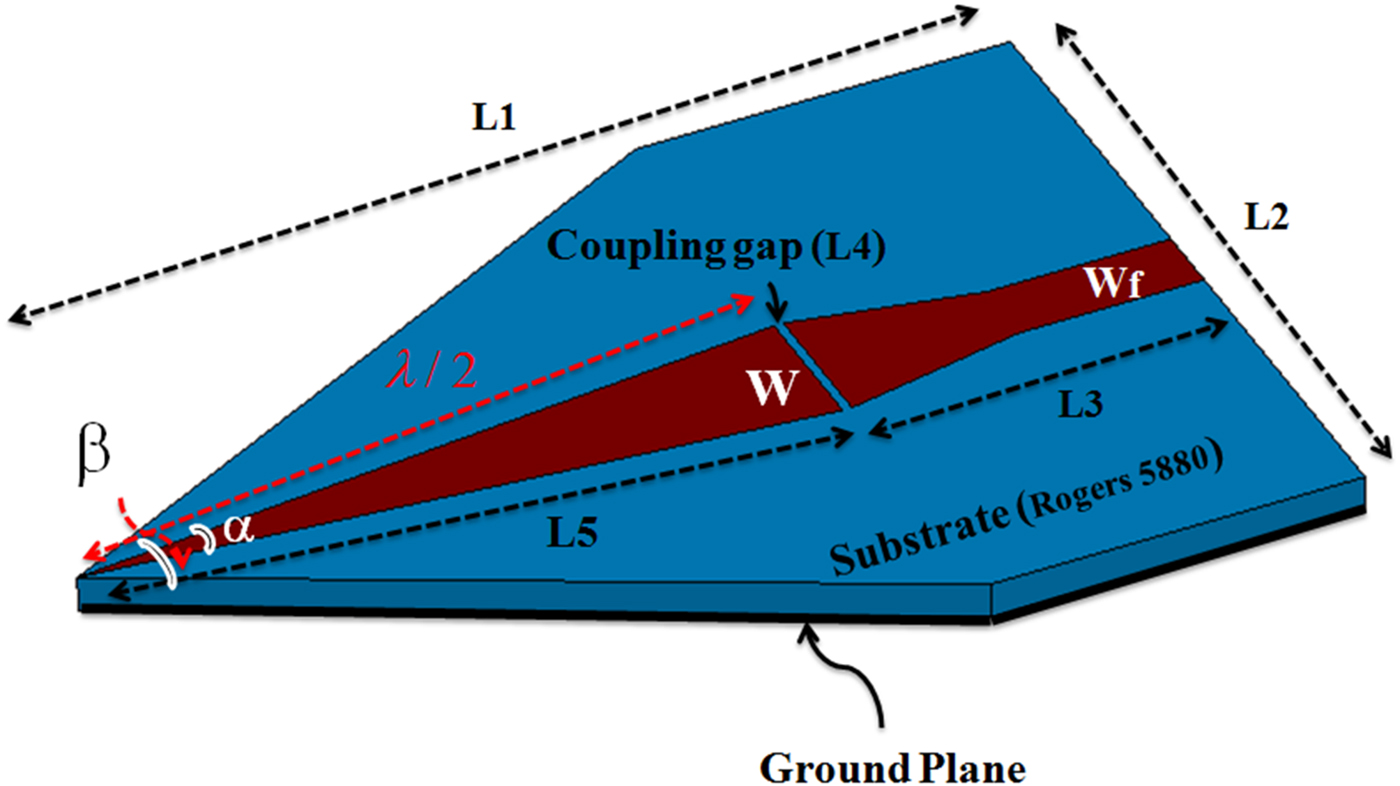
Geometry of a microwave sensor with λ/2 length of a 50 Ω open-circuited microstrip line is shown in Fig. 1. This sensor is design for the resonance at 13.5 GHz. The reason for choosing this frequency is to compromise between the penetration depth of the sensor and the resolution of the raw images. In other words, because the purpose is imaging of the subcutaneous masses, a frequency that can detect the hidden objects in the images with acceptable resolution and without any damage to the tissue is selected. The practical principle of a sensor using microstrip resonator is described in [Reference Pozar29, Reference Tabib-Azar, Katz and LeClair30]. Substrate of this structure is RT/duroid 5880 (ε _r = 2.2, tan(δ) = 0.0009) with a thickness of 0.8 mm.

Fig. 1. Geometry of a microwave sensor.

Design of the sensor is performed in two steps. First, the effect of two important parameters including tip sharpness (α) and size of the coupling gap on the sensor performance is numerically investigated using Ansoft HFSS software. The sharp angle (α) and the coupling gap size in order to have minimum of the return loss are achieved 11.2° and 0.2 mm, respectively. Final dimensions of the sensor are shown in Table 1. Quality factor of the sensor is obtained 5270.

Table 1. Dimensions (mm) of the sensor

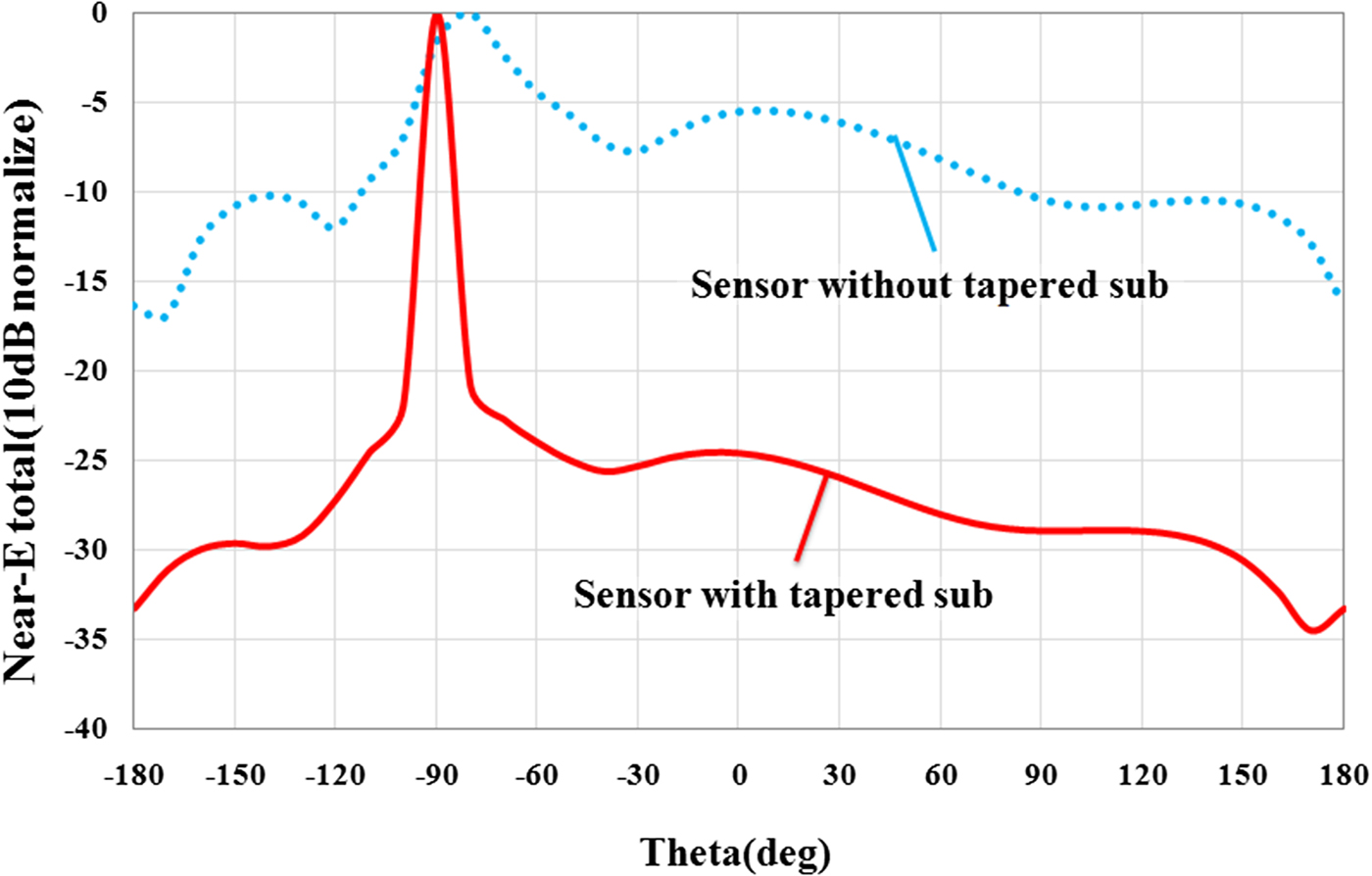
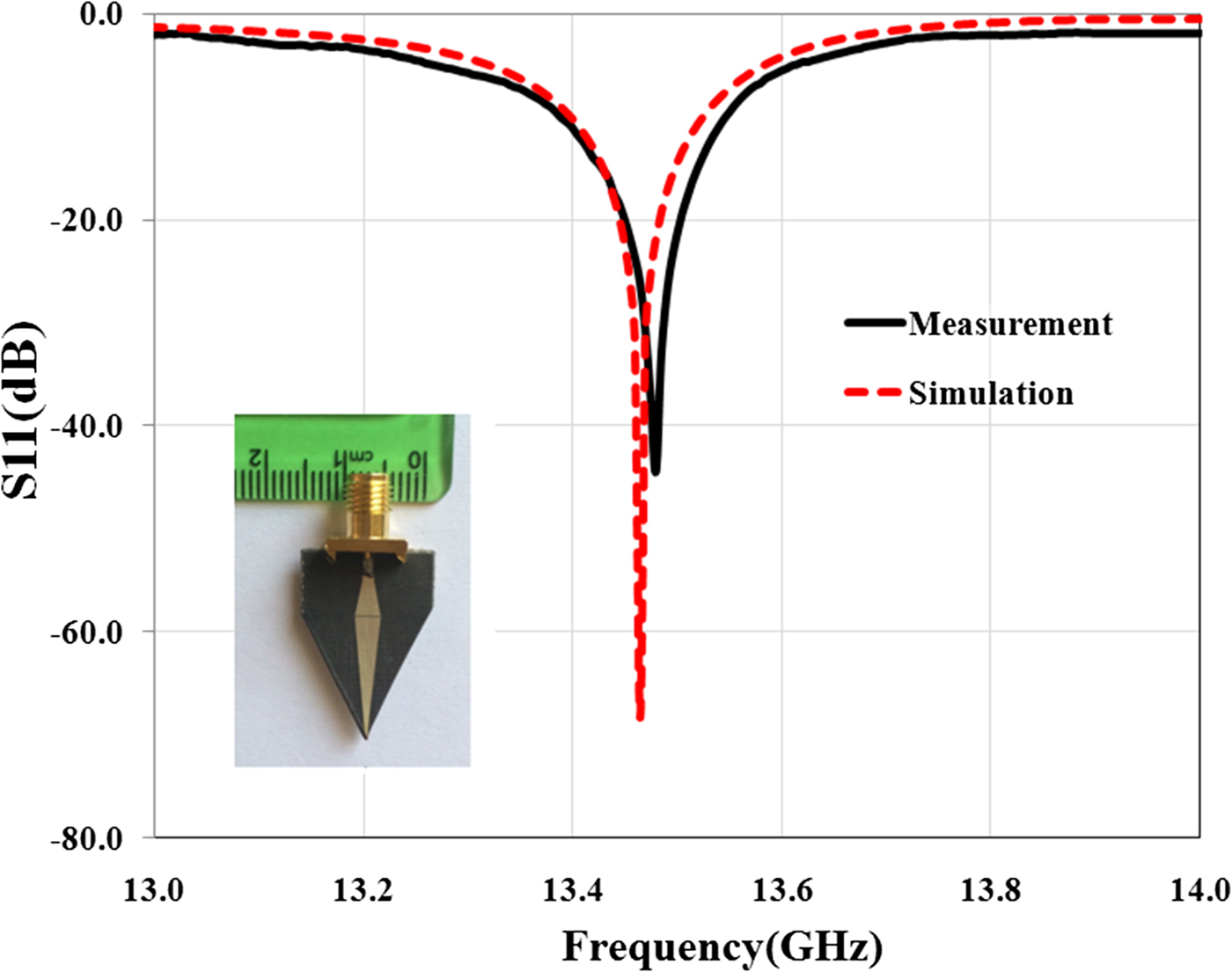
In the second step of sensor design, for reducing the side lobe level and focusing energy on the tip as much as possible, substrate and ground plane at the sensor tip is cut with different angles. Simulation results show that the angle (β) to have the highest field strength at the sensor tip is 53.4°. This cutting does not have effect on the quality factor of the sensor and only shifts slightly the resonant frequency. But near-field pattern of the sensor is significantly oriented on the sensor tip direction as shown in Fig. 2. Photograph of the manufactured sensor, simulation, and measurement results of the sensor's reflection coefficient are shown in Fig. 3.

Fig. 2. Rectangular near-field pattern of the sensor at 13.5 GHz (H-plane).

Fig. 3. Reflection coefficient of the sensor and photograph of the manufactured sensor.

Operation principles and background theory

When the microwave sensor is placed in the vicinity of a material under test (MUT), dielectric properties of MUT affect the quality factor (Q) and the resonant frequency (fr) of the sensor (Fig. 4(a)). These changes depend on the electromagnetic properties as well as the effective area of the sensor tip (A _eff; A _p) and the distance between MUT and the sensor tip (d _s). If the effective area of the sensor tip and distance between MUT and the tip is fixed, the sensor can scan the MUT and variations in the MUT's electromagnetic properties can be recorded [Reference Tabib-Azar, Katz and LeClair30].

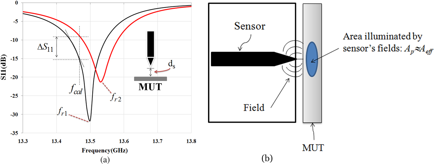
Fig. 4. (a) Resonant frequency and amplitude of the reflection coefficient is changed when the sensor is placed in front of the MUT. (b) Interaction between near-field sensor and MUT.

The electromagnetic properties of an MUT are a function of free carrier concentration, permeability, and permittivity. In human and biological tissues, the amounts of humidity and ionic species have a significant impact on its conductivity. Near-field microwave sensor can map these parameters and their density variations, which have effect on the permittivity [Reference Tabib-Azar, Katz and LeClair30]. There are different signal detection methods for monitoring the electromagnetic properties of a material using a near-field sensor. As shown in Fig. 4(a), when the operation frequency at f _cal (as calibration frequency) is fixed, the change in amplitude and phase of the reflection coefficient can be monitored. Calibration frequency (f _cal) is usually selected by the frequency where the reflection coefficient of the sensor has the maximum change for a given range of parameters in a material. Since the resonant frequency varies during the scan of material, the frequency shift (Δf) also can be detected.

As shown in Fig. 4(a), given a change in the reflection coefficient ΔS ₁₁ per a small change of Δd _s in the distance between an MUT and the sensor tip, we can only detect ΔS ₁₁ if it is equal to or larger than the combined noise produced by the detector. The signal-to-noise ratio is an arbitrary requirement that it can be improved by using synchronous detection methods. If relationship between ΔS ₁₁ and Δf in Fig. 4(a) is defined by:

(1)$$\Delta S_{11} \approx \left. {\displaystyle{{\Delta S_{11}} \over {\Delta f}}} \right \vert _{\,f_{cal}} \times \Delta f.$$

Then $(\Delta S_{11}/\Delta f)_{f_{cal}}$ is defined as the sensitivity of the near-field sensor at f _cal and can be noted by S _cal. Moreover, the minimum-detectable signal (MDS) can be defined as the smallest change in the input that produces an output (ΔV _out = ΔS ₁₁V _in) equal to the rms value of the noise V _nrms. Also, if ΔS ₁₁/Δfis written as ΔS ₁₁/Δf = ΔS ₁₁/Δd _s × Δd _s/Δfthen we can write [Reference Tabib-Azar31]:

(2)$$\Delta S_{11} = \displaystyle{{V_{nrms}} \over {V_{in}}},$$

and

(3)$${\rm MDS} = \Delta d_s = \displaystyle{{V_{nrms}/V_{in}} \over {S_{cal}S_{d_s}}}.$$

Here S _ds is Δd _s/Δf and Δd _s is the smallest change in the stand-off distance. Equation (3) clearly shows that by maximizing of S _ds and S _cal, the MDS will be improved. S _cal is related to the quality factor of the near-field sensor, while S _ds is determined by the interaction between sensor and MUT.

Interaction between near-field sensor and MUT is shown in Fig. 4(b). The field patterns at the surface of the MUT are spread over an area denoted by A _eff ≈ A _p, where A _p is the physical area of the sensor tip and A _eff is an effective interaction area [Reference Tabib-Azar31]. It is very important to differentiate between variations in the distance and changes in the electromagnetic properties of the MUT. In practice both the MUT conductivity and distance between the sensor and the MUT will change during its scan. Fortunately, effect of the variations in distance appears exponentially on the sensor's output while the MUT's non-uniformity usually occurs over larger length scales.

We modeled the strip-line resonator (open-circuit transmission line) by a series RLC circuit near its resonance frequency (Fig. 5(a)). When an MUT is placed near the tip, its electromagnetic properties are coupled to the RLC circuit through a coupling capacitor. For simplicity, dielectric MUTs are modeled in Fig. 5(b). In these figures, R _P, L _P, and C _P are the intrinsic circuit parameters of the strip-line resonator; C _c models the coupling capacitance of the air gap between a tip and an MUT; L _MUT, C _MUT, and R _MUT model the microwave properties of an MUT. The resonant frequency shifts in the presence of an MUT near a sensor tip. From these circuit models, it is clear that a shift in resonant frequency depends on both complex conductivities of the MUT and on the stand-off distance [Reference Chen32].

Fig. 5. (a) Series of lumped RLC models of a microwave sensor. (b) Circuit model in the presence of a dielectric MUT.

If the coupling capacitance C _c in Fig. 5(b) is defined by:

(4)$$C_c = \displaystyle{{\varepsilon _0A_{eff}} \over {d_s}},$$

then we can calculate S _ds as:

(5)$$S_{ds} = \displaystyle{{\varepsilon _0A_{eff}f_0} \over {d_s(Cpd_s + \varepsilon _0A_{eff})}}.$$

For typical values of a sensor (A _eff ≈ A _p ≈ 4 × 10⁻⁴ cm², d _s = 2 mm, f ₀ = 13.5 GHz, Q = 5270, C _p = 7.3 pF, C _c = 12 pF) S _ds becomes:

$$\eqalign{S_{ds}& = \displaystyle{{8.85 \times {10}^{ - 14} \times 4 \times {10}^{ - 8} \times 13.5 \times {10}^9} \over {2 \times {10}^{ - 3}(7.3 \times {10}^{ - 12} \times 2 \times {10}^{ - 3} + 8.85 \times {10}^{ - 14} \times 4 \times {10}^{ - 4})}} \cr & = 3.2575 \times 10^6.}$$

It should be noted that S _ds has an inverse relationship with distance square between a sensor and an MUT (/ds²). This means that dependency will be exponential if a sensor is very near to an MUT.

Assuming that the resonator is matched to the characteristic impedance of the feed-line at calibration frequency, S _cal is calculated by [Reference Tabib-Azar31]:

(6)$$S_{cal} \approx s\displaystyle{{\sqrt 2 Q} \over {\omega _{cal}}}\left( {1 - \displaystyle{{\Delta \omega} \over {\omega _{cal}}}} \right),$$

where ω = ω _cal + Δω and Δω/ω _cal < 1 and s = −1 if ω < ω _cal and s =  + 1 if ω > ω _cal. Therefore, as we expect, the sensor sensitivity is directly proportional to its quality factor. For the near-field sensor in this study, S _cal is calculated 4.4 × 10⁻⁸.

Using equations (5) and (6) in equation (3), we have:

(7)$$MDS = \Delta d_s \approx \displaystyle{{V_{nrms}} \over {V_{in}}}\displaystyle{{2\pi d_s(C_pd_s)} \over {Q(1 - \Delta f/f_{cal})\varepsilon _0A_{eff}}}.$$

For typical values of S _cal and S _ds in equations (5) and (6), a numerical value of 0.75 mm is obtained for MDS. The circuit approach that is used in defining the coupling capacitance is only an approximation and it does not account for the decay of electromagnetic fields near the tip. Our experimental set-up and procedure for microwave measurements are discussed in the next section.

Experimental set-up and procedure

In this section, first, a simulation study is investigated by HFSS software to show the capability of the sensor for the diagnosis of different biological tissues. For this purpose, according to the experiments, the near-field sensor is placed in front of different tissues such as skin (ε _r = 27.5-j16 at 13.5 GHz), fat (ε _r = 3.6-j0.6 at 13.5 GHz), and muscle (ε _r = 32.2-j25 at 13.5 GHz). The dielectric values for different tissues were interpolated from the values given by Gabriel et al. [Reference Gabriel, Lau and Gabriel33]. As shown in Fig. 6(a), quality factor (Q) and resonant frequency (f _r) of the sensor are affected by the electromagnetic properties of the tissues. The simulation results in Fig. 6(a) show that the sensor will be able to detect the different tissues in the experiments. Moreover, the simulated near E-field (by HFSS) amplitude distribution at 2 mm at the frequency of 13.5 GHz in front of fat masses along the muscle tissue shows that the near-field focal area is substantially confined in space (Fig. 6(b)). Also, by increasing the distance, the energy focus reduces. Therefore, the stand-off distance to achieve the images with good resolution is 2 mm.

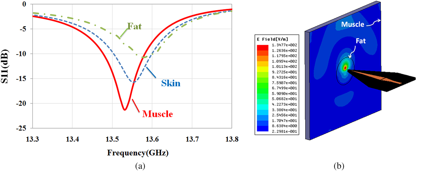
Fig. 6. (a) Reflection coefficient of the sensor in the presence of different biological tissues at 2 mm stand-off distance. (b) E-field amplitude at 2 mm stand-off distance in front of fat mass along the muscle tissue.

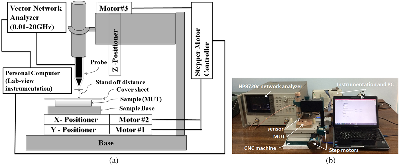
The experimental set-up used in this work is shown in Fig. 7. As mentioned, a microstrip resonator is used as a sensor that is connected to a 0.01–20 GHz vector network analyzer via an RF cable. The near-field sensor is fixed on the z-axis vertically to the MUT at 0.1 λ stand-off distance away from the MUT and two-step motors move the MUT in the x and y directions. As mentioned before, since the sensor tip does not make contact with the MUT, the MUT's surface can have a variety of characteristics, including being sticky or immersed in a dielectric fluid. Before measurement, the system is calibrated. To perform the calibration, distance between probe and MUT (d _s) is changed to minimize the magnitude of the reflection coefficient. Then this distance is kept constant along our measurements (about 2 mm) and frequency of the minimum magnitude of S ₁₁ is considered as calibration frequency (f _cal). During MUT scanning, magnitude of S ₁₁ at calibration frequency and frequency shift (Δf) are recorded to detect the visible and hidden objects. Also, in our measurements, a National Instrument Data Acquisition with their Lab-View software is used to control the stepper motors and to acquire the measurement data. The movement step during all scanning measurements is 1 mm. Moreover, all experiments are carried out at room temperature (23 °C).

Fig. 7. (a) Schematic representation and (b) photograph of our experimental set-up.

Experimental results and discussion

Since “lipoma” is a benign tumor composed of fat tissue and it is the most common benign form of soft-tissue tumor, in this section, a measurement scenario is defined based on the surface and subsurface detection of “lipoma”. Moreover, for results validation, an image of “lipomas” with different sizes and distances below a skin layer is obtained. Finally, our proposed sensor capability for skin cancer detection is studied using an artificial skin model.

Surface and subsurface detection of “lipomas”

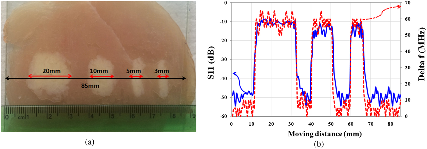
In this section, in order to study the presented microscope features, resolution of the proposed near-field sensor for the diagnosis of “lipomas” is measured. Therefore, two experiments are applied. Initially, as shown in Fig. 8(a), four “lipomas” with a size of 20, 10, 5, and 3 mm are located orderly along the muscle tissue and the proposed sensor scans a vector of 85 mm length along them as well. Thickness of the tissues is considered about 2 mm for fat and muscle tissues and 1 mm for skin tissue. In all experiments, the tissues roughness is not considered, and to keep the stand-off distance between probe and tissues constant, a transparent plastic sheet (as cover sheet) is placed on the tissue. Subsequently, in each experiment, two parameters including the amplitude of reflection coefficient and the frequency shift are measured.

Fig. 8. (a) Photographs of “lipomas” with different sizes. (b) Magnitude of reflection coefficient and frequency shift (Δf).

Measurement results of S ₁₁ in Fig. 8(b) show that the proposed sensor is able to detect the “lipomas” with sizes larger than 3 mm.

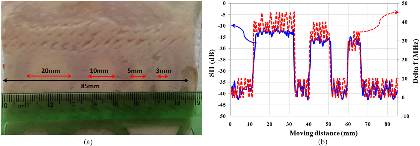
In the second experiment, for subsurface imaging, different sizes of fat masses are placed along the muscle tissues below the skin. As shown in Fig. 9(a), four “lipomas” with a size of 20, 10, 5, and 3 mm are located below the skin, respectively, and scanned by the proposed sensor. Fig. 9(b) shows the measurement results. Results show that the sensor is able to detect hidden “lipomas” at a minimum size of 5 mm. It is noted that in the medical research, masses that are grown larger than 5 mm is important for the diagnosis from cancerous tumor [Reference Thompson34]. Therefore, the proposed sensor is suitable for detecting subcutaneous masses and distinguishing them from the cancerous masses in the early stage.

Fig. 9. (a) Photograph of “lipomas” with different sizes below skin layer. (b) Magnitude of reflection coefficient and frequency shift (Δf).

Image realization

For results validation, an image of the hidden “lipomas” in different sizes and spaces is obtained. As shown in Figs 10(a) and 10(b), the “lipomas” with different sizes are placed along the muscle tissues below a skin layer and the sensor scans a matrix of 90 × 90 mm dimensions. The operation frequency is fixed at 13.5 GHz, where the image is obtained at 2 mm (λ/10) imaging distance. As the results shown in Figs 10(c) and 10(d), high-quality raw images of “lipomas” below the skin are achieved with an amplitude contrast of about 15 dB and a frequency shift contrast of about 60 MHz.

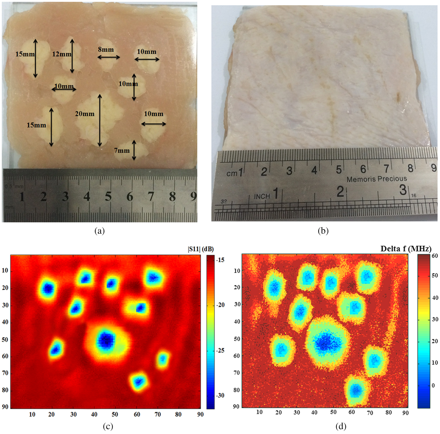
Fig. 10. Photograph of “lipomas” with different sizes, (a) without cover, (b) with cover by a layer of skin, and a microwave image from, (c) measurement of the S ₁₁ magnitude, (d) measurement of the frequency shift (Δf).

Detection of skin cancer using an artificial skin model

In all kinds of skin cancers, the amount of water content is increased, mostly, in the epidermis layer [Reference Suntzeff and Carruthers27]. The water content of malignant lesions is about 20% higher than the normal skin. But, many benign lesions are drier than normal skin [Reference Gniadecka35]. This difference in water content is expected to be readily detected in microwave measurements. At microwave frequencies, the dielectric properties of normal skin can be distinguished from those of lesions by measuring their reflection properties [Reference Zoughi28]. Previous studies [Reference Mehta22–Reference Taeb, Gigoyan and Safavi-Naeini24] show that the microwave reflection contrast between the malignant tumor and healthy skin is approximately similar to that of dry and wet skin. Also, these studies diagnose the malignant tissue from normal tissue by the coaxial sensor with low contrast (1–3 dB) because of low coupling between the sensor and the tissues.

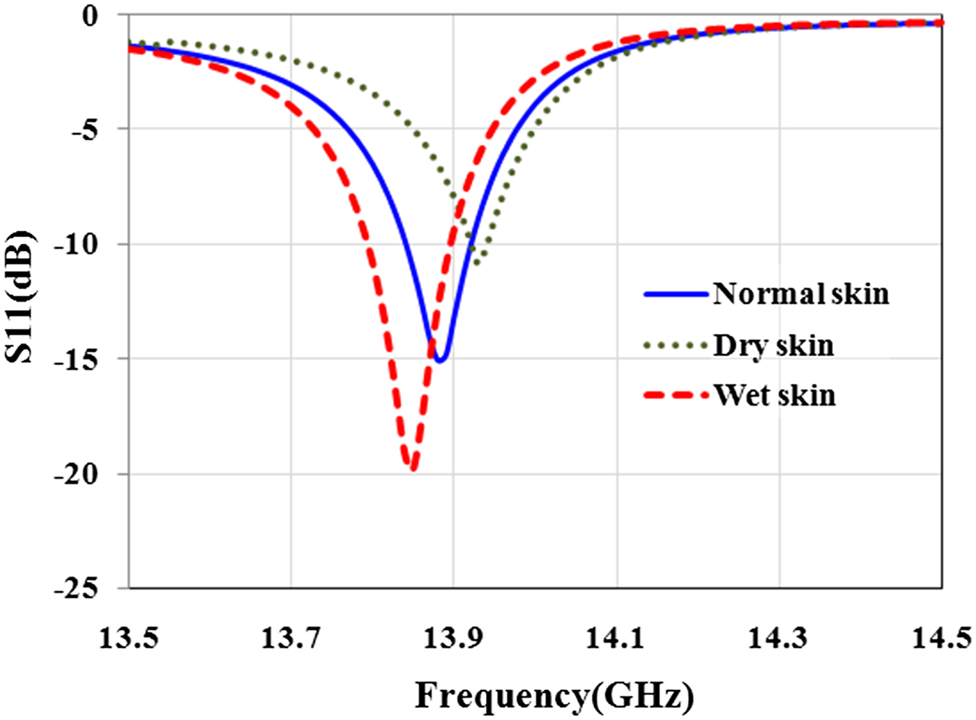
Before the experiment, a simulation was conducted to estimate the sensor's ability to detect the skin with different water content. For this aim, sensor is placed in front of dry (ε _r = 23.15-j16.08 at 13.5 GHz), normal (ε _r = 27.5-j16.11 at 13.5 GHz), and wet (ε _r = 29.64-j17.26 at 13.5 GHz) skin. Simulation results in Fig. 11 show that the sensor is able to diagnose the skin with different water content with high contrast.

Fig. 11. Effect of water content in the skin on the magnitude and resonant frequency of reflection coefficient.

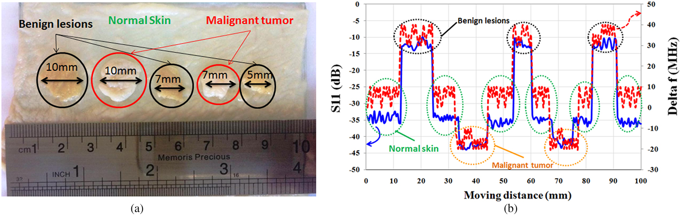
In the experiment, microwave properties of the healthy skin, malignant tumors, and benign lesions are modeled using layers of raw chicken skin with different water content. For this purpose, a piece of raw chicken skin is placed in a tank of water for ~20 min (representing melanoma). Another piece of the skin is placed in contact with air for 20 min (representing benign lesions). Moreover, a piece of normal skin (without contact with air and water) is considered as healthy skin. Then, as shown in Fig. 12(a), a few slices of melanomas and benign lesions are placed on the healthy skin and the sensor scans a vector along these tissues. This model is designed to represent skin cancer development at the early stages (http://www.cancerresearchuk.org,http://www.skincancer.org/melanoma) when only small, node-like tumors occur. Thickness of all layers of skin is about 1 mm and the size of skin slices (cancerous tumors) varies from ~5 mm (λ/4) to 10 mm (λ/2). The operation frequency is fixed at 13.5 GHz, where stand-off distance between sensor and skin is 2 mm (λ/10). Measurement results in Fig. 12(b) show that the sensor could accurately detect malignant tumor with about 10 dB contrast in magnitude and 30 MHz contrast in frequency shifts from healthy skin and with about 30 dB contrast in magnitude and 60 MHz contrast in frequency shifts from benign lesions. It is noted that if dimensions of the sensor scale down, other types of skin cancer such as basal cell carcinoma and squamous cell carcinoma will be characterized with super resolution at millimeter waves.

Fig. 12. (a) Artificial model to detect skin cancer at the early stage. (b) Magnitude of S ₁₁ and frequency shift (Δf).