


I. INTRODUCTION
Higher data rates and reliable communication systems are the main pillars for new technologies. Multiple-input–multiple-output (MIMO) systems are employed in current 4 G and future 5 G systems. The increase in the data rates and better reliability offered by MIMO relies on the number of uncorrelated channels available within the system. Among other factors, antenna design is also a contributing factor in inducing the correlation between channels and therefore must be characterized.
The correlation coefficient (ρ) is a performance metric defined to characterize and compare the performance of MIMO antenna systems in terms of how much correlation they will add within the channels. A low value for ρ is desired. Several methods were discussed in literature to evaluate ρ for MIMO antenna systems. First described in [Reference Vaughan and Andersen1], ρ between two antenna elements is defined as a function of the radiation pattern of each antenna element and the spatial power distribution of the signal in a propagation environment. In most of the subsequent methods for evaluating ρ, the spatial power distribution of the signal is considered uniform (i.e an isotropic environment). Thus, ρ is mainly a function of the radiation pattern of each antenna element. A simpler method for the computation of ρ is given in [Reference Blanch, Romeu and Corbella2]. This method used the S-parameters of the MIMO antenna system to find it. This method is derived under the assumption that the MIMO antenna system is lossless. In [Reference Stjernman3], an extension to N-elements is provided.
In practice, all printed antennas are lossy, thus using the S-parameter method to calculate ρ for such antennas results in wrong values. In [Reference Hallbjorner4], the effect of the total radiation efficiency is considered to estimate the worst possible correlation performance. In [Reference Vaughan and Andersen1, Reference Li, Lin, Lau and He5] it is shown that ρ has no relation with the radiation efficiency, hence ρ should be calculated from lossless S-parameters, which can be extracted from the measured S-parameters after calculating the losses in the antenna system. The challenge in this method is to calculate the loss resistance, which can be easily obtained if antenna systems can be represented by their equivalent circuits [Reference Li, Lin, Lau and He5]. The equivalent circuit method for serial and parallel circuits of antennas to calculate ρ are investigated and applied for two elements and only the series equivalent circuit was demonstrated on more than two element antenna systems that were symmetrically spaced. It should be noted that the effect of using multiple lossy antennas in close proximity on the efficiency was investigated in [Reference Yun and Vaughan6, Reference Yun and Vaughan7]. Large deviation between field-based and S-parameter-based methods were found in [Reference Razmhosseini and Vaughan8, Reference Bhattacharya and Vaughan9] when considering practical printed circuit boards (PCB) antennas. But no further analysis was conducted to compare and explain such deviations.
In this work, we analyze the performance of various ρ calculation methods that appeared in [Reference Vaughan and Andersen1–Reference Li, Lin, Lau and He5], when applied to high, moderate, and low efficiency (η) antennas. Three MIMO antenna types based on patches (low η), planar inverted F antennas (PIFA) (moderate η), and printed monopoles (high η) are used to draw the conclusions on the ρ calculation accuracy of these methods, their complexity and validity. This is chosen because most of MIMO antenna works in literature are derivatives of these three antenna types. A new meandered four-element PIFA-like antenna is designed and analyzed besides the half-circle monopole and the four-element patch-based MIMO antenna systems. All designs are fabricated and measured. In addition, we extended the method in [Reference Hallbjorner4] to cover N-ports as well as extended the parallel equivalent circuit method in [Reference Li, Lin, Lau and He5, Reference Li, Lin, Lau and He10] to cover more than two elements. A study on the affect of tilted beams on ρ calculations is also conducted for the first time. Based on this work, the usefulness and limitations of each of the four methods along with their validity are highlighted, which will help antenna designers when characterizing their MIMO antenna designs.
II. CORRELATION COEFFICIENT CALCULATION METHODS
A) Correlation coefficient calculation using the radiation patterns (method-I)
This method calculates ρ from the three-dimensional (3D) far-field radiation patterns for each pair of the antenna elements. For any wireless environment ρ is found using [Reference Vaughan and Andersen1]:
 $$\rho _{mn} = \displaystyle{{\int_{ - \pi }^\pi {\int_0^\pi {(XPRA_{\theta ,m}(} } \theta ,\phi )A_{\theta ,n}^ * (\theta ,\phi )p_\theta (\theta ,\phi ) + {\rm }A_{\phi ,m}(\theta ,\phi )A_{\phi ,n}^ * (\theta ,\phi )p_\phi (\theta ,\phi ))\sin \theta d\theta d\phi } \over {\sqrt {\delta _m^2 \delta _n^2 } }},$$
where
 $$\delta _n^2 = \int_{ - \pi} ^\pi \int_0^\pi (XPR\left \vert {A_{\theta, n} (\theta, \phi )} \right \vert ^2 p_\theta (\theta, \phi ) + \left \vert {A_{\phi, n} (\theta, \phi )} \right \vert ^2 p_\phi (\theta, \phi ))\sin \theta d\theta d\phi, $$
 $$\delta _m^2 = \int_{ - \pi} ^\pi \int_0^\pi (XPR\left \vert {A_{\theta, m} (\theta, \phi )} \right \vert ^2 p_\theta (\theta, \phi ) + \left \vert {A_{\phi, m} (\theta, \phi )} \right \vert ^2 p_\phi (\theta, \phi )){\rm sin}\theta d\theta d\phi, $$
A θ,m (θ, ϕ), A ϕ,m (θ, ϕ), A θ,n (θ, ϕ) and A ϕ,n (θ, ϕ) are the elevation and azimuthal radiated field components for elements n and m, respectively. ()* is the conjugate operator. XPR is the cross polarization discrimination factor showing the ratio between the vertically and horizontally polarized power components of the incoming wave, and p θ (θ, ϕ), p ϕ (θ, ϕ) are the angle of arrival power densities for θ and ϕ angles, respectively. For an environment with a uniform distribution of vertical and horizontal components of the incoming waves (i.e. isotropic environment, which is widely adopted in rich multipath scenarios where MIMO systems operate, and most works use this assumption in their derivations, thus to compare under the same assumptions, this scenario is adopted), ρ can be calculated using [Reference Vaughan and Andersen1]:
 $$\rho _{ij} = \displaystyle{{\left \vert {\int\!\! \int_{4\pi} \overrightarrow {F_i} (\theta, \phi ){\ast}\overrightarrow {F_j} (\theta, \phi )d\Omega} \right \vert} \over {\int\!\! \int_{4\pi} \left \vert {\overrightarrow {F_i} (\theta, \phi )} \right \vert d\Omega \int \!\!\int_{4\pi} \left \vert {\overrightarrow {F_j} (\theta, \phi )} \right \vert d\Omega}} $$
where * is the Hermitian product,
 $\overrightarrow {F_i} (\theta, \phi )$
and
$\overrightarrow {F_i} (\theta, \phi )$
and
 $\overrightarrow {F_j} (\theta, \phi )$
are the 3D radiated fields of the antennas when the ith and jth ports are excited and Ω is the solid angle. The envelope correlation coefficient (ρ
e
) can be approximated by squaring (4).
$\overrightarrow {F_j} (\theta, \phi )$
are the 3D radiated fields of the antennas when the ith and jth ports are excited and Ω is the solid angle. The envelope correlation coefficient (ρ
e
) can be approximated by squaring (4).
This method has one drawback, which is requiring measured 3D filed patterns of each antenna element. Thus, it might be relatively expensive (if no measurement chamber is available), and requires time in collecting the patterns at the frequency points of interest. However, this is the most accurate and exact method for ρ calculations, and can be applied on any number of antenna elements with any efficiency values. This method should be used all the time.
B) Correlation coefficient calculation using S-parameters (method-II)
In [Reference Blanch, Romeu and Corbella2], a relation between the radiated field (total power) and the port parameters (S-parameters) is demonstrated for
 $100\% $
efficient antennas working in isotropic environments. The method is valid only for finding ρ between two element systems. In [Reference Stjernman3], it was generalized for N-elements and is given by:
$100\% $
efficient antennas working in isotropic environments. The method is valid only for finding ρ between two element systems. In [Reference Stjernman3], it was generalized for N-elements and is given by:
 $$\rho _{ij} = \displaystyle{{ - \sum\nolimits_{n = 1}^N {S_{ni}^{\ast} S_{nj}}} \over {\sqrt {\left( {1 - \sum\nolimits_{n = 1}^N {\left \vert {S_{ni}} \right \vert ^2}} \right)\left( {1 - \sum\nolimits_{n = 1}^N {\left \vert {S_{nj}} \right \vert ^2}} \right)}}}, $$
where ρ ij is the correlation between elements i and j, S ni , and S nj are the S-parameters between each of the n various ports and elements i and j of MIMO antenna system.
This method has been used in most of the literature to find ρ. The advantages of this method are its fast and ease of use as it only depends on the port parameters of the antenna system. On the other hand, this method is unreliable when the radiation efficiency of the antenna elements is not
 $100\% $
and it does not account for non-uniform directive patterns that are seen in most practical antennas (it should be mentioned that this method does not account for the beam tilts that are the ones that affect the channel of the incoming signals, and thus has a direct effect on the achieved capacity of the system). Thus, this method usually underestimate the ρ values and should not be used.
$100\% $
and it does not account for non-uniform directive patterns that are seen in most practical antennas (it should be mentioned that this method does not account for the beam tilts that are the ones that affect the channel of the incoming signals, and thus has a direct effect on the achieved capacity of the system). Thus, this method usually underestimate the ρ values and should not be used.
C) Correlation coefficient calculation using S-parameters and radiation efficiencies (method-III)
This method gives more reliable calculations than using only the S-parameters because it considers the effects of the radiation efficiency, but instead of giving the exact value, it gives an upper bound for ρ. In [Reference Hallbjorner4], the calculation of ρ was derived for two-element MIMO antennas, and here we generalize it for N-elements as:
 $$\rho _{ij,max} = \displaystyle{{ - \sum\nolimits_{n = 1}^N {S_{ni}^{\ast} S_{nj}}} \over {\sqrt {\left( {1 - \sum\nolimits_{n = 1}^N {\left \vert {S_{ni}} \right \vert ^2}} \right)\left( {1 - \sum\nolimits_{n = 1}^N {\left \vert {S_{nj}} \right \vert ^2}} \right)\eta _{rad,i} \eta _{rad,j}}}} + \sqrt {\left( {\displaystyle{1 \over {\eta _{rad,i}}} - 1} \right)\left( {\displaystyle{1 \over {\eta _{rad,j}}} - 1} \right)}, $$
where η
rad,1 and η
rad,2 are the radiation efficiencies of the two antenna elements, and the second term in (6) represents the degree of uncertainty which is high when the radiation efficiencies are low, and thus the value of ρ can be >1. This method provides better accuracies compared with method-II, but once the efficiency goes below 60
 $\% $
the errors start increasing dramatically. The calculation of ρ using this method requires one extra measurement, which is the efficiency. This method does not account for the pattern shape or tilt, similar to method-II, and thus it is also unreliable and should be avoided. The extension of this method to N-element and the derivation of (6) is given in Appendix A.
$\% $
the errors start increasing dramatically. The calculation of ρ using this method requires one extra measurement, which is the efficiency. This method does not account for the pattern shape or tilt, similar to method-II, and thus it is also unreliable and should be avoided. The extension of this method to N-element and the derivation of (6) is given in Appendix A.
D) Correlation coefficient calculation based on the antenna equivalent circuit (method-IV)
Basically, when ρ is calculated using (4) the effect of the radiation efficiency is canceled out because of normalization. In other words, ρ calculations do not depend on the radiation efficiency [Reference Vaughan and Andersen1, Reference Li, Lin, Lau and He5]. So, the exact value of ρ using the S-parameters can be calculated by excluding the effect of the loss component in the measured S-parameters. Based on this concept, a method was proposed in [Reference Li, Lin, Lau and He5], which extracts the lossless S-parameters of the antenna from its measured lossy S-parameters and by knowing the lossy equivalent circuit of the antenna a more accurate estimation of ρ can be found.
The difficult part in this method is estimating the loss components from the equivalent circuits of the antennas. This depends on the representation of the equivalent circuit whether it is of series or parallel structure based on the antenna type (as the loss resistance location will be a function of the location of the radiation resistance). Also, this method becomes very difficult if different antenna types are used, because extra steps will be needed to find the different loss values, and thus more computational complexity in setting up the matrices. The modeling of this method takes time, and thus it is considered the most complex compared all other methods. This method gives values closer to method-I when the antenna elements are uniformly spaced and of the same type (two conditions followed in [Reference Li, Lin, Lau and He5, Reference Li, Lin, Lau and He10]) If the two conditions are not satisfied, the estimates from this method are not accurate. For a four-element (or more) MIMO antenna with identical elements that can be represented as a series equivalent circuit, the loss resistance is found using [Reference Li, Lin, Lau and He5]:
 $$r_{loss} = \displaystyle{{\eta _{rad,1}^{\ast} (1 - \eta _{rad,1} )\sum\nolimits_{j = 1}^4 {k_{1j}^2 Re(Z_l )}} \over {(\eta _{rad,1} - \eta _{rad,1}^{\ast} )\sum\nolimits_{j = 2}^4 {k_{1j}^2}}}, $$
where Z l is the antenna load, which is the impedance of the feeding cable, Re() is the real part operator, and k 1j is the ratio between the port voltages. For a four-element (or more) parallel equivalent circuit-based MIMO antenna with identical elements, the loss impedance is derived in this work (Appendix B) and is given as
 $$r_{loss} = \displaystyle{{\eta _{rad,1}^{\ast} (1 - \eta _{rad,1} )\sum\nolimits_{j = 2}^4 {k_{1j}^2}} \over {(\eta _{rad,1} - \eta _{rad,1}^{\ast} )\sum\nolimits_{j = 1}^4 {k_{1j} Re(Z_l )}}}. $$
III. LITERATURE REVIEW
A brief recent literature review (due to limited space) on the methods used for finding ρ (or ρ e ) is conducted to show the ones often used in evaluating MIMO antenna systems as well as the number and type of antenna elements used in such works. Table 1 shows this brief survey. It shows that the majority of works have focused on two-element MIMO antenna systems due to their need in 4 G wireless terminals. Most of the designs used similar antennas (i.e. monopoles, PIFAs, etc.) as they will have the worst coupling and correlation except for [Reference Ogawa, Matsuyoshi and Monma11] where they evaluated two different antennas on a mobile terminals at 900 MHz in the presence of head and hand models. Method-II was the most widely used, which shows that its ease of use was the driving force rather than aiming for more accuracy.
Table 1. Summary of the literature review.

IV. PERFORMANCE ANALYSIS OF VARIOUS METHODS APPLIED TO DIFFERENT MIMO ANTENNA CONFIGURATIONS
To compare the results of different ρ calculation methods and come up with better understanding of their behavior, three MIMO antenna systems (different types and equivalent circuits models) with different radiation characteristics are first designed in CST Microwave Studio. Later, they are fabricated and their port and far-field parameters are measured. S-parameters measurements are conducted at KFUPM using an Agilent (N9923A) vector network analyzer (VNA), while radiation patterns and efficiency measurements are conducted at MVG-Italy using a Satimo Star-Lab chamber. While each port was measured, the other ports were terminated with 50Ω. The measurement setup was maintained for all port measurements of a single antenna and the same orientation as shown in the antenna model geometry and measurement setup picture is followed. The four methods are then applied to compute ρ from the simulated and measured parameters.
A) PIFA-based four-element MIMO antenna
Figure 1(a) shows the schematic diagram of a four-element PIFA MIMO antenna, with a new shape that has not appeared in literature before. It is designed on an FR-4 substrate with dimensions 110 × 60 × 0.8 mm3. A Parallel equivalent circuit is used to model this antenna. The measurement setup and the fabricated design are shown in the inset of Fig. 1(b). Figure 1(c) shows that each antenna element resonates at 1.95 GHz with a bandwidth of 100 MHz and worst case isolation of 12 dB. The measured 2D radiation patterns of each antenna element are shown Fig. 1(d) with a maximum gain of about 1.65 dBi and efficiency of 60%. PIFA antennas are widely used in mobile handsets and small form factor wireless devices.

Fig. 1. The four-element PIFA-based MIMO antenna system. (a) Geometry of the antenna (all dimensions are in mm), (b) the measurement setup and the fabricated antenna, (c) measured S-parameters, and (d) the measured of E-total at 1.95 GHz.
The ρ values of the given MIMO antenna system at its resonant frequency are calculated using the four methods. Table 2 shows these calculations. ρ values using method-I are calculated from both the 3D radiation patterns obtained from simulations as well as from measurements. The measured values showed noticeable increase when compared with the simulation. This can be attributed to the measurement setup (mast below) and cable location (next to port being measured). ρ values calculated using methods II, III, and IV are based on the measured S-parameters of the fabricated antenna and its measured radiation efficiency. Methods II and III give inaccurate values for ρ. The values obtained using method-IV have close agreement with simulated method-I results but slight differences start appearing between element (1,3) and (1,4) because this method assumes symmetric element positioning. Since the antenna has a moderate radiation efficiency, it is concluded that if an S-parameter-based method is to be used, method-IV is the most suitable one for symmetric structures. Methods II and III would result in inaccurate values of ρ for antennas with moderate radiation efficiency. None of the methods II–IV accounts for the effect of the beam tilts, and this is another factor of the deviations noticed from their use. Only method-I can account for such pattern tilts.
Table 2. ρ for the PIFA-based four-element MIMO antenna at 1.95 GHz.

B) Patch-based four-element MIMO antenna
A four-element patch-based MIMO antenna system is shown in Fig. 2(a). The antenna is fabricated on an FR4 board of dielectric constant 4 and thickness 0.8 mm. Each patch element represents a parallel equivalent circuit. Figure 2(b) shows the measurement setup and the fabricated design. Figure 2(c) shows a resonant frequency of 5.8 GHz with a measured bandwidth of more than 50 MHz. The worst case isolation between the antenna elements is 25 dB. The measured radiation patterns are shown in Fig. 2(d). At the resonant frequency, the measured maximum gain of each element is 3.77 dBi, while its radiation efficiency is 52%. Patch antennas are used on relatively large wireless devices (i.e. behind laptop screens) or vehicular platforms. They are used in some wireless access points.

Fig. 2. The patch-based MIMO antenna system. (a) Geometry of the antenna (all dimensions are in mm), (b) the measurement setup and the fabricated antenna, (c) measured S-parameters, and (d) the measured of E-total for each element.
The values obtained for ρ for the antenna at 5.87 GHz using different methods are tabulated in Table 3. Since method-II is based on 100% efficient antennas, the values obtained from this method significantly deviate from the ones obtained using method-I due to the low radiation efficiency of the antenna elements and no relations with the radiated patterns. The maximum ρ value is between antenna elements 1 and 3 when using method-I (0.45) compared with 0.0005 using method-II. Method-III gave an unrealistic value of 1.3. Thus, such method proves itself to be useless to estimate the ρ for antennas with low radiation efficiencies. Method-IV gave the closest values when compared with method-I but a deviation of 0.15 is observed. From these results, it is concluded that method-I should only be used to find ρ for MIMO antenna systems with low radiation efficiencies.
Table 3. ρ for the patch-based four-element MIMO antenna at 5.87 GHz.

C) Half-circle printed monopole-based four-element MIMO antenna
A four-element MIMO antenna system consisting of half-circle printed monopole elements is investigated. The antenna is designed on a 1.5 mm-thick FR4 substrate. This antenna can be represented by a series equivalent circuit. The geometry of the antenna is shown in Fig. 3(a). The fabricated antenna and the measurement setup are shown in Fig. 3(b). Figure 3(c) shows the measured S-parameters with a resonant frequency of 2.4 GHz with a bandwidth of 210 MHz and worst case isolation of 9.5 dB. Figure 3(d) shows the 2D radiation pattern of all the antenna elements measured at 2.4 GHz. The measured maximum gain of each element is found to be 3.12 dBi, while the radiation efficiency is 81.5%. Monopole-based antennas are used in wireless handheld devices among other mobile terminals and wireless access points.

Fig. 3. Half-circle printed monopole-based MIMO antenna system. (a) Geometry of the antenna (all dimensions are in mm), (b) the measurement setup and the fabricated antenna, (c) measured S-parameters, and (d) the measured of E-total for each element.
Table 4 shows the ρ values obtained using different methods. The maximum value of 0.3 was between elements 1 and 2 as obtained from method-I (simulation). Good agreement is observed between the values obtained for ρ using method-I from simulation and measured 3D radiation patterns. Method-II shows an acceptable agreement with method-I because the antennas have relatively high radiation efficiency as well as the beams are tilted, although the isolation value of 9.5 dB was not high. Method-III is in line with method-II due to good radiation efficiency, while method-IV shows the largest deviation. This is due to the fact that method-IV assumes symmetric element patterns and positions. From this study, it is concluded that for antennas with high radiation efficiency, method-II could be used to calculate the ρ since it is computationally very simple only if the beams are intentionally tilted, otherwise, it will not work. Thus, the only reliable method is method-I.
Table 4. ρ for the half-circle printed monopole-based four-element MIMO antenna.

V. EFFECT OF BEAM TILTS ON ρ ESTIMATION
The methods evaluated (I–IV) for ρ are based on the assumption that the radio environment is isotropic, which means the waves are coming with equal probability with uniform arrival angles, the antennas and the incident waves are matched in the polarization in addition to the fields are independent of the arrival angle [Reference Wallace and Jensen27]. Also the coupling between the elements comes from two sources, the first is due to the current leakage between the ports and the second is because of pattern induced coupling.
Using two different MIMO antenna systems, the effect of the antenna element beam tilt on ρ calculations is investigated. Two wire dipoles and two patches are used.
The two dipoles are shown in Fig. 4(a). They resonate at 1 GHz with λ/8 spacing between them (d), center-to-center. The simulated port parameters are shown in Fig. 4(b) as a function of the tilted angle (α). Note that the curves for S xx and S xy are overlapping. ρ is calculated in the band of operation and shown in Fig. 4(c). A notable difference is observed using methods I and II for the three tilted angles investigated. It is clear that the isolation is very low between the dipoles, which only comes from the highly omnidirectional patterns (as the ports do not share a common ground). However, ρ 12 values are also low when considering method-I since the radiation patterns are tilted due to the tilt angle (α) as well as reflected due to the presence of the adjacent metallic structure.

Fig. 4. (a) Two dipoles with different tilting angles (α), (b) S-parameters of the two dipole antennas (α = 0, α = 10, α = 15), and (c) the obtained ρ curves of the two dipoles as a function of α using methods I and II.
For the case of the two patch antennas in Fig. 5(a), the S-parameters when α = 0 and 90 in Figs 5(b) and 5(c) are almost the same which means the estimation of ρ using method-II for both cases will give the same curves as shown in Fig. 5(d). However, the values of ρ 12 calculated using method-I are effected by the beam tilting (α), which is clear in the same figure. Not only that, also the estimation of ρ 12 using method-IV shows that it does not consider the effect of beam tilting (almost 0.2 difference when compared with method-I without tilting). Moreover, when considering different spacings between the patches, isolation in (Figs 6(b) and 6(c)) is high when the spacing is increased; however, the value of ρ is also high because the far-field radiation patterns are correlated (highly overlapped) as shown in Fig. 6(d). The value of ρ calculated using method-I is affected by the spacing between the patch elements, hence its value gets higher as the elements get closer together (compare λ/8, λ/4, and λ/2 using method-I). On the other hand, the evaluation of the ρ using method-II for the patch antennas shows that the estimation does not consider the effect of the element positions as the values are almost the same.
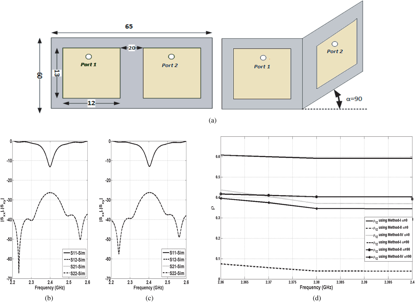
Fig. 5. (a) Two patches with different tilting angle, S-parameters of the two patch antennas, (b)α = 0, (c)α = 90, and (d) the ρ of the two patches.
Fig. 6. S-parameters of the two patch antennas: (a) d = λ/8, (b) d = λ/4, (c) d = λ/2, and (d) the ρ of the two patches.
It is worth mentioning that for well-isolated antennas, the estimation of ρ using method-II will always give low values since the numerator of (5) will be very low and this can lead to wrong values. Increasing the spacing between the elements will decrease ρ since the patterns will be more spatially separated (in a real non-isotropic environment, the values tend to oscillate with distance).
VI. CONCLUSIONS
This work evaluates and discusses the accuracy and complexity of four methods for correlation coefficient (ρ) calculations in MIMO antenna systems. We generalize two of the existing methods (method-III and the parallel equivalent circuit for method-IV) to consider N-antenna elements for the first time. The effect of radiation pattern tilts on the estimation of ρ is the first to be considered in this work. The analysis conducted is applied on three different MIMO antenna systems with various efficiency values. It is found that method-I is the most accurate and should be used all the time. It requires 3D pattern measurements. Method-II is easy to use but fails most of the times to give accurate ρ values even for very efficient MIMO antenna systems because it does not consider the field orientation and tilts. Method-III compensates for some of the large errors encountered by method-II when the efficiency is not high, but starts over estimating the ρ values below certain efficiencies. Thus it should not be used due to its unreliable outcomes. Method-IV provides close estimates compared with method-I only when the antennas are placed in a symmetric way. It fails to give reliable ρ values otherwise. Method-IV requires extra steps for the calculation of the loss factor, thus it is the most complex compared with other methods.
ACKNOWLEDGEMENTS
This work was supported by the deanship of scientific research (DSR) at King Fahd University of Petroleum and Minerals (KFUPM), Dhahran, Saudi Arabia, under project number RG1419.
APPENDIX A
To make method-III valid for N-elements, we provide the steps to generalize it as part of this work contribution. The total radiated field in the far field can be the sum of each element contribution as follows:
 $$\overrightarrow E = \overrightarrow {E_1} + \overrightarrow {E_2} + \cdots + \overrightarrow {E_N}, $$
where the radiated field of element j can be expressed in term of the incident wave a j , M is the constant, which depends on the antenna dimensions and the directivity as well as the wave number k and F j (θ, ϕ) is the far-field pattern using the expression:
 $$\overrightarrow {E_j} = a_j M\overrightarrow {F_j} \left( {\theta, \phi} \right)\displaystyle{{e^{ - ikr}} \over r}.$$
Then the total power can be written as:
 $$P_{tot} = \int \! \int_{allspace} \left \vert {\overrightarrow E} \right \vert ^2 ds.$$
The total power can be also expressed in S-parameter form as:
 $$P_{tot} = a^{\ast} (I - S^{\ast} S)a,$$
where a is the incident wave vector of the N elements, S is N × N scattering matrix and i is the identity vector. The total radiated power from element i with efficiency η rad,i can be as follows:
 $$P_{rad,i} = \left \vert {a_i} \right \vert ^2 \left( {1 - \sum\nolimits_{n = 1}^N {\left \vert {S_{ni}} \right \vert ^2}} \right)\eta _{rad,i}. $$
The total input power from element i can be written as:
 $$P_{in,i} = \left \vert {a_i} \right \vert ^2 \left( {1 - \sum\nolimits_{n = 1}^N {\left \vert {S_{ni}} \right \vert ^2}} \right),$$
Hence, the internal losses power from element i can be written as:
 $$P_{loss,i} = \left \vert {a_i} \right \vert ^2 \left( {1 - \sum\nolimits_{n = 1}^N {\left \vert {S_{ni}} \right \vert ^2}} \right)(1 - \eta _{rad,i} ).$$
If ρ can be related to the power, then the correlation matrix (I − S* S) for different elements i and j can be calculated as in [Reference Blanch, Romeu and Corbella2]. Then ρ can be expressed using orthogonality and power conservation laws as [Reference Hallbjorner4]:
 $$\eqalign{& \left( {\matrix{ {\rho _{11} \left( {1 - \sum\nolimits_{n = 1}^N {\left \vert {S_{n1}} \right \vert ^2}} \right)\eta _{rad,1}} & \cdots & {\rho _{1N} \sqrt {\left( {1 - \sum\nolimits_{n = 1}^N {\left \vert {S_{n1}} \right \vert ^2}} \right)\eta _{rad,1} \left( {1 - \sum\nolimits_{n = 1}^N {\left \vert {S_{nN}} \right \vert ^2}} \right)\eta _{rad,N}}} \cr \vdots & \ddots & \vdots \cr {\rho _{N1} \sqrt {\left( {1 - \sum\nolimits_{n = 1}^N {\left \vert {S_{nN}} \right \vert ^2}} \right)\eta _{rad,N} \left( {1 - \sum\nolimits_{n = 1}^N {\left \vert {S_{n1}} \right \vert ^2}} \right)\eta _{rad,1}}} & \cdots & {\rho _{NN} \left( {1 - \sum\nolimits_{n = 1}^N {\left \vert {S_{nN}} \right \vert ^2}} \right)\eta _{rad,N}} \cr}} \right) \cr & \quad = (I - S^{\ast} S).}$$
However, this equation is with no conduction and dielectric losses. Now, by considering internal losses, the S-parameters matrix can be divided into S-parameters matrix for the ports and another for the radiation function and losses [Reference Hallbjorner4], hence the reflection power losses and the power affects port i due to coupling from port j can be expressed as:
 $${\rho _{loss,ij} = \sqrt {\left( {1 - \sum\nolimits_{n = 1}^N {\left \vert {S_{ni}} \right \vert}^2} \right)(1 - \eta _{rad,i})\left( {1 - \sum\nolimits_{n = 1}^N {\left \vert {S_{nj}} \right \vert}^2} \right)(1 - \eta _{rad,j}} ).}$$
This can be applied for all ports. From the power conservation low:
 $$\eqalign{\sum\nolimits_{n = 1}^N {S_{ni}^{\ast} S_{nj} } & + \rho _{loss,ij} \sqrt {\left( {1 - \sum\nolimits_{n = 1}^N {{\left \vert {S_{ni}} \right \vert}^2} } \right)(1 - \eta _{rad,i})\left( {1 - \sum\nolimits_{n = 1}^N {{\left \vert {S_{nj}} \right \vert}^2} } \right)(1 - \eta _{rad,j}} ) \cr & + \rho _{ij}\sqrt {\left( {1 - \sum\nolimits_{n = 1}^N {{\left \vert {S_{ni}} \right \vert}^2} } \right)\eta _{rad,i}\left( {1 - \sum\nolimits_{n = 1}^N {{\left \vert {S_{nj}} \right \vert}^2} } \right)\eta _{rad,j}} = 0} $$
by solving and considering the worst case for ρ, (6) is obtained.
APPENDIX B
ρ estimation based on the parallel RLC equivalent circuit will have a topology as shown in Fig. 7. V i is the ith element excitation, r loss is the conductance loss, Y rad is the radiation admittance and Z L is the antenna load which is the impedance of the feed cable.

Fig. 7. A lossy network for four-element MIMO antenna as a cascaded parallel equivalent circuit.
The S-parameters between the ports can be measured using a VNA. The lossy part can be considered as a cascaded network with the lossless part as shown in Fig. 7. The S-parameters for the lossy part can be calculated by knowing the values of the conductance impedances. For a four-element MIMO antenna system it is given by (for N-elements, the same procedure is followed):
 $$L_{13} = \left( {\matrix{ {\displaystyle{{r_{1,loss} Z_0} \over {2 + r_{1,loss} Z_0}}} & 0 & {\displaystyle{2 \over {2 + r_{1,loss} Z_0}}} & 0 \cr 0 & {\displaystyle{{r_{3,loss} Z_0} \over {2 + r_{3,loss} Z_0}}} & 0 & {\displaystyle{2 \over {2 + r_{3,loss} Z_0}}} \cr {\displaystyle{2 \over {2 + r_{1,loss} Z_0}}} & 0 & {\displaystyle{{r_{1,loss} Z_0} \over {2 + r_{1,loss} Z_0}}} & 0 \cr 0 & {\displaystyle{2 \over {2 + r_{3,loss} Z_0}}} & 0 & {\displaystyle{{r_{3,loss} Z_0} \over {2 + r_{3,loss} Z_0}}} \cr}} \right),$$
 $$L_{24} = \left( {\matrix{ {\displaystyle{{r_{2,loss} Z_0} \over {2 + r_{2,loss} Z_0}}} & 0 & {\displaystyle{2 \over {2 + r_{2,loss} Z_0}}} & 0 \cr 0 & {\displaystyle{{r_{4,loss} Z_0} \over {2 + r_{4,loss} Z_0}}} & 0 & {\displaystyle{2 \over {2 + r_{4,loss} Z_0}}} \cr {\displaystyle{2 \over {2 + r_{2,loss} Z_0}}} & 0 & {\displaystyle{{r_{2,loss} Z_0} \over {2 + r_{2,loss} Z_0}}} & 0 \cr 0 & {\displaystyle{2 \over {2 + r_{4,loss} Z_0}}} & 0 & {\displaystyle{{r_{4,loss} Z_0} \over {2 + r_{4,loss} Z_0}}} \cr}} \right),$$
where L 13 is the S-parameter matrix of the lossy part in elements 1 and 3 and L 24 is that for elements 2 and 4. It is worth mentioning that in this configuration, identical elements and symmetric placement is considered such that r loss = r 1,loss = r 2,loss = r 3,loss = r 4,loss , and then obviously L 13 = L 24. The Transmission matrix for both S-parameters measured from the VNA and S-parameters for the lossy network part can be calculated from [Reference Frei, Cai and Muller28] to extract the lossless S-parameters as follow:
 $$[S_{lossless} ]_T = [L_{1,3} ]_T [S_{lossy} ]_T^{ - 1} [L_{2,4} ]_T, $$
where [S lossy ] T is the transmission matrix for the S-parameters measured by the VNA, [L i, j ] T is the transmission matrix for the lossy part in element i and element j. To calculate the value of the loss conductance r loss from Fig. 7, the antenna elements can be viewed in two ways; first, it can be defined as four networks with their inactive port connected to the load impedance, so that only port 1 is active. Thus the total efficiency can be calculated as [Reference Stjernman3]:
 $$\eta _{tot1} = \left( {1 - \sum\limits_{j = 1}^4 \left \vert {S_{j1}} \right \vert ^2} \right)\eta _{rad1} \underbrace {\displaystyle{{P_{rad}} \over {P_{rad} + P_{loss}}}} _{},$$
where the underbrace term is the radiation efficiency (η rad ). The relation between V 1 and V j can be calculated from non-excited elements assuming port 1 is excited as (equations for other ports are removed for space constrains but follow same structure):
 $$Y_{21} V^{\prime}_1 + (Y_{22} Z_L + 1)\displaystyle{{V^{\prime}_2} \over {Z_L}} + Y_{23} V^{\prime}_3 + Y_{24} V^{\prime}_4 = 0.$$
By defining k 1j = |V′ j |/|V′1| using the matrix;
 $$\eqalign{&\left( {\matrix{ {k_{12}} \cr {k_{13}} \cr {k_{14}} \cr}} \right) = - \left( {\matrix{ {\displaystyle{1 \over {Z_L}} (Y_{22} Z_L + 1)} & {Y_{23}} & {Y_{24}} \cr {Y_{32}} & {\displaystyle{1 \over {Z_L}} (Y_{33} Z_L + 1)} & {Y_{24}} \cr {Y_{42}} & {Y_{43}} & {\displaystyle{1 \over {Z_L}} (Y_{44} Z_L + 1)} \cr}} \right)^{ - 1} \left( {\matrix{ {Y_{21}} \cr {Y_{31}} \cr {Y_{41}} \cr}} \right).}$$
The radiation efficiencies are calculated from k ij using the following equation:
 $$\eta _{rad1} = \displaystyle{{\sum\nolimits_{j = 1}^4 {k_{1j}^2 Y_{j,rad}}} \over {\sum\nolimits_{j = 1}^4 {k_{1j}^2 Y_{j,rad} +} \sum\nolimits_{j = 1}^4 {k_{1j}^2 r_{j,loss}}}}. $$
In the second way, the antenna system network is defined in such a way that one port is active while all others are terminated with a loss resistance. The total efficiency in that case is found as:
 $$\eta _{tot,1} = \left( {1 - \vert S_{11} \vert ^2} \right) {\displaystyle{{\sum\nolimits_{j = 1}^4 {k_{1j}^2 Y_{j,rad}}} \over {\sum\nolimits_{j = 1}^4 {k_{1j}^2 Y_{j,rad} +} \sum\nolimits_{j = 1}^4 {k_{1j}^2 r_{j,loss} +} \sum\nolimits_{j = 2}^4 {k_{1j}^2 Re(Z_l )}}}} $$
 Mohammad S. Sharawi received the Ph.D. degree in RF systems engineering from Oakland University, Oakland, MI, USA, in 2006. He was a Hardware Design Engineer with Silicon Graphics Inc., Mountain View, CA, USA, from 2002 to 2003. From 2006 to 2008, he became a Faculty Member with the Computer Engineering Department, German Jordanian and Philadelphia Universities in Amman, Jordan. He was a Research Scientist with the Applied Electromagnetics and Wireless Laboratory, Oakland University, from 2008 to 2009 and in 2013. In 2014, he joined the iRadio Laboratory, University of Calgary, Calgary, AB, Canada, as a visiting research Professor until 2015. He is currently a Professor of Electrical Engineering with King Fahd University of Petroleum and Minerals (KFUPM), Dhahran, Saudi Arabia. Dr. Sharawi is the Founder and Director of the Antennas and Microwave Structure Design Laboratory (AMSDL). He is the single author of the book, Printed MIMO Antenna Engineering, Artech House, 2014. He has authored/co-authored seven book chapters in antenna design, MIMO antenna systems and RF systems, along with over 200 refereed international journal and conference paper publications mostly with the IEEE. He holds 12 issued and 14 pending patents from the US-Patent Office. His current research interests include printed multiple-input–multiple-output antenna systems, miniaturized printed antennas and antenna arrays, active integrated antennas, reconfigurable antennas, microwave circuits and electronics, millimeter-wave antennas and antenna arrays, and applied electromagnetics. Dr. Sharawi is an IET Fellow and Senior member of IEEE. He was a recipient of the prestigious Excellence in Scientific Research and Best Research Project Awards from KFUPM in 2015 and 2017. He received conference paper awards in IEEE LAPC 2014, and IEEE MeCAP 2016. He has served/serving on the technical and organizational committees of several international IEEE conferences, especially EuCAP, APS, APWC, APCAP, and ICCE.
Abdelmonim T. Hassan is currently pursuing his Ph.D. degree in Electrical Engineering at Concordia University, Canada. He did his M.Sc. degree under the supervision of Professor M. S. Sharawi at KFUPM, Saudi Arabia. His research interests are printed MIMO antenna systems and mobile communications.
 Muhammad U. Khan received the B.S. degree in Electrical Engineering from the National University of Sciences and Technology (NUST), Pakistan, in 2006 and the M.S. degree in Electrical Engineering from the GIK Institute of Engineering Sciences and Technology, Pakistan, in 2008. He received his Ph.D. in Electrical Engineering from King Fahd University of Petroleum and Minerals (KFUPM), Dhahran, Saudi Arabia, in 2014. He is currently an Assistant Professor at the National University of Science and Technology (NUST), Islamabad, Pakistan. His current research interests include miniaturization of printed antennas, MIMO antennas, and metamaterial antennas.


