I. INTRODUCTION
Modernization of global navigation satellite system (GNSS) receivers in aviation, maritime traffic, or consumer electronics envisage accurate and robust information of the position, velocity, and time in all interference situations and environments. Therefore, in addition to improved precision due to the use of broader bandwidth and dual-band operation, sophisticated null-steering algorithms for interference cancellation, and multi-path mitigation are foreseen to achieve maximum robustness in navigation signal reception and processing. In practice, this visualizes the deployment of a multi-element receiver. One example of a state-of-the-art GNSS four-element antenna array receiver is the GALANT demonstrator developed at the German Aerospace Center (DLR) in order to achieve robust navigation for safety-of-life applications [Reference Heckler, Cuntz, Konovaltsev, Greda and Meurer1]. Its overall antenna array size is approximately 30 cm × 30 cm, essentially due to a large inter-element separation. In the past reported robust GNSS antenna arrays' inter-element separation has always been half of the free-space wavelength [Reference Ly2–Reference De Lorenzo, Rife, Enge and Akos4].
Antenna arrays are typically designed with a large inter-element separation in order to avoid mutual coupling. An optimal choice for the inter-element separation is typically half of the free-space wavelength, where the mutual coupling is minimal. However, at the L1 band (1575.42 MHz), this is approximately 10 cm, which makes the overall antenna size significantly bulky. This large inter-element separation results in certain space, weight, and cost constraints, which limit the utilization of multi-element antenna receivers in modern applications, e.g., mobile or hand-held consumer electronics. Reducing the inter-element separation certainly leads to a compact antenna array design, but then it is impregnated with the strong mutual coupling between the single elements, which degrades the radiation and beamforming performance significantly.
Concerning the compact arrays, a suitable choice of the antenna array having a specific number of elements and inter-element separation is necessary to determine for any particular application or scenario. Moreover, the mutual coupling in the antenna array can be alleviated using a decoupling and matching network (DMN) based on the eigenmode-excitation principle [Reference Irteza, Murtaza, Caizzone, Stephan and Hein5, Reference Volmer6]. These modes are orthogonal in nature and, therefore, perfectly decouple the network ports. With respect to this approach, the exploitation of high-order modes is vital for the multi-path and interference mitigation [Reference Basta7], this holds also true for the conventional half-wavelength antenna arrays. Generally, this DMN is considered lossless in the literature when analyzing the performance gain of the antenna array. This approach overlooks the losses and the noise contribution of the DMN, which may play a limiting role in noise-limited navigation receivers. Therefore, a realistic consideration of dissipation losses is indispensable for the analyses.
For navigation applications, the available satellite carrier-to-interference-plus-noise ratio (CINR) directly defines its acquisition and tracking capability. Therefore, the construction of a realistic receiver model including the noise characteristics of the environment, the antenna array, and the front-end is vital in order to derive the equivalent CINR as a figure-of-merit for compact arrays, especially when impinged with arbitrarily polarized interferers. In this work, we use the equivalent CINR at the input of first-stage amplifier for different interference scenarios. Since interferers can be right-hand-circularly polarized (RHCP), left-hand-circularly polarized (LHCP), or linearly polarized (LP), it is important to determine the influence of the polarization impurity of the compact array in the higher-order modes on the navigation accuracy.
In Section II, we derive the theoretical background needed to understand the performance of compact navigation antenna arrays. In Section III, we present our chosen antenna array design and the DMN, as well as measured radiation performance. In Section IV, robustness of the compact receiver in an interference-limited scenario is investigated by computing the equivalent CINR. In Section V, the complete four-element GNSS antenna array receiver is described, and measurements in a real interference scenario for the jammer-to-signal ratios (JSRs) are carried out, in order to verify the results obtained in the preceding section.
II. COMPACT ANTENNA ARRAYS
For the evaluation of the antenna array, it is necessary to model and analyze the effects of power dissipated within the antenna and reflected due to the impedance mismatch along with power radiated in the presence of coupling between the neighboring elements. Generally, the losses within the antenna are associated with the dielectric substrate materials and the finite conductivity of the metal surfaces. Therefore, especially for printed antennas, their practical characterization is crucial for the realistic analysis. In addition, the compact antenna array configurations inherit finite real-parts of the mutual impedances Z ij, which result in feed-impedances for the individual radiators different from their self-impedances depending on the directions-of-arrival, giving rising to active reflection [Reference Balanis8]. All of these effects adversely affect the total efficiency of the antenna array.
In terms of the compact array, our main objective is to initially formulate an algorithm for obtaining its radiation matrix H, and then determine the realized radiation efficiencies including all of the aforementioned losses. In [Reference Balanis8], Volmer et al. have presented a technique for deriving this matrix using the scattering matrix S and assuming a lossless antenna array
 $$P_{acc} = P_{in} - P_{re} = {\bf a}^H {\bf a} - {\bf b}^H {\bf b} = {\bf a}^H \lpar {\bf I} - {\bf S}^H {\bf S}\rpar {\bf a} .$$
The total incident power P in is expressed using the antenna excitation vector a, whereas the total reflected power P re is represented by the antenna reflection vector b. The mutual coupling between the radiating elements means that the non-diagonal elements are non-zero. Therefore, the reflected wave vector is related to the excitation vector by b = Sa, which results in the radiation matrix of the antenna array as:
 $${\bf H}_{acc} = {\bf I} - {\bf S}^H {\bf S} .$$
Here, the subscript refers to the accepted power by the antenna array. In case of ideally lossless antenna, this is equivalent to the radiated power. However, a practical solution, including the losses of the antenna, can be derived using the complex-valued realized-gain amplitude patterns of the antenna array relative to an isotropic radiators f (θ, ϕ) (each column represents the individual radiator), for determining the radiation matrix:
 $$\eqalign{{\bf H}_{rad\theta } & = \displaystyle{1 \over {4\pi }}\vint {{\bf f}_\theta \lpar \theta\comma \; \phi \rpar ^H \cdot {\bf f}_\theta \lpar \theta\comma \; \phi \rpar } \, d\Omega\comma \; \cr {\bf H}_{rad\phi } & = \displaystyle{1 \over {4\pi }}\vint {{\bf f}_\phi \lpar \theta\comma \; \phi \rpar ^H \cdot {\bf f}_\phi \lpar \theta\comma \; \phi \rpar \, } d\Omega\comma \; \cr {\bf H}_{rad}& = {\bf H}_{rad\theta } + {\bf H}_{rad\phi } .} $$
The subscript “rad” indicates the radiated power. It may be noted for the case of a lossless array that Hrad = Hacc.
A) Eigenanalysis
The radiation matrix H is a real-valued symmetric matrix. Therefore, it is diagonalizable by orthogonal matrices. One such method is the eigendecomposition (or spectral decomposition) of the radiation matrix into the respective eigenvectors and eigenvalues. These eigenvectors are orthogonal in nature and thus represent the excitation vectors for a multi-element antenna array resulting in decoupled ports [Reference Volmer, Weber, Stephan, Blau and Hein9]:
 $${\bf H} = {\bf Q\Lambda Q}^H\comma \; $$
 $${\rm where}\; {\bf \Lambda } = {\rm diag}\lcub \lambda _1\comma \; \lambda _2\comma \; \ldots\comma \; \lambda _n \rcub .$$
The columns of Q represent the respective eigenvectors, which produce orthogonal patterns, containing all degrees-of-freedom of the antenna array. The corresponding eigenvalues λ i for each eigenvector times 100 represent the eigenefficiency (or radiation efficiency), i.e., the relative power of the respective eigenvector or the eigenmode actually radiated into the far-field [Reference Chaloupka, Wang and Coetzee10]. The worst-case eigenefficiency is always the radiation efficiency for the highest-order mode, given by the λ min = min {λi}.
B) Equivalent CINR
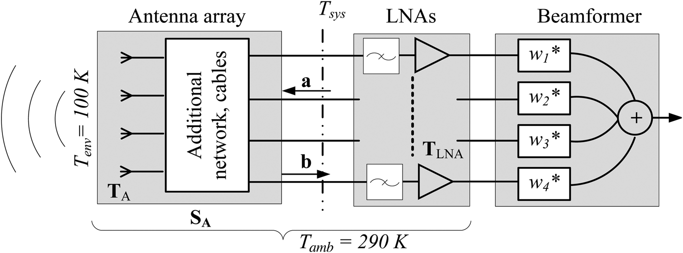
In a navigation receiver, it is important to characterize further the performance of the compact antenna array in terms of the CINR. The higher the CINR the better is the navigation accuracy of the system. The considered receiver model to calculate the CINR is illustrated in Fig. 1. Here, SA indicates the scattering matrix of the antenna array integrated with additional components connected between the front end and the antenna array. TA and TLNA represent the noise correlation matrices of the antenna array and the low-noise amplifiers, respectively. The equivalent CINR is calculated after applying the null-steering algorithm, described in Section IV; the weights are indicated by w i. Non-linear effects due to analog-to-digital conversion are not considered in this model. Therefore, the equivalent CINR for the receiver is
 $$CINR\lpar \phi\comma \; \theta \rpar = \displaystyle{{C\lpar \phi\comma \; \theta \rpar } \over {\sum\limits_{i = no.\, \, of\, \, interferers} {I\lpar \phi _i\comma \; \theta _i \rpar } + N_o }}.$$
Fig. 1. Receiver model.
Here, the equivalent available carrier power is calculated from:
 $$C\lpar \phi\comma \; \theta \rpar = C_{sat} {\bf w}^H {\bf f}_{RHCP} \lpar \phi\comma \; \theta \rpar {\bf f}_{RHCP}^H \lpar \phi\comma \; \theta \rpar {\bf w}\comma \; $$
where C sat is the power received by an ideal RHCP isotropic antenna, and w is the vector of the weighting coefficients in the null-steering algorithm. The individual elements of the column vector fRHCP (ϕ, θ) are derived from the Ludwig transformation of fθ(ϕ, θ) and fϕ(ϕ, θ) [Reference Balanis8].
The noise power spectral density is derived from the equivalent system noise temperature T sys, referred to the LNA inputs:
 $$N_o = k_B T_{sys} = k_B \underbrace {{\bf w}^H {\bf T}_A {\bf w}}_{T_A } \;+\; k_B \underbrace {\displaystyle{{{\bf w}^H {\bf T}_{LNA} {\bf w}} \over {{\bf w}^H \left({{\bf I} - {\bf S}_A {\bf S}_A^H } \right){\bf w}}}}_{T_{LNA} }.$$
The combined noise–temperature correlation matrix of the antenna array is calculated using the measured radiation matrix given in equation (3) and the scattering matrix of the antenna array. The antenna–temperature correlation matrix TA using the radiation matrix and scattering parameters of the antenna array is given as:
 $${\bf T}_A = T_{env} {\bf H}_A^T + T_{amb} \left({\left({{\bf I} - {\bf S}_A {\bf S}_A^H } \right)- {\bf H}_A } \right)^T .$$
TA includes noise received from the environment as well as from the antenna array and connected cable or network; T env = 100 K is the assumed equivalent isotropic environmental temperature for GNSS conditions [11]; T amb = 290 K is the ambient temperature of the antennas. I denotes the identity matrix.
The noise contribution from the amplifiers is calculated according to [Reference Engberg and Larsen12, Reference Irteza13]. The equivalent noise–temperature correlation matrix is defined as:
 $${\bf T}_{LNA} = \left({{\bf T}_\alpha + {\bf S}_A {\bf T}_\beta {\bf S}_A^H \left. { - {\bf S}_A {\bf T}_\gamma - {\bf T}_\gamma ^H {\bf S}_A^H } \right)} \right.\comma \; $$
where we assume that the noise generated by every single LNA is uncorrelated with all other amplifiers. Therefore, the input-referred noise correlation matrices in equation (10) simplify to Tα = T αI, Tβ = T βI, and Tγ = T γI, in which T α, T β, and T γ are calculated from the measured noise parameters minimum noise figure F min, equivalent noise resistance R n, and optimum noise impedance Z opt as discussed in [11].
The equivalent available interference power is defined as [Reference Irteza14, Reference Irteza15]:
 $$I\lpar \phi\comma \; \theta \rpar = P_{int} {\bf w}^H {\bf f}_{CP} \lpar \phi\comma \; \theta \rpar {\bf f}_{CP}^H \lpar \phi\comma \; \theta \rpar {\bf w}$$
for a circular polarized (CP) interferer, i.e., RHCP or LHCP,
 $$\eqalign{I\lpar \phi\comma \; \theta \rpar = \displaystyle{1 \over 2}P_{{int}} \left({{\bf w}^H {\bf f}_{RHCP} \lpar \phi\comma \; \theta \rpar {\bf f}_{RHCP}^H \lpar \phi\comma \; \theta \rpar {\bf w}} \right. &\cr \left. { + {\bf w}^H {\bf f}_{LHCP} \lpar \phi\comma \; \theta \rpar {\bf f}_{LHCP}^H \lpar \phi\comma \; \theta \rpar {\bf w}} \right)\comma \; &} $$
for an LP interferer. P int is the power received from the interferer by an ideal co-polarized isotropic antenna.
III. DECOUPLED AND MATCHED COMPACT ANTENNA ARRAY
A) Optimal antenna array
Using the eigenanalysis, the optimal configuration for the coupled navigation antenna array can be determined, which depends on the choice of number of elements, inter-element separation, and the geometry. As mentioned earlier, in any compact array the highest-order mode's radiation efficiency, represented by the minimum eigenefficiency, is affected the most by mutual coupling. Therefore, optimizing the array configurations to improve the minimum eigenefficiency will alleviate the detection and tracking capability of the receiver especially if jammed by the maximum tolerable number of interferers [Reference Irteza, Murtaza, Caizzone, Stephan and Hein5].
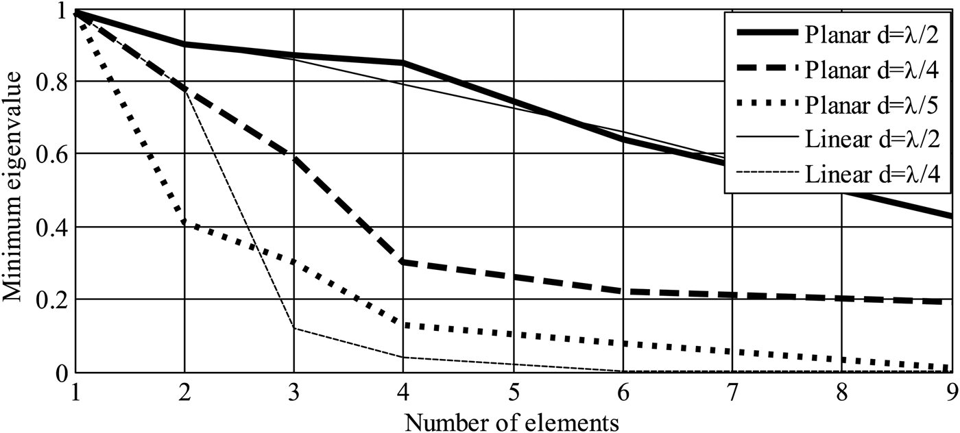
Different linear (1D) and planar (2D) array configurations, not particularly square shape, with different numbers of elements were modeled and simulated in CST Microwave Studio [Reference Van Trees16]. These arrays were optimized with respect to inter-element separations and geometry configurations for maximum values of the minimum eigenefficiencies. Different geometries for 3, 4, 6, and 9 elements were designed with inter-element separations d as shown in Fig. 2. The individual radiating element is a square printed patch antenna, assumed lossless for these simulations. It can be seen that for increasing number of elements the minimum eigenefficiency reduces significantly for compact arrangement; this holds also true for the conventional half free-space wavelength antenna array. On the other hand, for a given number of elements, e.g., four elements, efficiency drops to 15% with d = λ/5 from 30% with d = λ/4 for a planar array. It can be generalized that the planar geometrical configuration alleviates the effect of mutual coupling and improves the efficiency performance of the highest-order mode.
Fig. 2. Minimum eigenvalues for lossless arrays versus number of radiating elements, for different inter-element separations and geometrical arrangements.
In order to achieve 20% minimum eigenefficiency and considering 50% losses within the antenna material, the appropriate array configuration is a four-element antenna with inter-element separation of a quarter of the free-space wavelength and a square shaped geometry. Apparently, the number of nulls, i.e., number of interferers that can be cancelled simultaneously, is then limited to three, with one degree-of-freedom dedicated to the desired satellite direction. In the following sections, the discussion is limited to a four-element square-shaped antenna array with an inter-element separation of d = λ/4. For any other application, the suitable array configuration may be different, depending on the requirements of the number of interferer cancellations, the signal bandwidth, and the receiver sensitivity.
B) Decoupling and matching
Besides the low radiation resistance of the higher-order modes, the reduction in the radiation efficiency of the higher-order modes of the compact antenna arrays is mainly associated with the reflection and dissipation power losses. The dissipation losses cannot be recovered. However, the reflection losses caused by the mutual coupling can be recuperated primarily by decoupling the antenna elements. Once decoupled, the antenna elements are independently matched in order to transfer the entire available power between the antenna and receiver. The techniques to decouple of the antenna elements are divided into two major categories:
1. Element-level decoupling: Electromagnetic band-gap structures or parasitic elements in between the radiating elements. This technique suffers from the narrow-band characteristics of the additional structures.
2. Circuit-level decoupling: Hybrid-couplers or the lumped components. This technique suffers from additional dissipation losses.
In this paper, we limit our discussion to circuit-level DMN. We consider the implementation using 180°-hybrid couplers. We are mainly concerned with the benefits of such a DMN for compact antenna arrays designed for navigation applications.
C) Antenna array integrated with DMN
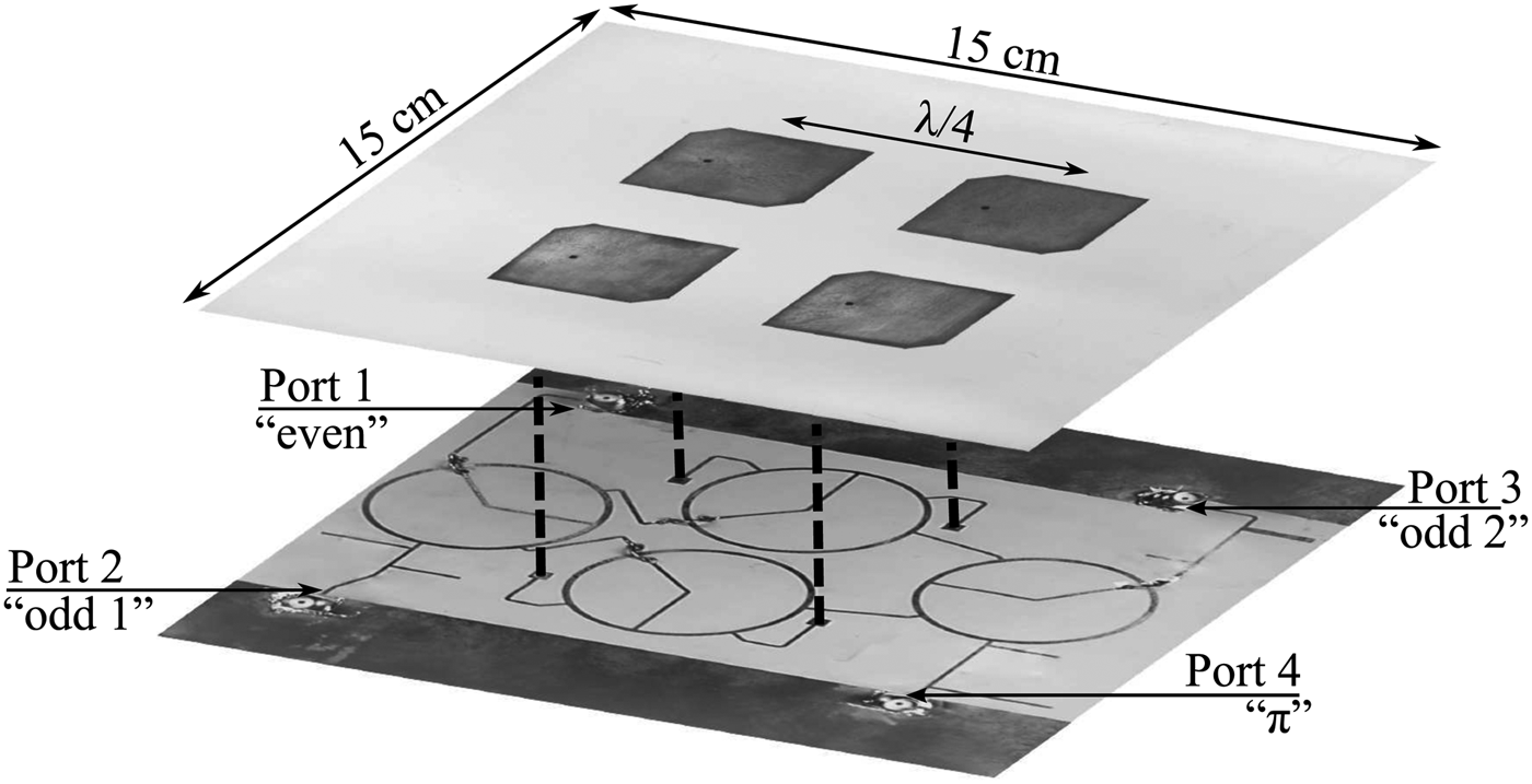
The antenna array integrated with the DMN is shown in Fig. 3. The antenna array comprises four truncated square patches, with an inter-element separation of one quarter of the free-space wavelength, as shown in Fig. 2. The substrate has a relative dielectric permittivity of ε r = 10.2, and a thickness of 2.74 mm. The truncated square patches typically exhibit narrow input impedance matching and axial-ratio bandwidth [Reference Balanis8], which is enhanced by properly adjusting the thickness of the substrate to this value. The 10-dB matching bandwidth measured for the antenna array at the desired frequency, centered at 1575.42 MHz amounts to 4 MHz and a fractional bandwidth of 0.3%. However, the measured mutual coupling coefficients exceed −10 dB, reaching a maximum of −8 dB. This causes the feed impedance of the antenna elements to vary for different directions-of-arrival, especially in the presence of nulls, which means reduced available carrier power due to mismatch power loss.
Fig. 3. Top: Antenna array. Bottom: Decoupling and matching network indicating the respective mode excitations, bottom view of the integrated antenna array and DMN.
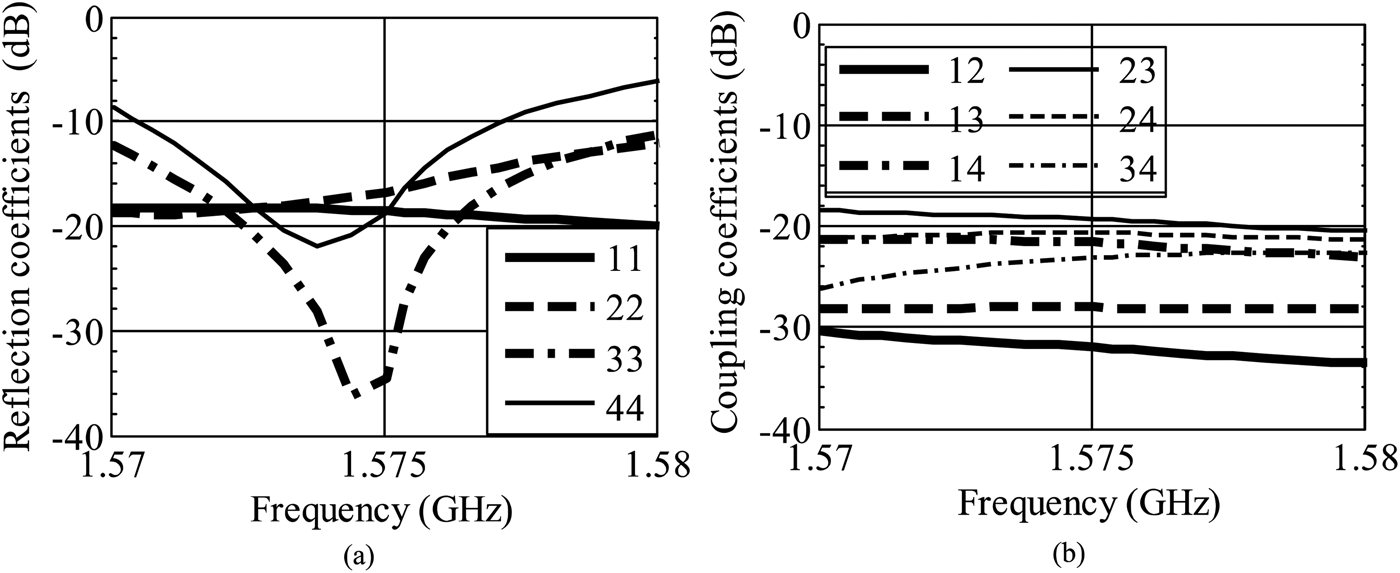
As the antenna array is symmetric, its eigenvectors correspond to the excitation vectors formed at the output of four 180°-hybrid couplers if connected as shown in Fig. 3. In addition to the decoupling of the antenna elements, tuning stubs provide matching of the individual modes. The DMN is designed using a dielectric substrate with relative dielectric permittivity of ε r = 3.55 and a thickness of 0.25 mm. In order to minimize the losses between the network and the antenna feed-points, the outputs of the DMN are directly connected to the radiating elements using metalized vias. The measured reflection coefficients S ii are below −10 dB for all modes, as shown in Fig. 4(a). The coupling coefficients S ij are below −17 dB, as shown in Fig. 4(b).
Fig. 4. Measured scattering parameters of the antenna array with DMN. (a) Measured modal input reflection coefficients S ii. (b) Coupling coefficients S ij.
It is worth mentioning that the 10-dB matching bandwidth of the π-mode is quite narrow, as compared with the other modes. Therefore, application-specific bandwidth requirements for the antenna array also decide the choice of count and mutual separation of the antenna elements.
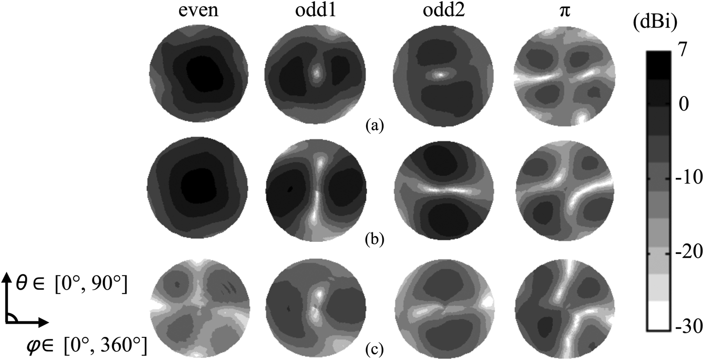
D) Co-polarization
The antenna array is optimized for RHCP co-polarization. The corresponding measured RHCP modal radiation patterns of the compact antenna array without DMN are shown in Fig. 5(a). With DMN, the modal RHCP radiation patterns are displayed in Fig. 5(b). The even mode, with and without DMN, displays a maximum realized gain of 6 dBi. In contrast, the π-mode has a maximum gain of −2.6 dBi and −5 dBi with and without DMN, respectively.
Fig. 5. Realized-gain radiation patterns of the compact array (polar gray-coded maps). (a) Ideal eigenmodes for the array excited with the exact eigenvectors with RHCP. (b) Measured (RHCP) at the respective output ports of the DMN for the L1 frequency. (c) Measured (LHCP) patterns with DMN.
E) Cross-polarization
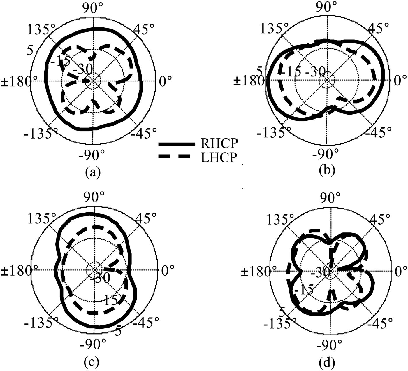
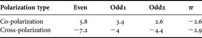
For the array with DMN, the cross-polarization realized gains of the higher-order modes are analogous to those for the co-polarization, except for the even-mode, as shown in Fig. 5(c). This may degrade the radiation performance of the antenna array under the influence of interferers. Also, the measured RHCP and LHCP gain ϕ-cut is shown in Fig. 6, for all modes at a respective elevation of θ = 75°. The even-mode gain is uniform over the azimuth with no nulls. However, the π-mode possesses the maximum number of nulls (three in our case) with a depth up to −40 dBi. It can be noted that at the null location of the co-polarization, particularly for the π-mode, the cross-polarization gain is up to −4 dBi. In addition, the nulls are not distinct at this low-elevation angle. In Table 1, the maximum realized gains for both polarizations are summarized. The maximum cross-polarization realized-gain for the even and the π-mode is −7 and −2.9 dBi, respectively.
Fig. 6. Measured realized-gain co-polarization (RHCP) and cross-polarization (LHCP) modal radiation patterns (ϕ-cuts) at θ = 75° in dBi for (a) the even mode, (b) the odd1 mode, (c) the odd2 mode, and (d) the π mode.
Table 1. Measured maximum modal realized gains with DMN in dBi.
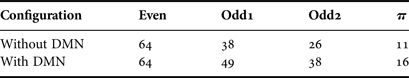
The total modal eigenefficiences are shown in Table 2, which are obtained using the measured realized-gain amplitude patterns in equations (3)–(5). It can be seen that with DMN the antenna array radiation efficiencies are significantly improved for all modes except the even mode.
Table 2. Measured total modal eigenefficiencies in %.
IV. ROBUSTNESS OF THE RECEIVER
In order to derive the CINR, C sat is considered to be −157 dBW [11]. Then, the desired signal direction-of-arrival (DoA) is steered across the upper hemisphere, while the directions-of-interference (ϕ i, θ i) are kept fixed. Each weighting-coefficient vector w for every DoA is applied to equations (7)–(10), and the CINR are calculated for the respective DoA using equation (6). We assume that the interferers impinge from low-elevation angles, i.e., θ i = 75°, because the high-elevation interferers are unlikely to become relevant in realityFootnote 1. Therefore, in low-elevation angles the performance comparison of the antenna array with and without DMN is not significantly affected by the choice of incident angle. Furthermore, due to numerical limitation in case of the conventional null-constraint beamformer, the weights are zero for the similar direction of source and interference; the equivalent CINR cannot be calculated for the directions-of-interference. We consider scenarios with different numbers of arbitrarily polarized interferers for the evaluation of the antenna array. In these scenarios, the equivalent received power of each interferer is set to −117 dBW, which is 40 dB higher than the signal power.
The front-end comprises four independent low-noise amplifiers, each with a low-loss filter in front for better out-of-band interference rejection. The measured on-board noise parameters of the front-end channels are F min = 1.66 dB, R n = 8.2 Ω, and |Z opt| = 29 Ω [Reference Engberg and Larsen12]. We assume that the noise contributions from other components are negligible and, therefore, neglected in these measurements.
To assess the equivalent CINR, a modified version of the well-known null-constraint beamformer [17], differing in the selection of the zero-order constraints, is considered. The optimum weighting coefficients are obtained using:
 $${\bf w} = {\bf w}_d^H\; - \lpar {\bf w}_d^H {\bf w}_I \lpar {\bf w}_I^H {\bf w}_I\rpar ^{-1} {\bf w}_I^H \rpar \comma \; $$
where wd is the steering vector response in the desired direction of the signal, wI is defined as the null-constraint matrix for the unwanted direction of interferers, with the columns representing the interferers.
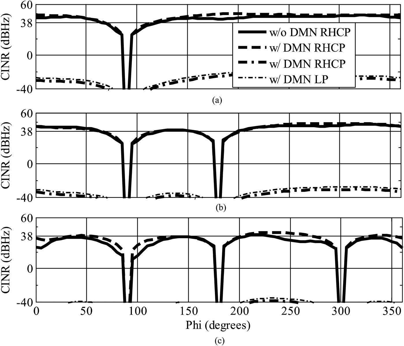
A) Single interferer
One interferer, RHCP, LHCP, or LP, fixed at ϕ i = 90°, θ i = 75° is superimposed by the GNSS signal. The resulting CINR ϕ-cuts for all three polarizations with and without DMN are shown in Fig. 7(a). It can be observed that the impact of the DMN in terms of CINR, while considering RHCP interferer, is marginal. However, with DMN, since nulling and desired-direction constraints are calculated with respect to RHCP only, the null-steering clearly leads to CINR values higher than the optimal acquisition limit of 38 dBHz only for a single RHCP interferer, whereas a LHCP or a LP interferer degrades the performance. Here, the maximum CINR drops below 0 dB, which is almost 75 dB below the RHCP case.
Fig. 7. ϕ-cut at θ = 75° for the calculated CINR in dBHz with and without DMN (a) for one interferer, (b) two interferers, and (c) three interferers.
B) Two interferers
In the second scenario, we study the illumination with two interferers, fixed at ϕ i= 90° and 180°, θ i= 75°. It can be observed in Fig. 7(b) that there is no advantage with DMN, and the CINR in case of the RHCP interferer is greater than 38 dBHz with and without DMN. The maximum CINR in this radiation plane is slightly lowered by 1 dB compared to a single RHCP interferer, which is fully acceptable. Again, for LHCP or LP interferers, the CINR in the desired directions drops well below 0 dBHz, due to high cross-polarization content of the high-order modes.
C) Three interferers
The maximum number of interferers that can be mitigated using a four-element antenna array is three, with one degree-of-freedom used for each desired direction [Reference Irteza15]. This is the worst case since it entirely relies on the exploitation of the π-mode, which is most strongly affected by mutual coupling. Therefore, with three interferers fixed at ϕ i= 90°, 180°, and 300°, θ i = 75° directions, the CINR shown in Fig. 7(c) clearly indicates the superior performance if a DMN is employed. The CINR increases by at least 3 dB in all directions with DMN, and a maximum increase of as much as 8 dB in some directions, which is quite significant for navigation signals.
D) Maximum degrees-of-freedom for nulling
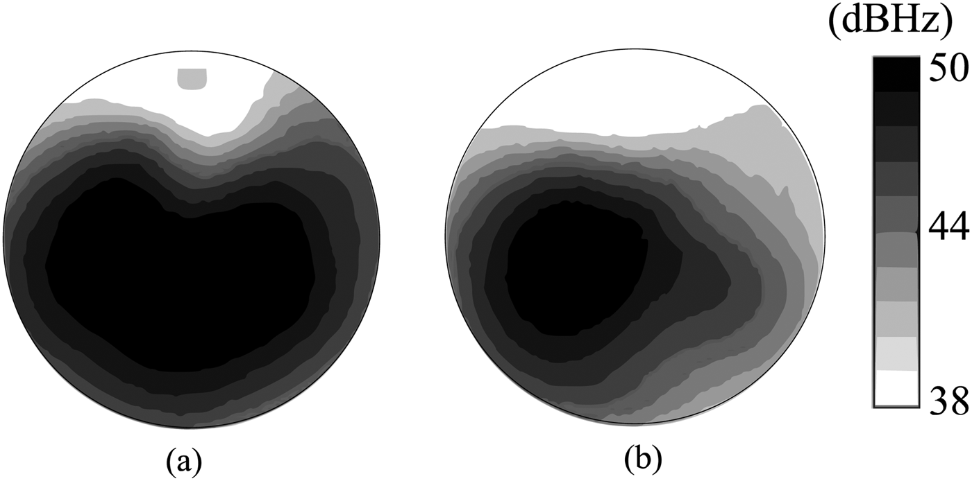
If we use an additional LHCP null-constraint in the previously considered single-LP interferer situation, we fix one of the remaining two degrees-of-freedom for the suppression in cross-polarization. If the RHCP and LHCP constraints are nulling the same DoA, LP interferes can be completely mitigated. With this configuration, we achieve a similar CINR performance in all azimuth directions as compared to a single RHCP interferer.
The CINR patterns calculated for a RHCP or LP interferer, fixed at ϕ i = 90°, θ i = 75° are shown in Fig. 8. Since there is still one degree-of-freedom available, another co-polarized null-constraint can be incorporated. For our four-element circularly polarized compact antenna array, this approach of interference cancellation will ensure nulling of, at maximum, one arbitrarily polarized interferer and either one RHCP or one LHCP interferer [Reference Irteza15].
Fig. 8. Computed CINR in dBHz for one interferer, applying a multiple-constraint beamforming algorithm. (a) RHCP interferer (upper-hemisphere) and (b) LP interferer (upper-hemisphere).
V. FOUR-ELEMENT GNSS ANTENNA ARRAY RECEIVER
Within the framework of the public-funded project KOMPASSION, a complete GNSS demonstrator called KOMPASSION, shown in Fig. 9, was developed which comprises the compact antenna array, a miniaturized multi-channel analog front end, and a digital receiver. It is a novel attempt to verify the functionality of compact arrays for navigation applications and to evaluate the benefit of the DMN in interference-limited scenarios. The demonstrator tests and measurements were carried out at the designated European facility Galileo Test Range (GATE) in Berchtesgaden, Germany [18]. This facility is capable of providing artificial Galileo satellite (pseudolite) signals, which are required due to incomplete coverage of Galileo satellites in the space during the time of the measurement of the demonstrator shown in Fig. 10. In GATE, it is also permitted to transmit high-power GNSS interference signals, which are otherwise prohibited throughout Europe.
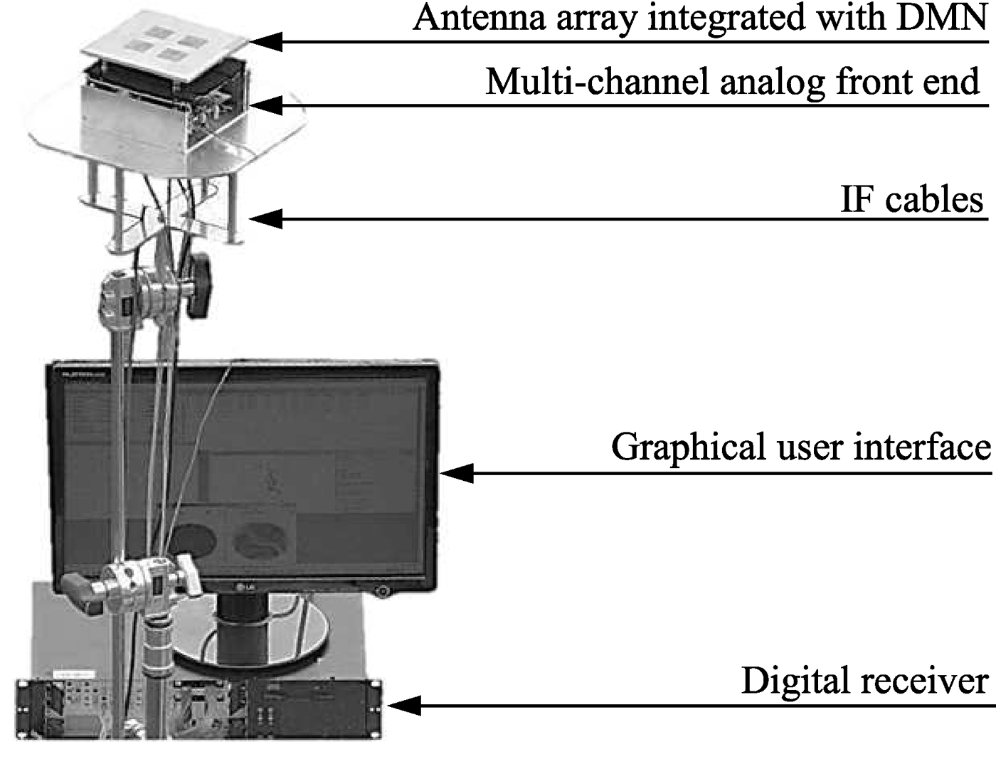
Fig. 9. GNSS four-element compact antenna receiver demonstrator.
Fig. 10. A test-setup against interference of the KOMPASSION demonstrator at Galileo Test Range (GATE) in Berchtesgaden, Germany.
A) Static test-setup
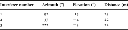
The setup comprised three antennas connected to variable power continuous sinusoidal wave sources. The interferer 1, shown in Fig. 10, transmit frequency was set to GPS center frequency. The interferers 2 and 3 had a frequency offset of ±100 kHz to avoid the superposition of the interference signals at the receiver. During the testing of the receiver the power and the number of interferers were varied to investigate the performance parameters while keeping the geometry constant. The geometrical configuration details of the interferer positions are given in Table 3. The received jammer power was recorded at the receiver's position using reference antenna measurements, which had an accuracy of ±3 dB approximately.
Table 3. Geometrical configuration of the interferers.

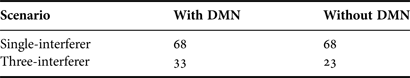
B) Jammer-to-signal ratio
In Table 4, the measured maximum JSR for high elevation satellites is shown in the case of one interferer and three interferers, while keeping a CINR at a threshold of 38 dBHz. As it was calculated analytically that with one interferer there is no advantage of the DMN, similarly, here it was recorded that the JSR is the same with and without DMN. We observed previously that in order to maximize the robustness, i.e., to achieve higher JSR, especially in the three-interferer scenario, it is necessary to employ a DMN. This theoretical outcome was validated by our measurements, which are demonstrating an approximately 10 dB higher JSR with DMN as compared to without DMN for the same antenna array. The imprecision in the JSR difference is due to a jammer-power step size of 5 dB that was required in order to optimize the test time. Future measurement campaigns are currently under preparation in which smaller step sizes will guarantee results that are more accurate. Nevertheless, the antenna array with DMN is capable of coping with stronger jammer power than without DMN. Obviously, these absolute JSR values are not valid for all situations, while the influence of the interferers' position and available satellite constellation is not considered. In addition, the effects of arbitrarily polarized interferers could not yet been recorded due to the limited measurement time, but are planned for the future.
Table 4. Maximum allowed JSR (dB) to keep the CINR above 38 dBHz measured at GATE, all interferers transmit CW signal.
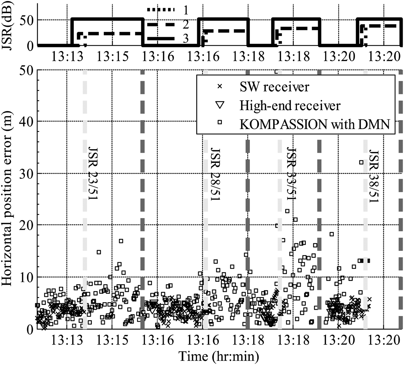
In the end, maintaining the same positions of the interferers as mentioned in Table 3 and replacing the source of the third interferer with a commercial personal privacy device that transmits a sweeping CW signal within the GPS band [Reference Pullen and Gao19], horizontal position errors were recorded. In comparison, two different types of commercial single-element GPS receivers were also investigated. The standard receiver (SW receiver) had no anti-jamming capability, whereas high-end receiver provided anti-jamming capability against CW interferers. In Fig. 11, the horizontal position error for the three receivers is plotted. It can be seen that the commercial receivers completely loose the position information when the three interferers are switched on; however, the developed four-element compact antenna array navigation receiver is able to mitigate the interferers until JSR of 33 dB. Therefore, additional spatial nulling of the interference provides superior positioning performance in regards to robustness, which is critical for safety-of-life applications in the navigation receivers.
Fig. 11. Top: JSR measured at the position of device under test for different interferers independently in dB, interferer number 1 has a fixed JSR of 51 dB. Bottom: Measured horizontal position error by the test receivers, in meters.
VI. CONCLUSIONS
We presented a robust satellite navigation receiver based on a four-element compact planar antenna array using a DMN. Firstly, we presented a method to determine the optimal configuration of the compact antenna arrays by maximizing the worst-case radiation efficiency. Then, the navigation receiver's equivalent CINR was derived in order to analyze the performance of the antenna array with and without DMN when impinged with arbitrarily polarized interferers. It is revealed that the DMN improves the CINR performance of the antenna array with a maximum number of co-polarized interferers by at least 3 dB in all directions, and up to a maximum of 10 dB in certain directions. However, it is observed that the elevated cross-polarization content for the higher-order modes, resulting from the mutual coupling between the antenna elements, requires extra degrees-of-freedom to suppress partly or fully cross-polarized interferers. The receiver, in the case of the chosen null-steering technique, is capable of mitigating either one LP and one CP interferer or three CP interferers. Here the question arises how many nulls are adequate in realistic multi-path and interference scenarios. For compact arrays, a further increased number of antenna elements, covering the same aperture area, lead to inefficient degrees-of-freedom, narrow bandwidth, and reduced CINR because of the increased mutual coupling. Therefore, a trade-off between the number of elements and the compactness of the array has to meet a certain CINR threshold, especially for GNSS applications, while encountering a specific number of arbitrarily polarized interferers. Finally, measured performance data of the compact antenna array GNSS demonstrator were presented. The measured compact antenna array receiver's JSR confirms the superior performance of the antenna array with DMN for the three-interferer case. For a single interferer, the ration remains unchanged with and without DMN. However, for a CINR above 38 dBHz, the JSR is reduced by approximately 10 dB without DMN. This validates the necessity of the DMN in compact navigation antenna arrays particularly limited by interference. These results also lay the foundation for the penetration of satellite navigation into a multitude of advanced applications where robustness forms a prerequisite.
ACKNOWLEDGEMENTS
We gratefully acknowledge valuable contributions from our project partners at RWTH Aachen and at the Institute for Communication and Navigation at DLR Oberpfaffenhoffen, especially Professor Dr. M. Meurer, and Dr. A. Dreher, for their valuable suggestions and discussions during this work. We express our great appreciation to Dr. C. Volmer at Ilmenau University of Technology for his constructive suggestions during the planning and development of this work. The authors would also like to thank M. Huhn and M. Zocher for their technical assistance. This work has been supported by the German Aerospace Center (DLR) on behalf of the German Federal Ministry of Economics and Technology under grant nos 50 NA 1007 and 50 NA 1405.
 S. Irteza was born in 1983 and did his Bachelors in Electronics Engineering from Ghullam Ishaq Khan Institute (GIKI) of Technology in 2004. Soon after graduating, he joined Pakistan's research organization NESCOM, in the Department of Radars and Communications as an Assistant Manager. His area of work mainly related to the development of Ku-Band monopulse radar RF front end. Then, in 2006, he did his Masters in Wireless Systems at KTH Sweden with full scholarship from National University of Sciences and Technology (NUST), Pakistan. He returned to NUST after completing his Master studies, and joined as a Lecturer in the College of Telecommunications Engineering. Since 2010, he has been a Ph.D. candidate at the Department of RF and Microwaves at Ilmenau University of Technology, Germany. His research interests include antenna designing, RF front end development, compact antenna arrays, microwave devices, estimation, detection, and modulation in wireless systems particularly in GNSS.
E. Schäfer (S'10) received his B.Sc. and M.Sc. degrees in Electrical Engineering and Information Technology from Ilmenau University of Technology, Germany, in 2009 and 2010, respectively. Since 2011, he has been a Ph.D. candidate at the Department of Electronic Circuits and Systems at Ilmenau University of Technology, Germany. In 2011, he joined the Institute for Microelectronic and Mechatronic Systems, Ilmenau, Germany, where he presently leads the Sensor and Actuator Electronics team. His current research interests are RF and analog/mixed-signal IC design and methodology.
 R. Stephan was born in Erfurt, Germany in 1959. He received the Dipl.-Ing. and the Dr.-Ing. degrees in Theoretical Electrical Engineering from the Ilmenau University of Technology in 1982 and 1987, respectively. From 1982 to 1989, he worked in the field of RF semiconductor modeling and circuit analysis. In 1987, he joined the RF and Microwaves Research Laboratory of the Ilmenau University. Here he worked on the development of CAD tools, on the design of integrated GaAS circuits, and was responsible for the construction of a noise radar demonstrator. His recent research interests include modeling of microwave circuits and systems, antenna technology including mutual coupling in arrays, and EM field analysis.
 A. Hornbostel holds a diploma degree in Electrical Engineering and a Ph.D. from the University of Hannover, Germany. He joined the German Aerospace Centre (DLR e. V.) in 1989 and is currently the head of a working group on algorithms and user terminals at the Institute of Communications and Navigation. His main activities are presently in interference mitigation, hardware simulation, and receiver development. He is member of ION, EUROCAE WG62 ‘Galileo’, and VDE/ITG section 7.5 ‘Wave Propagation’.
 Matthias A. Hein (M'06-SM'06) received his diploma and doctoral degrees with honors from the University of Wuppertal, Germany, in 1987 and 1992, respectively. He was involved in the exploration and application of thin-film superconductors for microwave applications in mobile and satellite communications. In 1999, he received a British Senior Research Fellowship of the Engineering and Physical Sciences Research Council (EPSRC) at the University of Birmingham, UK. From 1998 to 2001, he headed an interdisciplinary research group of passive microwave electronic devices. In 2002, he joined the Ilmenau University of Technology as the Head of the RF and Microwave Research Laboratory; he rejected a call to another University in 2010. In his professional career until today, he has authored and coauthored about 450 publications and provided about 30 invited talks or tutorials at international conferences. He has supervised more than 50 Master and Bachelor projects and 30 doctoral projects. He chaired the German Microwave Conference 2012, and served as convener at various international conferences. He is an elected board member of the IEEE Joint German Chapter MTT/AP and of the EurAAP. He acts as a referee for high-ranking scientific journals and funding agencies. His research interests focus on antenna engineering, microwave circuit design, and technologies.