I. INTRODUCTION
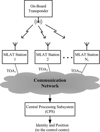
Multilateration (MLAT) systems are a powerful means for the surveillance function of air traffic control. These systems are intended to display to air traffic controllers the position and identification of aircraft (taxiing, taking off/landing, in the approach or en-route phases of flight) or of vehicles equipped with a Secondary Surveillance Radar (SSR) transponder [1]. To perform these functions, a number of ground stations (at least three for two-dimensional (2D) or four for three-dimensional (3D)), with capabilities to measure some characteristics of the mode-S signals, emitted by the transponders, such as Time of Arrival (TOA) and the enhanced or future systems; Round Trip Delay (RTD) and the Angle of Arrival (AOA) are placed in some strategic locations around the airport or around the area to be covered and connected with a Central Processing Subsystem (CPS), as sketched in Fig. 1.

Fig. 1. Generic MLAT system.
The accuracy of the position estimation in MLAT systems basically depends on the position of the stations [Reference Galati, Leonardi and Tosti2–Reference Torrieri5]. To design and deploy these systems, multiple factors such as the Line of Sight (LoS) of each station, the probability of detection, the accuracy, the redundancy, etc., must be considered. The main design goal is to deploy the minimum number of stations, in order to obtain the requested system coverage, meeting all the regulatory standards (e.g. those described in [1]), and the constraints imposed by each particular site, with a minimum cost. In general, choosing the number of stations and their locations to meet all the requirements is not an obvious task and the system designer has to make several attempts, by trial and error, before obtaining a satisfactory spatial distribution of the stations. As a matter of fact, the accuracy of the position of an aircraft (or vehicle) as reconstructed by an MLAT system depends on the measurements accuracy (in many cases, such measurements are TOAs) in each station and on the geometry, related to a factor called Dilution of Precision (DOP). This factor depends on the target position and on the positions of the MLAT stations contributing to the target localization. The related unknowns are the target's coordinates and the emission time for the transponder (the latter is eliminated by subtracting one TOA, i.e. by the Time Difference of Arrival (TDOA) technique). Therefore, for a 3D localization, there must be at least four visible stations and, in practice, to get acceptable accuracy levels and for redundancy reasons, the number of visible stations should be more than four.
The first application of the meta-heuristic optimization techniques to design MLAT systems was presented in [Reference Mantilla-G, Ruiz, Balbastre-T and Reyes6]. That work proposes the use of Genetic Algorithms (GAs) to obtain an optimal distribution (system geometry) of a fixed number of MLAT ground stations, but only taking into account the LoS and the DOP. However, there are other relevant parameters that should be taken into account in order to obtain a more realistic design. Another important aspect is that the DOP only reflects the errors due to the spatial distribution of the stations, regardless of other important sources of errors (e.g. errors due to propagation effects, which are site-dependent, instrumental errors due to time stamp, etc.).
This paper presents the evolution of the previous work [Reference Mantilla-G, Ruiz, Balbastre-T and Reyes6] with the introduction of more relevant parameters and a more rigorous and general methodology to evaluate the system accuracy (the Cramér–Rao Lower Bound (CRLB) analysis described in [Reference Galati, Leonardi and Tosti2]). The possible system improvement with other kinds of measurements, such as RTD [Reference Galati, Leonardi and Tosti2, Reference Perl and Gerry7] or AOA [Reference Galati, Leonardi and Tosti2, Reference Reck, Berold and Schmidt8], is also proposed and fully described. Moreover, the procedure developed herein is able to evaluate, validate, and improve previous system designs. On the other hand, a set of design strategies, to be used along with the procedure described here, is proposed and fully described.
The description of the general procedure is shown in Section II, then, in Section III, the set of design strategies with the simulation and results is shown. Finally, in Section IV, some conclusions and guidelines about the use of the general procedure are presented.
II. DESCRIPTION OF THE OVERALL DESIGN PROCEDURE
The procedure developed in this work is aimed at the designing of a standard MLAT system (e.g. with only TDOA measurements) or of its improved version (e.g. with the combination of TDOA/RTD or TDOA/AOA). In this work, the system design is obtained by calculating the minimum number of stations and their locations (site coordinates) that maximize the LoS coverage and the system accuracy. These calculations are performed under some regulatory constraints [1] or by those that are intrinsic to the airport layout, e.g. there are forbidden areas (clearances) or the available sites are restricted to some specific areas. In all cases, these constraints can be modified to satisfy some peculiarities of the design.
The procedure proposed here is also useful to analyze if any previous design is the optimum solution for a given resources or whether it could be improved by some feasible, but not obvious, position changes of the stations.
In this work, due to real constraints such as power supply, sites availability, etc., we have limited that search space only to a set of P sites in the airport area. The latter allows obtaining more realistic designs because only the actually available sites are used. In this case, the complexity of the problem, for a number of N s stations (with N s < P) can be evaluated by:
Equation (1) provides the number of possible combinations given the size of the discrete search space P and the number of stations to be deployed N s. On the other hand, when the aim is to obtain the possible minimum number of stations from a range R S = [N s1, N s2] and their positions, the complexity of the problem increases and can be evaluated by:

The general idea used here is based on the integration of different information and several numerical tools, in order to obtain a spatial distribution of the MLAT stations (number and site positions), which satisfies some requirements and restrictions. This idea is described in Fig. 2. This procedure needs information about the airport layout and the Digital Terrain Model (DTM); requirements such as system accuracy, system probability of detection (SPoD), system redundancy, and number of stations to be emplaced; design constraints or requirements such as the information about forbidden areas, the minimum spatial separation of the stations, and some regulatory constraints (e.g. those in ED-117 [1]). All this information is introduced in an iterative procedure, based on GAs that, in general sense, seeks to find the minimum number of MLAT stations and its optimum spatial distribution. This iterative procedure makes use of some numerical tools such as the CRLB analysis [Reference Galati, Leonardi and Tosti2], the model of MLAT errors, LoS calculation, and SPoD calculations.

Fig. 2. General frame for the procedure.
Moreover, in Fig. 2, there is another input called MLAT system. This input is needed for the analysis of possible system expansions or to validate if a previous system design is the most suitable option to satisfy the set of requirements and restrictions. This input has a corresponding output called System Expansion. This output contains all the information about the system expansion (new kind of measurements, new stations sites, etc.) or even a new system that satisfies all the requirements and limitations more effectively than the one at the input.
The procedure used in this work (based on that one proposed in [Reference Mantilla-G, Ruiz, Balbastre-T and Reyes6]) is shown in Fig. 3. This procedure is comprised of three steps, namely, Initialization (A), System Design Evaluation (B), and GA (C). In the following, these aspects are described.

Fig. 3. General design procedure.
A) Initialization
In this step, all the problem characteristics are defined. In the scenario definition, the P-set of possible sites to locate the stations is selected and some areas of interest (areas to calculate the system parameters –basically LoS and theoretical accuracy) are defined. Then, the initial station sites (normally by a random selection) and all the variables are initialized. The variables can be classified either as requirements or as restrictions. The requirements are the number of stations (or a range of minimum and maximum number), the horizontal accuracy and the SPoD [1]. All these are input data to the problem. On the other hand, the restrictions are the LoS redundancy, which is the minimum number of stations that must cover a point, in the coverage area, in order to satisfy the requirement of SPoD and the minimum spatial separation Δi,j between the ith and jth station. In this work, the restriction of LoS redundancy is calculated based on the manufacturer data about the PoD of each station. The SPoD, for a given point j, can be calculated as follows:

where PoD is the probability of detection of a single station (that should be provided by the manufacturer) and N sj is the number of stations that cover the jth point. In (3), it is assumed that at least four stations are needed to calculate the position. However, this condition can be easily changed. By (3), the minimum number of stations that make SPoDN sj equal or greater than the corresponding requirement for the SPoD can be estimated. This minimum value is taken as the LoS redundancy restriction. Moreover, this value also depends on the performance of the location algorithm used and in any case it can be modified (normally increased); in the rest of this work, we assume that the LoS redundancy calculated by the evaluation of (3) also satisfies the location algorithms performance.
B) System design evaluation
In the second step, the quality of the partial design is evaluated (i.e. the partial spatial distribution of the MLAT stations). For this, the LoS and the system accuracy are calculated (only in the areas of interest) and these values are introduced into a fitness function that assigns a suitable score and thus quantifies the quality of the partial system design, regarding the requirements and restrictions as defined in the first step.
The LoS calculation is performed only at the points within the areas of interest and the system accuracy is obtained by the CRLB analysis [Reference Galati, Leonardi and Tosti2] only at the points that satisfy the requirement of LoS redundancy. The CRLB analysis is a well-known technique in statistics, which sets a lower bound on the variance of an unbiased estimator. A full description of this technique can be found in [Reference Kay9] and the corresponding application to estimate the accuracy for MLAT systems is well described in [Reference Galati, Leonardi and Tosti2]. In this work, the CRLB formulation takes into account also the propagation effects, the instrumental errors, the synchronization errors, and the analog-to-digital converter rate and resolution [Reference Galati, Leonardi and Tosti2]. Moreover, the CRLB for each point is calculated with all the stations within the LoS for that point.
The quality of system design is evaluated and quantified by a fitness function (cost function) that takes into account the set of design requirements and restrictions, i.e. the technical and economic aspects. The technical aspects are related to satisfying the requirements and restrictions, and the economic aspects are related to the number of stations required to be used. This last aspect is useful to those simulations that seek to optimize the number of stations. The fitness function is specific to each problem but, in a general sense, the function proposed in this work takes the following form:

where cond is the total number of requirements and restrictions, c i is the cost of satisfying the ith requirement or restriction, and w i is a weight factor that controls the relevance of c i on the design. The corresponding values of w i and the functions to obtain c i, for each application are described in the next section.
C) GA
Finally, in the third step, a GA is used to iterate and modify the partial solution that will be evaluated by the iterative procedure described in Fig. 3. The GA used in this work is basically the same used in [Reference Mantilla-G, Ruiz, Balbastre-T and Reyes6].
The GA is a method for solving both constrained and unconstrained optimization problems that are based on natural selection, the process that drives biological evolution. The GA repeatedly modifies a population of individual solutions. At each step, the GA randomly selects individuals among the current population to be parents and uses them to produce the children for next generation. After successive generations, the population “evolves” toward an optimal solution [Reference Goldberg10]. This algorithm uses three main types of rules at each step to create the next generation from the current population: selection, crossover, and mutation rules. Selection rule selects the individuals, called parents, which contribute to the population at the next generation, crossover rule combines two parents to form children for the next generation, and mutation rule applies random changes to individual parents to form children.
The difference with respect to that algorithm applied in [Reference Mantilla-G, Ruiz, Balbastre-T and Reyes6] is that, due to the discretization of the search space to P possible options, here, an individual consists of an N s-array of integer numbers, where the value of the ith array position represents the index of the selected site for the ith station. Moreover, it is worth saying that the information contained in a specific individual position can change and depends on the parameters to be optimized in the design. This particularity and the corresponding notation are commented in the next section.
Finally, it is worth saying that the GA has been chosen for this work because this is one of the most well-established meta-heuristic optimization methods, which can be found in the literature. The full description and analysis of this method are beyond the scope of this work, but, the interested reader can find a full description of this algorithm in [Reference Goldberg10, Reference Sivanandam and Deepa11]. Furthermore, due to the modularity of the procedure proposed herein (see Fig. 3), its extension to any other optimization method, such as Particle Swarm Optimization (PSO) [Reference Clerc12] or Ant Colony Optimization (ACO) [13], is straightforward.
III. SIMULATION AND RESULTS
To validate the procedure proposed in this work, three different simulations (one for every proposed strategy) have been carried out over the layout of Barcelona (Spain) Airport. The common objective for all the simulations is to obtain an MLAT system that covers the three runways, the taxiways, and the apron centrelines, given a set of requirements and restrictions. The first simulation consists of the design of an MLAT system with a fixed number of TDOA stations. The second one consists of the design of an MLAT system with a variable number of TDOA stations. In this simulation, the objective is to find a design that satisfies all the requirements and restrictions by using the possible minimum number of TDOA stations. The last simulation consists of the design of an MLAT system with a fixed number of TDOA and AOA stations. Figure 4 shows the Barcelona airport layout and the P-set of available sites for the simulations. For these simulations, P = 41.

Fig. 4. Barcelona airport layout with the P-set of available sites (circles).
For all the simulations, the antenna station height (mast length) has been assumed to be equal to 2 m and the calculations for LoS and CRLB are performed for a spatial grid of 5 m × 5 m. This spatial grid is also in agreement with the DTM used to calculate the LoS. The GA parameters (Table 1) for all the simulations are described subsequently.
Table 1. Parameters for GA.

A) MLAT system with a fixed number of TDOA stations
The first scenario shows the first and the standard strategy proposed herein to be used along with the procedure of Fig. 3. It consists of the design of a standard MLAT system for a given set of requirements and restrictions. The requirements for this particular simulation are based on those described in [1], which are basically: horizontal accuracy must be within 3.75 m (σ) and the SPoD must be better than 99.9%. The number of stations to use in this design is 12 and they measure the TDOA. The restriction of LoS redundancy, using a station probability of detection of PoD = 97%, provided by a quick evaluation of (3) is 7 and the minimum spatial separation is set to Δmin = 400 m.
For this scenario, an individual is an array of 12 × 1 size, where the ith position represents the index of the possible position for the ith station and it can be written as x = [p l, …, p m]T, where p l and p m are elements of the search space, i.e. the P-set of available sites shown in Fig. 4. The fitness function for this scenario takes the following form:
where f TC is a function that quantifies the requirement of total coverage for a partial solution xt at time t, i.e. the percentage of points that are covered for more than LoS redundancy stations within a horizontal accuracy better than the corresponding value defined in the requirements and, f RoS is a function that quantifies the restriction of minimum spatial separation between two stations for a partial solution xt at time t. These two functions can be calculated as follows:
and
Finally, the value of the weight factors depends on the importance given to each requirement or restriction on the design; they can be chosen by the designer, taking into account that the weight factor associated with the total coverage, e.g. w 1 for this case, must be much greater than the other ones; normally greater than 0.8. Here, we have used w 1 = 0.95 and w 2 = 0.05, and in the remaining part of the paper the same reasoning is used to define these weight factors. The only condition that must be satisfied is that the sum of these must be equal to 1. The function in (7) penalizes those solutions with stations close to each other at a distance smaller than Δmin. However, there exists the possibility of obtaining solutions with two (or more than two) stations in the same site. These particular situations are penalized directly in (5) instead than in (7). In this way, the final expression for the fitness function takes the following form:
where F R1(xt) = w 1f TC(xt) − w 2f RoS(xt).
Figure 5 shows the horizontal accuracy for this scenario and how the interested areas of interest are covered with the assumed requirements. From the theory [Reference Galati, Leonardi and Tosti2, Reference Levanon4, Reference Torrieri5] it is well known that a convenient system geometry, to obtain high-accuracy levels, is to set the stations in a polygon enclosing the area of interest. In Fig. 5, it can be observed that the proposed procedure provides a solution that agrees with this theoretical aspect. Finally, Fig. 6 shows the procedure convergence. In this scenario, the number of possible combinations, provided by (1), is 7.8987 × 10⁹ and a relative good solution is obtained within 50 iterations, which means only 500 problem evaluations. At this number of iterations, it can be considered that the procedure has been converged. However, it is advisable to expend more iterations (up to 200) because the random component of the GA allows the procedure to explore new values in the search space. It is also important to emphasize that, sometimes, this random component can move the mean fitness value (line with circles in Fig. 6) to a worst value, but because this procedure always save the best solution (best fitness value), it does not represent a problem in the algorithm convergence. In any case the total number of problem evaluations is significantly much smaller than that value provided by (1). The latter justifies the use of this procedure instead of the full evaluation of the problem.

Fig. 5. Horizontal accuracy for the design with a fixed number of TDOA stations.

Fig. 6. GA convergence for the design with a fixed number of TDOA stations.
B) MLAT system with a variable number of TDOA stations
The second scenario consists of the design of an MLAT system with a variable number of TDOA stations. In this kind of scenario, the objective is not only to define the stations sites but also to calculate a relative minimum number of stations that satisfies all the assumed requirements and restrictions. In other words, to estimate the minimum number of stations that provides the maximum coverage with the maximum accuracy levels. All the requirements and restrictions for this problem are those described for the first problem. Moreover, for this problem, it is necessary to stipulate a range for the number of stations. For this work, a range of R N s = [7,15] has been used.
For this scenario, an individual is an array of variable length, where the first position sets the array length. It can be written as x = [N st, p l,…, p m]T, where N st is the number of stations calculated at time t. The fitness function for this scenario takes the following form:
where F R 2(xt) = w 1f TC(xt) − w 2f RoS(xt) − w 3f RoNS(xt) and f RoNS is a function that quantifies the cost of satisfying the requirement of number of stations. This function is expressed as follows:
Finally, the weight factor values used for this problem are w 1 = 0.85, w 2 = 0.05, and w 3 = 0.1.
Figure 7 shows the results for the horizontal accuracy. Also, in this scenario, all the areas of interest are covered satisfying all requirements and restrictions. The important aspect in this scenario is that the minimum number of stations calculated is 11, it is one station less than in the first scenario. This kind of simulation is useful to know an approximate minimum number of stations that meets the requirements and restrictions. However, due to the random component of the GA, it is advisable to run the procedure, for this scenario, once or twice more, just to validate the calculated minimum number. Finally, Fig. 8 shows the procedure convergence for this scenario, where a good solution is found after 150 iterations. It can be understood because the complexity of this problem (number of possible combinations, see (2)) is much greater (1.2894 × 10¹¹) than that of the first scenario.

Fig. 7. Horizontal accuracy for the design with a variable number of TDOA stations.

Fig. 8. GA convergence for the design with a variable number of TDOA stations.
C) MLAT system with a fixed number of TDOA/AOA stations
This scenario consists of the design of an enhanced MLAT system with a fixed number of TDOA/AOA stations. The AOA stations, for this case, measure the elevation (vertical) AOA. Normally, the elevation AOA measurement capabilities are added to improve the horizontal accuracy in surface movement applications [Reference Galati, Leonardi and Tosti2]. For this scenario, the requirements and restrictions are those described for the first problem and the AOA measurements capabilities are added only to the station number 1 (the AOA measurements error is assumed to be 10−3 rad).
For this scenario, an individual is represented as in the first scenario, i.e. as an array of 12 × 1 size x = [p l, …, p m]T. The difference lies in that, for this scenario, the pertaining LoS coverage of the station number 1 is relatively more important than those of the remaining stations. This particular aspect is introduced in the fitness function as follows:
where F R 3(xt) = w 1 f TC(xt) + w 2 f LoS(xt(1)) − w 3 f RoS(xt) and f LoS is a function that quantifies the relative LoS coverage of the station number 1 and it can be calculated as follows:
Finally, the weight factor values used for this problem are w 1 = 0.9, w 2 = 0.05, and w 3 = 0.05.
The usefulness of this strategy is justified because it is not enough to add the AOA measurement to that station with the highest percentage of LoS coverage (e.g. that in the first strategy A). Moreover, it is also important to optimize the location of the TDOA/AOA station because this significantly influences the overall system accuracy [Reference Galati, Leonardi and Tosti2].
Figure 9 shows the horizontal accuracy for this scenario. The complexity of this problem is basically of the same order than that of the first one but, here the CRLB calculation has been carried out by taking into account the accuracy improvement provided by the TDOA/AOA station [Reference Galati, Leonardi and Tosti2]. The final site for this station is shown in Fig. 9 as a diamond. Also, for this kind of scenario, it is advisable to run the procedure once or twice more. Similar to the first problem, here a good solution is found after 50 iterations (see Fig. 10) and also at this number of iterations it can be considered that the procedure has been converged. Moreover, also for this case, due to the additional iterations, it can be observed that the mean fitness value (line with circles in Fig. 10) is moved to slightly higher values for iterations between 60 and 80, but, after that, it decreases and approximately maintains a constant value after 100 iterations.

Fig. 9. Horizontal accuracy for the design with a fixed number of TDOA/AOA stations.

Fig. 10. GA convergence for the design with a fixed number of TDOA/AOA stations.
IV. CONCLUSION
In this work, an efficient procedure to define the layout of standard and enhanced mode-S MLAT systems has been presented. This procedure is based on the use of GAs along with the integration of different information and several numerical tools such as the general CRLB analysis. Moreover, a set of practical and useful strategies to apply the procedure are also proposed and fully described. They are useful not only to design new standard and enhanced MLAT systems but also to validate whether a previous system design could be the optimum solution with regard to a set of available resources and to analyze possible system expansions.
The procedure and strategies shown in this work are very useful because it avoids the full evaluation of all the possibilities. Instead of this, it has been found that only the evaluation of the 6 × 10⁻⁶% of all the possible options is enough to obtain satisfactory results, i.e. a system design that satisfies all the requirements and restrictions.
Three kinds of designs have been presented. The first one is able to design new MLAT systems with a fixed number of TDOA stations but also to validate whether a final design (clearly before the implementation) can be improved by feasible, but not obvious, site changes. The second one provides a strategy to obtain a minimum number of stations that satisfy all the stipulated requirements and restrictions. The third one is proposed to design enhanced MLAT systems, i.e. by using other type of measurements such as AOA or RTD. For the third design, an example with an MLAT system using TDOA/AOA stations has been presented, but the use with other measurements combinations is straightforward. Finally, it is worth saying that also these design strategies can be used together to obtain more reliable results, e.g. firstly the second design can be used to obtain a possible minimum number of stations that meets all the requirements and restrictions and then, by means of the first design (or the third one in the case of enhanced MLAT systems), obtain the optimum sites or just to validate the set obtained with the second one.
The use of new requirements or restrictions is also possible only by simply modifying the corresponding cost function and their weight factors.
ACKNOWLEDGEMENT
Mr Ivan A. Mantilla-Gaviria has been supported by an FPU scholarship (AP2008-03300) from the Spanish Ministry of Education.
 Ivan A. Mantilla-Gaviria was born in Bucaramanga, Colombia in 1985. He received the Degree in Telecommunications Engineer (Cum Laude) from Saint Thomas University, Bucaramanga, Colombia, in 2006 and the Master of Science degree in Technologies, System, and Communications Network from Polytechnic University of Valencia (UPV), Valencia, Spain, in 2007. In December 2006, he joined the ITACA (Institute for the Application of Advanced Information and Communication Technologies) Research Institute as Ph.D. student in the Electromagnetism Applied Group, where he has collaborated in several R&D projects with companies and public administrations in radar applications, and design and quality control of software. In 2009, he joined the Communication Department at UPV as a researcher with FPU scholarship from the Spanish Ministry of Education, where currently he also teaches navigation systems laboratory. His main research interests include radar topics and optimization methods.
 Mauro Leonardi was born in 1974, in Rome, Laurea cum laude in Electronic Engineering (May 2000) at Tor Vergata University in Rome. He received a Ph.D. in October 2003, focusing his work on Target Tracking, Air Traffic Control, and Navigation. From January 2004, he is Assistant Professor at Tor Vergata University in Rome where he teaches “Detection and Navigation Systems” and “Radar Systems”, his main research activities are focused on: Air Traffic Control and Advanced Surface Movement Guidance and Control System (A-SMGCS); Satellite Navigation, Integrity, and Signal Analysis. He is the author/co-author of over 25 papers, two patents, and many technical reports.
 Gaspare Galati from 1970 till 1986 was with the company Selenia, where he was involved in radar systems analysis and design. From March 1986, he is associate professor (full professor from November 1994) of Radar Theory and Techniques at the Tor Vergata University of Rome, where he also teaches Probability, Statistics, and Random Processes. He is senior member of the IEEE, member of the IEE, and of the Associazione Elettrotecnica ed Elettronica Italiana, AEI. Within the AEI he is the chairman of the Remote Sensing, Navigation, and Surveillance Group.
 Juan V. Balbastre-Tejedor was born in Mislata, Spain, in August 1969. He received the Engineering and Ph.D. degrees from the Polytechnic University of Valencia, Valencia, Spain, in 1993 and 1996, respectively. Since 1993, he has been a member of the research and teaching staff in the Department of Communications at the Polytechnic University of Valencia. In 2001, he joined the research staff of the ITACA Research Institute, Polytechnic University of Valencia. From 1998 to 2006, he was the Academic Vice-Dean at E.T.S.I. Telecomunicación of Valencia, Valencia. His current research interests include electromagnetic theory and computational electromagnetic applied to industrial microwave systems, electromagnetic compatibility, and radar. Currently, he is the Director of the E.T.S.I. Telecomunicación of Valencia, Valencia.
 Elías de los Reyes Davó was born in Albatera, Spain, in 1950. He received the Engineering degree from the Polytechnic University of Madrid (UPM), Madrid, Spain, in 1974 and the Ph.D. degree from Polytechnic University of Catalunya (UPC), Barcelona, Spain, in 1978. From 1974 to 1988, he was with the E.T.S.I.T. of the UPC, Barcelona, Spain, as a full professor. Since 1988, he has been a full professor in the Communication Department at the Polytechnic University of Valencia (UPV), Valencia, Spain, where he has taught electromagnetic fields and Radar. Currently he is the Director of the Applied Electromagnetism Group at the ITACA Research Institute in UPV. He has published several books on electromagnetism and numerous (more than 100) national and international papers, having received the favorable assessment of his research by the ANECA (National Quality Assessment Agency) in several 6-year assessment exercise periods. His current research interests include electromagnetic theory, microwave heating, and radar applications.