


I. INTRODUCTION
In recent years, the interest in using millimeter-wave radar sensors for civil applications has increased significantly. Because of their day and night operability and robustness in harsh environments, radar systems are ideally suited for numerous applications [Reference Menzel1–Reference Brooker, Widzyk-Capehart, Scheding, Hennessy and Lobsey3]. Besides the classical targets' range and velocity measurements, the deployment of multiple channels in a radar system adds the advantage of measuring the angular position of targets. Such a radar system uses an array of antennas in order to synthesize virtual beams. It simultaneously scans the whole space by means of digital signal processing without the need for mechanical beamsteering [Reference Savelyev4–Reference Mayer, Buntz, Leier and Menzel6]. Compared to phased array systems this so-called digital beamforming technique offers a more flexible and cost-efficient electronic scanning technique [Reference Steyskal7, Reference Weiss8].
In this paper, the proposed three-dimensional (3D) measurement principle deploys a frequency-modulated continuous wave (FMCW)-based multi-channel radar system in combination with digital beamforming. Besides digital beamforming on receive, the realized 24GHz digital beamforming radar provides several additional transmitter channels for digital beamforming on transmit [Reference Harter, Kornbichler and Zwick9]. For the acquisition of the angular information in azimuth and elevation, the transmit and receive antenna arrays are arranged orthogonal to each other [Reference Mills and Little10, Reference Kraus11]. The combination of the so-called T-shaped antenna array arrangement with the multiple-input multiple-output (MIMO) technique is an advantageous method for two-dimensional beamforming [Reference Harter, Ziroff and Zwick12, Reference Asano, Ohshima, Harada, Ogawa and Nishikawa13].
The paper is organized as follows: In the first section, the proposed 3D measurement concept by digital beamforming is described in detail, along with the signal processing approach based on the FMCW principle and the conventional delay-and-sum beamformer. The realization of the 3D imaging radar hardware at 24GHz and aspects concerning the array calibration are presented in Section III. In the final section, the performance of the 3D imaging radar system is successfully demonstrated by measurements of several scenarios.
II. 3D IMAGING by DIGITAL BEAMFORMING
A) Concept and realization
3D imaging of a scenario requires range and angular information in azimuth and elevation. By means of the FMCW measurement principle the target's range is provided, whereas the angular information is acquired by digital beamforming. The proposed 3D measurement concept uses two antenna arrays with M transmitter and N receiver antennas. With an orthogonal arrangement of the two antenna arrays in the form of a T, the azimuth and elevation angles can be determined by digital beamforming in two dimensions.
As shown in Fig. 1, the measurement of the azimuth angle ψ is performed with N receiving antennas, located uniformly in x-direction with a spacing of d x. The receiver channels allow simultaneous reception. The elevation angle θ is determined by digital beamforming on transmit, with the antenna array aligned along the z-direction with an antenna spacing of d z. It is necessary to distinguish the signals coming from different transmitter antennas on receive in order to exploit the signal information from each transmitter and receiver combination. This can be achieved by operating the transmitter channels in time-division multiplexing (TDM). In this mode, only one transmitter is active during one FMCW sweep, while the other transmitter channels are switched off. After each FMCW sweep f m, the transmitters are switched (Fig. 2a). The switching time segment t m for each transmitter m consists of the switching time from one transmitter to the next and the FMCW sweep duration T S. After one complete transmit cycle, in which the signal is switched successively from transmitter 1 to M, the elevation angle can be determined. In contrast to the transmitter switching, the range and the azimuth angle can be directly processed after each FMCW sweep due to the simultaneous operation of the receiver channels (Fig. 2b).

Fig. 1. Orthogonal arrangement of transmit and receive antennas as a T-shaped array for 3D imaging.
Fig. 2. Signal processing flow for 3D imaging with (a) sequential switching of transmitters and (b) simultaneous acquisition on receive.
The applied T-shaped antenna array arrangement is an advantageous technique for 3D imaging with a minimum number of antennas. Further, the hardware effort is highly reduced by using digital beamforming on transmit in one spatial direction instead of additional receiver channels.
B) Signal processing
Assuming far-field conditions for the FMCW-based radar system, a simplified signal model can be given according to Stove [Reference Stove14]. After a discretization of the continuous time t by taking p discrete time samples during the sweep duration T S, the down-converted and low-pass-filtered intermediate frequency for a single static target can be written as
The variable p = 0, 1, . . . , P − 1 is the discrete time index, A the target's radar cross-section-dependent amplitude of the received signal, f 0 the initial sweep frequency, B the sweep bandwidth, and r k the distance between the antenna array reference point and the target. Further, the propagation velocity of the electromagnetic wave is given by c 0 and the target-dependent signal phase by φ.
According to Fig. 1, the signal model can be extended to the MIMO case as the traveling distance r tr of the electromagnetic wave is composed of the distance between transmitter m to the target k and the distance from the target back to receiver n:
where
is the distance between the transmit antenna element m, which is located in the z-direction and the target located at (x k, y k, z k). The distance from the target to the receiver antenna elements, which are arranged in the x-direction, is
![\eqalign {r_r \left[n \right]&=\sqrt {\left({\mathop {\left({ld_x - x_k } \right)}\nolimits^2+y_k^2+z_k^2 } \right)}\cr & \quad \quad \hbox{with}\quad l=- \displaystyle{{N - 1} \over 2}\comma \; \ldots\comma \; +\displaystyle{{N - 1} \over 2}.}\eqno \lpar 4\rpar](https://static.cambridge.org/binary/version/id/urn:cambridge.org:id:binary:20151130141431726-0178:S1759078712000414_eqn4.gif?pub-status=live)
Expanding the square roots in a binominal series and preserving only the constant and linear terms for far-field approximation [Reference Steinberg and Subbaram16], the distances can be given by
and
![\eqalign{r_r &\left[n \right]=r_k+ld_x \sin \psi \quad \quad \cr &\hbox{with}\quad l=- \displaystyle{{N - 1} \over 2}\comma \; \ldots\comma \; +\displaystyle{{N - 1} \over 2}\comma \;} \eqno \lpar 6\rpar](https://static.cambridge.org/binary/version/id/urn:cambridge.org:id:binary:20151130141431726-0178:S1759078712000414_eqn6.gif?pub-status=live)
where r k is the target distance to the reference point. Thus, the signal model in (1) can be extended as follows:
where
defines the time-varying frequency sweep of the transmit signal. In the case of multiple targets, the signal model in (7) contains the sum of the reflected signals.
The so-called delay-and-sum beamformer is a way to recover the angular information in azimuth and elevation direction of the reflected signal and is applied in the following. Range and azimuth processing can be directly started after one FMCW sweep as the reflected signal of transmitter m is measured by all receiver channels simultaneously. After one complete transmit cycle, the full 3D signal array s MIMO [p, m, n] is acquired. With these data, the angular information in elevation can be determined by digital beamforming on transmit.
Figure 2 shows the signal processing steps for 3D imaging. In the first step, range compression is applied in which the information of each transmitter – receiver combination is compressed into P-range cells by using the fast Fourier transform (FFT):
![\eqalign {S_{mn} \left[{q\comma \; m\comma \; n} \right]&=\sum\limits_{p=0}^{P - 1} \, s_{MIMO} \left[{p\comma \; m\comma \; n} \right]e^{ - jpq\;{\textstyle{{2\pi } \over P}}}\comma \; \cr \quad q&=0\comma \; \ldots\comma \; P - 1.}\eqno \lpar 9\rpar](https://static.cambridge.org/binary/version/id/urn:cambridge.org:id:binary:20151130141431726-0178:S1759078712000414_eqn9.gif?pub-status=live)
The applied FFT delivers a total of M × N complex data points in each of the range cells. In the second step, the azimuth angle ψ is determined by digital beamforming over N parallel receiver channels:
![S_{mn} \left[{q\comma \; \psi\comma \; m} \right]=\sum\limits_{l=- {\textstyle{{N - 1} \over 2}}}^{{\textstyle{{N - 1} \over 2}}} \, S_{mn} \left[{q\comma \; m\comma \; n} \right]e^{ - j\,{\textstyle{{2\pi } \over \lambda }}\;{\textstyle{{ld_x sin\psi } \over N}}}.\eqno \lpar 10\rpar](https://static.cambridge.org/binary/version/id/urn:cambridge.org:id:binary:20151130141431726-0178:S1759078712000414_eqn10.gif?pub-status=live)
The unambiguous measurement range in azimuth can be defined according to [Reference Schuler, Younis, Lenz and Wiesbeck5]
With digital beamforming on transmit, the angular information in elevation can be obtained by applying the FFT as follows:
![S_{mn} \left[{q\comma \; \psi\comma \; \theta } \right]=\sum\limits_{m=1}^M \, S_{mn} \left[{q\comma \; \psi\comma \; m} \right]e^{ - j\;{\textstyle{{2\pi } \over \lambda }}\;{\textstyle{{md_z sin\theta } \over M}}}.\eqno \lpar 12\rpar](https://static.cambridge.org/binary/version/id/urn:cambridge.org:id:binary:20151130141431726-0178:S1759078712000414_eqn12.gif?pub-status=live)
Equally to (11), the unambiguous measurement range in elevation can be determined. Zero padding can be used for interpolation of the spectra. For better sidelobe suppression, window functions are applied before range and angular processing, whereas broadening of the main beam has to be taken into account [Reference Harris15].
III. SYSTEM REALIZATION
A) Hardware prototype
In order to demonstrate the above described 3D imaging principle, a 24GHz radar system for 2D beamforming was built [Reference Harter, Kornbichler and Zwick9]. With this system, the 3D imaging capabilities can be tested and evaluated for different measurement applications in a real-world environment. Both the number of transmitter and receiver channels is chosen to eight, as this is found to be a good compromise between hardware effort and achievable angular resolution. For a maximum of flexibility, the hardware architecture is divided into four main modules as shown in the block diagram in Fig. 3. As it can be seen from the photograph in Fig. 4, the modules are realized on separate printed circuit boards (PCBs) which are arranged as a modular platform stack. The advantage of this compact modular assembly is that it allows a quick reconfiguration and further optimization of the radar system.

Fig. 3. Block diagram of the realized digital beamforming hardware.

Fig. 4. Radar hardware realized as a modular stack.
The transmit signals, as well as the local oscillator signal for the receiver module are generated from a commercially available voltage-controlled oscillator (VCO) controlled by a phase-locked loop (PLL). The reference for the PLL is the output of a programmable direct digital synthesis (DDS) signal generator which is clocked by a stable reference crystal oscillator (RCO). In combination, this setup forms a frequency synthesizer providing FMCW signals with freely programmable sweep frequencies and slopes.
The transmitter module consists of eight independently switchable transmitters. Each transmitter is supplied with the signal generated by the VCO divided by a power divider network, consisting of seven Wilkinson dividers. The switching of each transmitter is realized by controlling the power supply of a three-stage low-noise amplifier (LNA) at the end of the Wilkinson divider network. In the ‘on’ state, all three amplifier stages are supplied with power, whereas in ‘off’ state, the power supply of the second and third stage is switched off. The first amplifier stage is active all the time for matching purposes, maintaining low return loss. For further explanation of the switchable amplifier design refer to [Reference Harter, Kornbichler and Zwick9]. With this realization, a switching time of less than 100 ns can be achieved which is negligible in comparison with the sweep duration. In the realized design, the LNA provides a total gain of 18 dB and an output power of typically 10 dBm in ‘on’ state. The return loss and isolation in ‘off’ state are measured to −14.5 dB and −32 dB at 24 GHz, respectively.
The receiver module allows the coherent reception and processing of the radar signal with eight parallel receiver channels. Each receiver channel includes an LNA for power amplification, a double-balanced mixer for down-conversion, and an active band-pass filter. The local oscillator signal for all eight mixers is provided from the synthesizer module which is distributed through a Wilkinson divider network. All eight down-converted beat frequencies are sampled and digitized by one integrated analog-to-digital converter (ADC). The ADC includes track-and-hold circuitry for simultaneous sampling of eight input channels and provides a sample rate of up to 250 kS/s per channel, with a resolution of 14 bits.
The system control and data read-out are performed by a Virtex-4 field programmable gate array (FPGA) board from Xilinx. The FPGA module is placed at the bottom of the hardware stack. The realized system architecture is divided into a function block for time-sensitive operations, implemented by the hardware description language VHDL and an embedded soft-core processor design as presented in [Reference Harter and Zwick17]. The switching of the transmitter channels and the protocol handling of the ADC are implemented as VHDL modules in order to meet the timing and clock requirements.
The acquired data from the ADC are buffered in a double-data-rate-synchronous dynamic random access memory (DDR-SDRAM), provided on the FPGA board. With its memory size and the parameters shown in Table 1, up to 6000 FMCW sweeps can be sampled consecutively, which corresponds to an acquisition period of about 15 s. This time span is sufficiently long for the acquisition of scenarios with moving targets.
Table 1. System and measurement parameters.
By using the on-board Ethernet physical transceiver device (PHY), a TCP/IP connection between the FPGA board and a PC is established, allowing data transfer rates of up to 100 Mbit/s.
The data are imported to Matlab, which is also used for configuring and controlling the radar system. In Matlab, the signal processing is performed based on the raw ADC data. However, the remaining free resources of the FPGA allow the implementation of algorithms in hardware so that real-time and stand-alone applications could also be realized with the presented system.
B) Patch antenna arrays
The results from the previous sections show how a MIMO radar in combination with orthogonally arranged antenna arrays can be used to localize targets in a 3D space. The proposed T-shaped antenna array configuration, shown in Fig. 1, implies that the transmitter and receiver antennas provide the same polarization. Furthermore, a similar field of view as well as a similar angular resolution in azimuth and elevation are intended.
Thus, each individual antenna element of the described arrays is designed as a 2 × 2 patch antenna that provides a half-power beamwidth of 42° in azimuth and 50° in elevation. From the photograph in Fig. 5, it can be seen that eight 2 × 2 patch antennas are arranged uniformly along the z-direction with a spacing of d z = 14.2 mm as a transmitter array. Likewise for the receiver antenna array, eight 2 × 2 patch antennas are located horizontally with an equal spacing of d x = 14.5 mm. In order to reduce direct coupling of the transmitted signals into the receiver channels, the antenna arrays are positioned with an offset of 3d x to each other.

Fig. 5. Complete system with patch antennas attached.
The radiation patterns of the realized antenna arrays are measured in an anechoic chamber and compared with the simulated arrays. For the measurements, all single elements have to be fed uniformly by one signal source. Therefore, a separate PCB with seven Wilkinson dividers for power division was built. Exemplarily, the measured and simulated radiation pattern of the transmitter array with eight 2 × 2 patch antennas is shown in Fig. 6.

Fig. 6. Simulated and measured radiation patterns of the transmitter array. Tapered transmit array patterns with a Dolph–Chebyshev window of 20 dB and 40 dB sidelob suppression.
Deviations in the sidelobe regions between the simulated and the measured radiation patterns can be explained by the hardware imperfections of the Wilkinson divider network, resulting in an unequal power distribution between the transmitters. From Fig. 6, the half-power beamwidth of the simulated and measured transmit array pattern can be determined to 5.5° and 5.8°, respectively. Digital beamforming has the advantage that a reduction of sidelobes can be achieved by window functions during signal processing. Therefore, the amplitude-tapered radiation patterns with a Dolph–Chebyshev window with a sidelobe suppression of 20 dB and 40 dB are shown in Fig. 6 as well [Reference Harris15]. Due to the applied window, a broadening of the main beam can be observed. Grating lobes occur in the region of −60° and +60°. They are the limiting factor of the unambiguous measurement range in such a beamforming system. The theoretical unambiguous measurement range in elevation, which is calculated according to equation (11) from −26.1° to +26.1°, is drawn in Fig. 6. In Fig. 7, the measured responses of a corner reflector placed at 0° and +26° are shown. It can be seen that the target at +26° causes an ambiguity.

Fig. 7. Measured responses of a corner reflector placed at 0° and +26° in elevation with an applied Dolph–Chebyshev window function of −13 dB sidelobe level.
A similar radiation pattern with a half-power beamwidth of 5.3° determined by simulation and 6° by measurement is retrieved for the receiver antenna array. In comparison with a full planar array with M × N antennas, a broader half-power beamwidth, higher sidelobe levels, and a lower gain have to be taken into account when using the T-shaped array configuration with only M × N antennas.
C) Calibration
The performance of a digital beamforming radar system can be deteriorated due to amplitude and phase imbalances as well as by mutual coupling between the channels. These errors have several effects on the beamforming result, as e.g. beam skew and broadening, and make a sensor calibration essential. Mutual coupling occurs mainly between the antennas. In the presented 3D imaging radar system, mutual coupling between the antennas was measured on a level lower than −35 dB. Compared to the amplitude and phase errors, mutual coupling has a minor impact on the performance and is neglected in the calibration procedure of the presented radar system. Much more effect shows a correction of the amplitude and phase errors of the channels which originates mainly from manufacturing tolerances. The applied phase correction procedure is presented in [Reference Harter, Chaudhury, Ziroff and Zwick18]. During this calibration procedure, a phase correction term for each transmitter and receiver channel is estimated by measurements of a strong corner reflector at different positions in front of the radar system.
IV. MEASUREMENT RESULTS
In order to demonstrate the functionality and applicability of the 3D imaging principle, several characteristic measurements with the realized digital beamforming radar hardware presented in Section III are performed. In Table 1, the system and measurement parameters are given. The calibration data obtained from the described calibration procedure in the previous section are applied throughout the presented measurements. In the following, the measurements are carried out with a corner reflector with a radar cross section of σ ≈ 2 mReference Tokoro2.
A) Accuracy
First, the achievable system accuracy of the radar system is investigated. For the measurement of the range accuracy, a corner reflector is placed at distances between 2 m and 9 m to the radar system. In Fig. 8, the measurement error is plotted over the measured ranges. From this measurement a maximum error of about 3 cm is obtained.

Fig. 8. Measurement error in range.
The measurements for the evaluation of the angular accuracies are performed in an anechoic chamber. Therefore, a corner reflector is placed in front of the radar system at a fixed position and the radar system is attached to a rotating tower. The measurements of the angular errors in azimuth and elevation are shown in Fig. 9, where the tower is rotated in steps of 5°. A small angular measurement error can be observed in the region of −5° to +5° for both directions, whereas the angular errors increase in the outer regions. This results from the limited calibration data. The applied phase correction terms are obtained from measurements of a corner reflector, which is placed at different ranges in front of the radar system with an angular orientation of 0°. A further improvement of the angular accuracy can be achieved by a direction-dependent calibration procedure.

Fig. 9. Angular measurement error.
B) Resolution
The angular resolution capability of the presented radar system with a T-shaped antenna array is verified by measurements of two closely spaced corner reflectors in the anechoic chamber (Fig. 10). The used corner reflectors with same radar cross sections are both placed in a distance of 4 m in front of the radar sensor. For the measurement of the angular resolution in elevation, the whole radar system is turned by 90°.

Fig. 10. Measurement setup with two corner reflectors for verification of the angular resolution.
The measurement results are shown by 2D plots in Figs 11 and 12, respectively. The achieved angular resolutions are very close to the measured half-power beamwidths given in Section III. A Dolph–Chebyshev window function with a −13 dB sidelobe level is applied to the measured data in elevation and azimuth direction. Despite the applied window function, not all sidelobes can be suppressed under −13 dB.
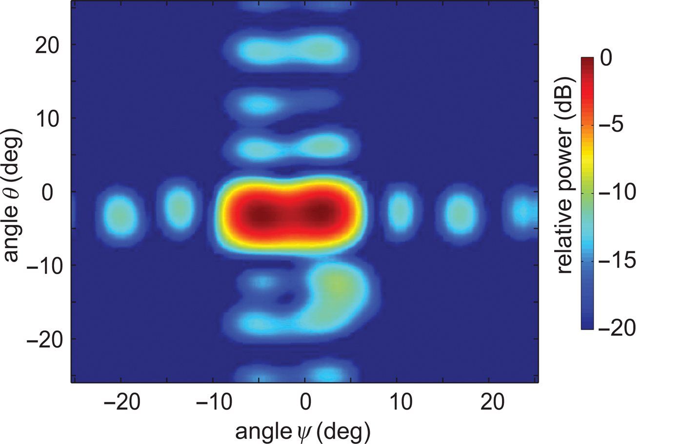
Fig. 11. Measured angular resolution in azimuth.

Fig. 12. Measured angular resolution in elevation.
The theoretical resolution in range can be calculated to δ r = 0.56 m by the given bandwidth in Table 1. A range resolution of 0.65 m is achieved with an applied Dolph–Chebyshev window of −40 dB sidelobe level by a measurement of two corner reflectors in the same angular direction.
C) 3D Measurement
Finally, a measurement for the demonstration of the 3D target detection capability of the radar system is shown. For this purpose, an outdoor measurement scenario with two corner reflectors placed at different distances and heights is chosen (Fig. 13). In Fig. 14, the 3D imaging result is shown by a volumetric slice representation with 2D color coded slices at the range positions of the corner reflectors. The two corner reflectors at the positions (r 1, ψ 1, θ 1) = (6 m, 12°, 4°) and (r 2, ψ 2, θ 2) = (9 m, −6°, −5°) can be clearly identified in Fig. 14 and verify the presented 3D imaging principle.

Fig. 13. Outdoor measurement setup with two corner reflectors at different distances and heights.

Fig. 14. 3D measurement result of the two corner reflectors in a volumetric slice representation.
V CONCLUSION
An innovative radar system for 3D object detection and imaging is presented in this paper. The proposed 3D imaging principle, based on 2D digital beamforming, is covered and aspects regarding the associated signal processing are outlined. Finally, the 3D imaging concept and the functionality of the realized 24GHz radar system are successfully demonstrated and proven by measurements. Due to the combination of the MIMO principle and the T-shaped antenna array, in which the transmitter and receiver antenna arrays are arranged orthogonal to each other, 2D beamforming is performed with a minimum number of antennas. Further, the hardware effort is highly reduced by introducing digital beamforming on transmit in one scan direction.
The presented 3D measurement concept in its realization opens new opportunities for a large number of applications.
 Marlene Harter received the Dipl.-Ing. (M.S.E.E.) degree in electrical engineering from the Universität Karlsruhe (TH), Germany in 2008. She is currently working towards her Dr.-Ing. (Ph.D.) degree at the Institut für Hochfrequenztechnik und Elektronik (IHE) at the Karlsruhe Institute of Technology in cooperation with Siemens AG in Munich, Germany. Her main research interests include radar signal processing as well as radar system design and concepts for industrial and security applications. Ms. Harter received the Excellent Paper Award at the IEEE CIE International Conference on Radar in 2011.
 Tom Schipper Tom Schipper received his Dipl.-Ing. (FH) degree in communications and electronic engineering from the University of Applied Sciences Mannheim, Germany in 2008 and one year later received the M.Sc. degree from the same institution. He is currently working toward his Dr.-Ing. (Ph.D.) degree at the Institut für Hochfrequenztechnik und Elektronik (IHE) at the Karlsruhe Institute of Technology in the field of radar systems for automotive applications.
 Lukasz Zwirello was born in Gdansk, Poland, in 1983. He received the Dipl.-Ing. (M.S.E.E.) degree in electrical engineering from Universität Karlsruhe (TH), Karlsruhe, Germany, in 2007 and the Masters degree in electrical engineering from Gdansk University of Technology, Gdansk, Poland, in 2007. He is currently working toward the Dr.-Ing. (Ph.D.) degree at the Institut für Hochfrequenztechnik und Elektronik, Karlsruhe Institute of Technology. From 2004 to 2007 he took part in the Integrated Academic Program Gdansk-Karlsruhe. His research interests include Ultra-Wideband communication, impulse-based localization systems, and wideband receiver design.
 Andreas Ziroff received the Dipl.-Ing. in electrical engineering from TU Darmstadt and, in cooperation with Siemens Corporate Technology worked toward his Ph.D. which he received from University of Ulm in 2006. He is with Siemens AG and investigates microwave systems and technologies and their technical valence for future applications in the sectors of the company. His research interests include system architectures for RF and microwave systems as well as assembly and interconnect technologies for microwave frequencies.
 Thomas Zwick received the Dipl.-Ing. (M.S.E.E.) and the Dr.-Ing. (Ph.D.E.E.) degrees from the Universität Karlsruhe (TH), Germany in 1994 and 1999, respectively. From 1994 to 2001 he was research assistant at the Institut für Höchstfrequenztechnik und Elektronik (IHE) at the Universität Karlsruhe (TH), Germany. In February 2001, he joined IBM as Research Staff Member at the IBM T. J. Watson Research Center in Yorktown Heights, NY, USA. From October 2004 to September 2007 he was with Siemens AG, Lindau, Germany. During this period he managed the RF development team for automotive radars. In October 2007, he became appointed as a full professor at the Karlsruhe Institute of Technology (KIT), Germany. T. Zwick is the director of the Institut für Hochfrequenztechnik und Elektronik (IHE) at the KIT. His research topics include wave propagation, stochastic channel modeling, channel measurement techniques, material measurements, microwave techniques, millimeter-wave antenna design, wireless communication and radar system design. He is the author or co-author of over 100 technical papers and over 10 patents.


