


Introduction
Given the various energy ‘crises’ of the late 20th century and current needs, as well as the energy issues of performing long-term explorations/settlement in space (Kruijff Reference Kruijff2000), consideration of ‘futuristic’ energy sources is a continuous necessity for a technologically developing civilization. Other intelligent, advanced, civilizations might pursue the same course of energy proliferation, and thus the construction and detection of space-based power generators becomes an issue of interest for astrobiologists (Cohen & Stewart Reference Cohen and Stewart2001).
In 1960, Freeman Dyson proposed a mechanism by which these needs may be met in the form of an energy collector known popularly as a ‘Dyson Sphere’ (Dyson Reference Dyson1960). He envisioned a sphere of matter completely surrounding a star, thereby harnessing all of the star's energy output, roughly 3.83×1026 W (Phillips Reference Phillips1995).
However, as we show here, the Dyson Sphere is not a very realistic construct, particularly given our current state of technology. Instead we propose a variation of a Dyson Sphere, the Solar Wind Power (SWP) Satellite, which can be tailored to the energy needs of an advanced civilization. Unfortunately, the remote detection of such a satellite would be very challenging.
The ‘traditional’ Dyson Sphere
Advantages and disadvantages of a traditional Dyson Sphere
Dyson (Reference Dyson1960) initially described the Dyson Sphere (hereafter ‘Sphere’) as a spherical shell of matter, concentric around the Sun (Fig. 1). It completely encloses a star, thereby absorbing all of its energy output, estimated to be ~3.83×1026 W (Phillips Reference Phillips1995). In comparison, the electrical energy production of Earth in 2007 was 2.17×10¹² W, while the world's total energy consumption in 2008 was estimated at 5×10²⁰ J, which could be created by an average power of approximately 1.59×10¹³ W (DOE 2006).
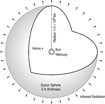
Fig. 1. Diagram of the Sphere. Credit: NASA.
The total solar power that Earth can intercept is estimated to be 1.74×10¹⁷ W, which is roughly the upper-bound for a Type I Kardashev civilization (Zubrin Reference Zubrin1999). Beyond this limit, a civilization on an Earth-like planet would require extraplanetary, space-based power generators (such as a Sphere). This excludes power generation from ‘extelligent’ (Cohen & Stewart Reference Cohen and Stewart2001) systems, such as nuclear power, antimatter and biochemical processes. For this paper, such power generation systems will not be considered.
The purpose of the Sphere is to increase the power available to a civilization beyond the supply of its home planet. Often, the Sphere serves the dual purpose of energy generator and planetoid home to the civilization's inhabitants. However, the construction of the Sphere requires immense material resources – Dyson's original plan for the Sphere was based on a shell 2–3 m thick, with a radius of 1 AU, which roughly comprises the volume of Jupiter.
While the superficial benefits of the Sphere are obvious (primarily, increasing the power capability to ~4×1026 W, 13 orders of magnitude higher than Earth's current energy consumption), there are a number of obvious impracticalities in the design and execution of such a Sphere, as well as numerous, under-appreciated deficiencies that would be created by the Sphere's use.
Impractical materials requirements
If the Sphere is designed so as to receive the same intensity of solar light as Earth (i.e., the radius of the Sphere is 1 AU), then its internal surface area would be
approximately 5.6×10⁸ times the surface area of Earth. Given that there is perhaps 1.82×1026 kg of mass in the Solar System usable for such a project (Sandberg Reference Sandberg2009), that translates into a spherical shell with a mass/unit area of
and
If the Sphere's average density is that of water, it would translate into a sphere just 65 cm thick (see (2b)). If the Sphere's average density is closer to that of steel, the thickness would be closer to 8 cm. These estimates assume that all of the solid and liquid material (at ~100 K; discounting most of the light gaseous material of the outer planets) in the Solar System is used for the project – otherwise, the Sphere becomes far thinner, as the estimated usable material on the inner planets is only ~1/18th of the mass used in (2a). Of course, the primary problem with having such a thin sphere is how such a thin shell would support a civilization on it (since all of the matter of the Solar System has been used to create it).
While there is little structural reason to use a Sphere of such high radius – solar cells can be made to tolerate higher levels of solar intensity – the ability of the Sphere to utilize and/or dissipate heat energy (gained from collision of photons with the solar panelling) is limited by its size. In order to turn heat energy into useful energy, while maintaining a comfortable living temperature within the shell of the Sphere (~300 K), the radius of the Sphere must be ~2.5×10⁸ km, or about 1.66 AU (Badescu Reference Badescu1995). At too small a radius (<2.4×10⁸ km), the efficiency of the Sphere to convert thermal energy into usable energy via a thermodynamic heat engine falls to zero – such a Sphere would eventually store up so much heat energy as to melt/explode. In addition, storing excess heat would cause a breakdown in the potentials of the solar panels, preventing productive collection of solar energy.
Lack of gravitational control
A Sphere concentric around the Sun would experience no net gravitational force due to the Sun (the Sun would pull on it from all directions, netting a vector force of zero). Even if the Sphere were to shift slightly, the net gravitational attraction would still be zero. By the Divergence Theorem
where g⋅dA is the gravitational flux from the star through the closed surface of the Sphere. Because the area of the Sphere is constant and completely closed around the star, the force of gravity is a constant at all points along the Sphere, still resulting in a net vector force of zero. In order to maintain the Sphere around the Sun, then, a complex system of manoeuvring thrusters would have to be employed. Given the mass of the Sphere to be approximately 1.82×1026 kg (ignoring for the time being that a populated Sphere would have to be larger than this), constantly correcting its motion to within a drift speed of only 1 m s−1 would require energy equal to
or about one quarter of the power being absorbed from the Sun in the first place. If correction for a drift speed of just 2 m s−1 were necessary, that would require four times (22) the power in (4), and the purpose of the Sphere would fail to be realized.
In addition, by the Divergence Theorem (3), the gravitational pull of the Sphere on anything inside of the Sphere would be zero (since M sphere inside the spherical shell is zero) – anything on the inner surface of the Sphere would fall straight into the Sun.
Impractical structural stress
Considering the Sphere to be a hemisphere of height equal to 1 AU, the pressure placed on any given seam of the Sphere would be
where F g is the force of gravity, ρ is the density of the materials, τ is the thickness of the Sphere, A shell is the surface area of the shell and A seam is the area of the shell resisting the buckling pressure. Assuming a Sphere of a radius of 1 AU and mass of 1.82×1026 kg, the buckling pressure on any point of the Sphere is
This would translate into a spherical dome on Earth ~85 000 km high. Current technology has not produced a material capable of sustaining such a structural strain. However, it is possible that external vacuum pressure could help to offset this strain to some degree.
Other issues
Building a Sphere to encapsulate the Sun would remove several of the ‘hidden’ benefits the Sun imparts upon its satellites. Foremost amongst these would be the cessation of protections offered by the heliosphere of the Sun: primarily, the ability of the solar wind to deflect the interstellar medium (Fig. 2; Schwenn & Marsch Reference Schwenn and Marsch1991; Linde et al. Reference Linde, Gombosi, Roe, Powell and DeZeeuw1998; Lallement et al. Reference Lallement, Quemerais, Bertaux, Ferron, Koutroump and Pellinen2005). The Sphere would cancel that protection, allowing the gases/plasmas of the interstellar (or intra-galactic) medium to hit the sphere, whittling away at it like a plasmic acid.
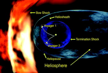
Fig. 2. Picture of the heliosphere repelling the interstellar medium. Credit: NASA.
From the inside, the full force of the solar wind, comprised of a very hot (from 1.4×10⁵ K to 8×10⁵ K) plasma of electrons, protons and light ions, would continuously impact the inner surface of the Sphere (Feldman et al. Reference Feldman, Landi and Schwadron2005). Much like the interstellar medium, although much warmer, it would serve to flay away the surface of the Sphere.
Both the interstellar medium and the solar wind could be diverted via magnetic fields produced by the inhabitants of the Sphere. However, the solar wind constituents would require a constant evacuation to the outside of the Sphere, or the stream of charged particles would build up at a rapid pace.
In addition, sealing the Sun inside a Sphere would eliminate high-frequency light from the star outside of the Sphere (although the shell of the Sphere should increase emissions of infrared (IR) light (Dyson Reference Dyson1960). Even in solar systems with enough matter to form the Sphere without destroying all of the rocky planets, natural, sunlight-dependent life would cease to exist.
A number of varying types of ‘super-structures’ with size and/or purpose similar to that of a Sphere have been proposed by scientists and novelists alike (Sagan Reference Sagan1973; Niven Reference Niven1974; Badescu & Cathcart Reference Badescu and Cathcart2000). Perhaps the most realistic variant would be the Dyson Swarm (Sandberg Reference Sandberg2009): a collection of solar sail satellites in orbit around a star, which would have the purpose of collecting solar energy. The benefits of such a system are many: a large number of satellites can be made without requiring large amounts of materials, even multitudes of such satellites would not significantly impact the output of the star, and current technology would allow for their construction.
Of course, the disadvantages are numerous too: the satellite system would provide only a fraction of the Sun's energy for a civilization's use, satellite systems would require complex orbital and manoeuvring systems, and the energy they collect would need to be redirected and/or stored for later use.
The Solar Wind Power Satellite
As an alternative to a traditional Sphere, we propose the design of a Dyson-like satellite called ‘SWP Satellite’ (or hereafter simply ‘satellite’), which would utilize the energy of the solar wind rather than photonic energy. Primarily, the benefits of the SWP satellite would be: (1) protection from solar wind decay; (2) absorption of minimal heat; (3) a self-sustaining apparatus requiring little upkeep, even over the variances of the solar wind cycles; (4) nearly 100% efficiency; (5) laser-directed power output to distant satellites, space stations or planetary installations; and (6) the use of innately super-cooled metals would prove less sensitive to aging or extreme effects than the relatively delicate systems of solar panels. The SWP Satellite would be a device that could be easily constructed with current technology, and could draw off vast amounts of energy from the solar wind. The design of the SWP Satellite is shown in Fig. 3.

Fig. 3. The design of the SWP Satellite. The Sun (A) emits a plasma, half composed of electrons, half of protons and positive ions (B) (Encrenaz et al. Reference Encrenaz, Bibring and Blanc2003). Electrons are diverted (via Lorentz force from a cylindrical magnetic field (C)) from their radial trajectory towards the ‘receiver’ (D), a metallic spherical shell. Note that when the receiver is ‘full’, excess electrons are diverted through the hole in the ‘sail’ (G). The large positive potential on the sail drives an electron current through the ‘pre-wire’ (E), which is a long wire, away from SWPS, to remove its magnetic field from the local area of the main wire. Once it reaches the end of the pre-wire, it travels down the ‘main wire’ (F), creating the magnetic field (C), which makes the self-sustaining field-current system. The current passes through a hole in the receiver and then through the sail (G), passing through the ‘inductor’ (H), and the ‘resistor’ (I), which draws off all of the electrical power of the satellite to the ‘laser’ (J), which fires the electrical-turned-photonic energy off to a designated target. Drained of its electrical energy, the current continues to ‘fall’ to the sail (G). Here, electrons will stay until hit by appropriately energetic photons from the Sun, at which point they will leap off (K) the sail towards the Sun, and then are repelled by the magnetic fields (C) and excess the Solar wind electrons (B) away from the satellite, imparting kinetic energy to the satellite away from the Sun.
Collection of solar wind particles
The surface of the Sun consists of a plasma in which temperatures average over 106 °C (Encrenaz et al. Reference Encrenaz, Bibring and Blanc2003). This thermal energy grants the particles contained therein an average velocity of ~145 km s−1, not quite the escape velocity of the Sun (~618 km s−1). However, a portion of the particles gain enough thermo-statistical energy to escape the corona via a terminal velocity of ~400 km s−1 – this collection of particles makes up the ‘slow’ solar wind, which is released in the solar plane (the plane formed by the Sun and the planets) at an angular spread of ~±20° (Fig. 4).

Fig. 4. The angular spread of the Solar wind components. Credit: NASA.
However, the slow wind is highly variable and more susceptible to solar flares or other irregularities (Meyer-Vernet Reference Meyer-Vernet2007), making it unfavourable for the purpose of continuous energy absorption. The fast solar wind, on the other hand, has a fairly constant flux, and a velocity of ~750 km s−1 (Maksimovic et al. Reference Maksimovic2005; Meyer-Vernet Reference Meyer-Vernet2007). The fast wind is dominant at more than ±30° from the solar plane, so placing the SWP Satellite in an almost perpendicular orbit to the solar plane not only allows collection of fast wind particles, but it would also give the satellite continuous sight to all of the planets, important for not blocking the laser beam that diverts power to other parts of the Solar System.
The total number of particles lost by the Sun via the solar wind is ~1.3×1036 particles/second. Approximately half of those are protons and ions (all ions emitted by the solar wind are positively charged; Kallenrode Reference Kallenrode2004). We will use this figure to determine the flux of electrons that can be absorbed by a SWP Satellite. While the kinetic energy of these electrons is high (2.56×10⁻¹⁹ J≈1.6 eV), their high velocity will be used to increase the magnetic force the satellite can apply to them, and to increase the number of electrons that can get onto the receiver before the net potential of the receiver starts pushing incoming electrons away. A consistent flux of electrons will create a consistent potential on the receiver, ensuring a constant current through the satellite, and therefore a constant energy stream from the satellite's laser.
Charge collection (un)limitations
The current of electrons from the solar wind collected by the receiver is technically limited by the potential that can start repelling incoming electrons. To determine this, we apply conservation of energy considerations as follows:
where m=9.11×10⁻³¹ kg, v≈750 km s−1, k=1/(4πε0)=8.99×109 N⋅m2 C−2, q=1.60×10⁻¹⁹ C, Q is the charge on the receiver and r is the radius of the receiver (Fig. 3). If we assume r=1 m, the maximum charge that can be built up on the receiver is only ≈1.78×10⁻¹⁰ C. If this were cycled through the circuit every second by assuming that the solar wind could place a maximum of Q on the receiver per second, then the resulting r B,max would be about 3.7 cm – enough to divert the needed charge from the solar wind onto the receiver, but not enough to protect the sail from the rest of the solar wind.
This apparent deficiency can be solved in two different ways: superconductivity or capacitance. If a superconducting material (say, aluminium) is used to create the SWP Satellite, then the charge is conducted away from the receiver to the sail (which has a very high, positive potential) rapidly – perhaps not as rapidly as, say, 750 km s−1, but rapidly enough so as to assume the limiting current is not based on the charge build-up on the receiver.
Another method of tackling this issue is to create a capacitor from the receiver by lining the interior with dielectric material, then attaching another sphere, which is held at the potential of the sail (see Fig. 5). This could allow the build-up of much more charge onto the receiver, while allowing both the voltage and the resistance of the circuit to be user-defined parameters, the former by the potential difference between the capacitor and the latter by using a non-superconducting material in the satellite (e.g., copper). The following discussion assumes this style of design.

Fig. 5. A capacitor-style receiver. This is a close-up, transparent view of a receiver that is filled with dielectric material, in order to increase the capacitance of the receiver to increase the charge it can collect from the solar wind.
The photoelectric effect and laser power
Briefly, the photoelectric effect is the phenomenon by which an electron is ‘pushed’ free from the surface of a metal via absorption of a sufficiently high-energy photon. The process occurs discretely if the photon's energy is sufficiently high, which is based on the metal's physical properties, its temperature and the electric potential at which it is held. Essentially, the current (of electrons) that the photons from the Sun can pull off of the sail is
where N γ* is the number of photons from the Sun with energies equal to or higher than the energy required to eject an electron from a metal's surface, A is Richardson's constant for thermionic emissions (1.20×10⁶ A m−2⋅K2), T is the temperature of the metal, W is the work-function of the metal (i.e., the metal's intrinsic ability to hold onto free electrons), and k B is Boltzmann's constant (1.381×10⁻²³ J K−1) (Ashcroft & Mermin Reference Ashcroft and Mermin1976).
Note that for low temperatures – the equilibrium temperature of a spacecraft at 1 AU is ~280 K (Juhasz Reference Juhasz2000) – the thermionic emission (the exponential term in (8)) is minimal. However, at higher temperatures, emissions of electrons due to heat can become significant.
The design and operation of lasers is fairly inconsequential for the purposes of studying the SWP Satellite; simply choosing a laser with an appropriate emission frequency and pump energy would suffice. The important concept for the laser's operation in the satellite is that it can be used to funnel energy (electrical and heat) from the satellite into space.
SWP Satellite parameters
Where there are moving particles, there is energy: kinetic and electric. The SWP Satellite utilizes the former to divert the path of electrons onto the receiver, and the latter to both maintain the satellite's magnetic field as well as to power the laser and provide useful energy.
However, the calculations become complicated quickly as one begins to analytically approach the problem. Firstly, if the collection of electrons is too fast at the receiver, then the receiver eventually will reach a potential energy strong enough to push away incoming electrons. In addition, the potential of the sail will be the upper bound of the satellite's total potential, resulting in a current through the satellite of
where V max and V sail are given by the potential at which the receiver has enough potential energy to repel incoming electrons (9b), and the ability of the photoelectric effect to rip electrons off of the sail (9c), respectively:
and
where q e is the charge of an electron, m e is the mass of an electron, v wind is the velocity of the incoming electron, V T is the potential difference through the satellite and I photo is the current pulled off of the sail via the photoelectric effect. Note that using a capacitor receiver as pointed out previously allows V T to be tuned by design, in terms of V sail.
To identify the limiting effect on the system – the satellite's ability to pull electrons onto the receiver, or the Sun's ability to pull electrons off of the sail – the relative fluxes of particles and photons must be found.
The Sun emits 3.85×1026 W of power via photons, 7% of which have frequencies in the ultraviolet (UV) or higher spectra. This is important if the sail is composed primarily of copper (W≈4.8 eV; λphoto⩽258 nm) or aluminium (W≈4.1 eV; λphoto⩽303 nm). The number of super-visible (‘UV+’) photons the Sun emits is therefore
where P UV is the power emitted by the Sun in the UV or higher spectrum, N γ* is the number of UV+ photons/sec from the Sun, h is Plank's constant (6.626×10⁻³⁴ J⋅s−1), c is the speed of light (3.00×10⁸ m s−1) and λmed is the median wavelength of the UV spectrum, 300 nm. Note that the Sun's UV+ spectrum is made up of photons with wavelengths that are different from 300 nm, and therefore N γ* is an upper-bound limit on the number of photoelectrically useful photons that can be gathered from the Sun. The number of photons that hit the sail is
Clearly, the size of the sail (A S) defines the total number of UV+ photons actually available to the satellite. Similarly, the size of the satellite's magnetic field determines the number of electrons it can receive, through the equation
where N e−,R is the number of electrons r B,maxcould receive, provided the total charge build-up on the receiver is not so high as to repel high-velocity electrons; N e−,S is the number of electrons emitted by the Sun, estimated to be ~6.5×1035 electrons/sec; and r B,max is the maximal radius at which the satellite's magnetic field can drive electrons to the receiver via the Lorentz force. The area terms represent the fraction of the electron flux going through the satellite's maximum capture area (MCA=π⋅r B,max2), which in turn is governed by the current through it as follows:
where B is the magnetic field at a distance r perpendicular to the main wire, μ0 is the permeability of free space (4π×10−7 N A−2) and I is the current through the satellite. r B,max is now determined by the solving the following equation:
where r final is the main wire (set as the origin of this coordinate system), a=F/m is the acceleration an electron is exposed to from the time it is parallel to the main wire to the time it either passes the wire or is received, F is the Lorentz force on the electron (F=qv×B), q is the charge of an electron (1.60×10⁻¹⁹ C), v is the velocity of the electron (~750 km s−1), and t is the time the electron is parallel to the wire (and therefore the time it is subject to the magnetic field), starting at t=0 when it first passes the wire's sunward tip. If l M is the length of the main wire, then t=l M/750 km s−1. Analytically, r B,max is given by
To find r B,max numerically, the desired current through the satellite must be determined, recognizing that the density of the solar wind is far higher than any desirable current – a current of 1 MA (mega-amps) from the solar wind only requires an r B,max of 0.19 mm to collect it. The satellite relies on the repulsive abilities of a fully charged receiver to deflect solar wind electrons that are not needed for the satellite's operation, just as it relies on the main wire's magnetic field to deflect positive ions away from the sail.
Figure 6(a) shows what the path of an electron looks like when it is subject to the satellite's magnetic field at r B,max, Fig. 6(b) shows the path the electron follows if it enters the MCA at r<r B,max and Fig. 6(c) shows the path of the electron as it nears the satellite, but at distances outside of the MCA. Note that if the electron is close to the main wire, its path is oscillatory, and eventually ends up on the receiver. Figure 6 was created based on (11c), although since force is not constant it was solved numerically.
Note that the pre-wire shares the same magnetic profile as the main wire, except that it repels electrons. Although this effectively doubles the amount of solar wind diverted (see Construction…, below), its distant magnetic effects near the main wire have not been considered.

Fig. 6. The schematic paths of an electron are shown for (a) r=r B,max, (b) r<r B,max, (c) r >r B,max. Extra distance is in (c) to show the lack of force applied to the electron once it passes the main wire.
To determine what the limiting factor or better, predetermined current limit is, compare (10b) and (11a):

If l M is 100 m, I=100 A ((11d)→r B,max=150 m) and A S=100 π m2, then the ratio in (12) is ≈2100. For these parameters, the sail's ability to lose electrons to the Sun's UV+ photons is much higher than the solar wind's ability to put electrons onto the receiver. The latter, however, is further limited by the charge build-up of the pre-set receiver capacitance; the solar wind could deliver 2.89×10¹⁵ electrons/sec onto a receiver at the heart of a magnetic field with r B,max=10 m. Therefore, the desired current through the satellite is solely determined by its engineering, and not by the limitations of the Sun to provide energetic particles or photons.
Parameters for useful power
Given the ring-like sail parameters of R S=3 m (inner edge) and 10 m (outer edge), thickness, τ=1 mm, and the separation distance between the sail and the receiver of (3 m – 1 m) 2 m, the free electrons lost from the sail via UV+ photons totals
where ρCu is the density of free electrons in copper (13.6×10⁹ C m−3). In (13a) we assumed that the UV+ photons can completely strip the sail of its free electrons. This translates into a potential difference between the receiver and the sail of
assuming that the charge build-up on the receiver creates a negative (by sign conventions) potential of only about −1.6 V. Intuitively, this is ‘too high’, and does not take into account the inability of electrons to escape from the sail in the presence of such a high positive potential. However, the receiver cannot hold all of the electrons that the magnetic field can acquire, resulting in a net flow of electrons through the centre of the sail. Electrons ejected from the edges of the sail via the constant stream of UV+ photons will be pushed away by the remnants of the solar wind; hence, r B,max should be equal to 10 m (from (11d), this makes I=0.444 A). The lateral distance from which an electron can escape from the sail is based upon the potential of the sail and the energy of the photons as follows:
This is the initial velocity with which the electron is ejected from the sail by a photon of λ=200 nm. The distance from the (inner) edge from which an ejected electron can use the magnetic field to escape the radius of the sail is found by approximating a constant magnetic force as follows:
The time that the electron remains off of the sail (i.e., the time it would take for the electron to ‘fall’ back to the sail in the absence of a magnetic force) is (approximating a constant, maximal potential on the sail)

Inserting (13e) into (13d), and assuming that r min≈100 pm (approximating that the photon ejects the electron starting at a distance roughly equal to the radius of a nucleus), we obtain
This is the distance from the outer edge of the sail for which electrons ejected by UV+ photons can be forced outside of the radius of r B,max=10 m by the magnetic field, and therefore swallowed by remnants of the solar wind before they come crashing back into the sail. Incidentally, this also sets the minimal size of the sail. Now, the free electrons hit by UV+ photons at the edge of the sail and released can be determined (repeating (13a) for new A S) as follows:
which makes the effective potential of the sail (repeating (13b), for a separation distance between the sail and the receiver of 2 m),
Note that this potential has not accounted for subtle magnetohydrodynamic forces, and may overestimate the amount of electrons that can be photoelectrically removed from the sail.
The current through the SWP Satellite was engineered to be 0.444 A (to make r B,max=10 m). If the length of the satellite's circuit is ~300 m of copper wire, the joule-heating resistance is
where ρR is the resistivity of copper wire, l is the length of the total wire in the circuit, C is the temperature coefficient of copper (Griffiths Reference Griffiths1999) and T is the circuit's temperature (Juhasz Reference Juhasz2000). The power lost to joule heating is ~3.88×10⁻³ W, which means the useful power available to the satellite's laser is (P=VI)~1.7 MW.
The amount of 1.7 MW is useful for about 1000 single-family American homes, and can provide about 52 times the power generated by the International Space Station (ISS) (~32.8 kW peak DC power). However, because I is a user-defined parameter (by the choice of r B,max), changing I can alter the useful power garnered from the solar wind. For example, doubling the current through the satellite increases the potential in (14b) to ~5.3 MV, which gives a useful power of ~4.78 MW. Figure 7 shows a graph of how increasing the current affects the power output by the satellite. Note that power varies with the square of the current.

Fig. 7. Power generated by the SWP satellite as a function of current through the satellite.
For the treatment of finding useful power generation we have utilized a constant force approximation. To be more precise, partial differential equations must be solved or numerically modelled. This would show an increase in the useful power generated by the satellite, since forces here were chosen to determine the lower bound for generated power.
Solar pressure and photoelectric kinetic energy
The temperature of the satellite is important in order to maintain a low resistivity through all parts of the circuit except the laser, as well as to ensure that the satellite does not melt. There are three sources of heat in the satellite.
(a) Power loss by Joule heating as the current travels through the satellite's wires. However, provided the current temperature is low, the current must exceed 260 A to begin to produce 1 W of heat (see (14c)).
(b) Solar wind particles are one of two sources of heat for bodies exposed to them. However, the satellite is designed to divert most of the solar wind particles away from it, including the heavier positive ions that have more kinetic energy. Of the particles that actually land on the receiver, they are few in number, and are low in kinetic energy, and therefore are not the limiting factor in the determination of temperature.
(c) The photons that strike the sail (including ones with lower energy) add the most significant contribution to the satellite's temperature.
To minimize the effects of temperature on the SWP Satellite, it can lose heat to electrons that are successfully ejected from the sail, it can lose heat to black-body radiation or it can utilize a heat laser, which generates laser energy based on the excitation of phonons (vibrational states) rather than electronic states (Yariv Reference Yariv1989) How much energy does the satellite need to be able to dissipate? The satellite is hit with ~1.71×10⁶ W of photonic power (P in), most of which are the lower frequencies that are not helpful for photoelectrical electron ejection. The volumetric heat capacity of copper is 3.45 J cm−3⋅K (C in (15), below) (Tipler Reference Tipler1999). If the satellite's volume (Vol) is roughly approximated as 410 000 cm3 of copper, then the Sun's photons warm the satellite to
which is less than 1% of the satellite's expected equilibrium temperature of ~280 K. Assuming the satellite can dissipate ~1.2 K s−1 of heat, it should remain at a constant temperature. Concerns of excess heat build-up are minimal. Coincidentally, the critical temperature for superconductivity in aluminium is 1.2 K (Cochran & Mapother Reference Cochran and Mapother1958). If the equilibrium temperature of the satellite could be lowered, it might be possible to use superconductive effects in an alternate design.
Another concern is the gravitational stability of the SWP Satellite imparted by the solar wind. Given that the density of copper is 8.960 g cm−3 and the estimated volume of the satellite is 410 000 cm3, the total mass of the satellite is approximately 3700 kg, which makes the gravitational force on the satellite
The Solar pressure exerted on the Sail at R O=1 AU is only 1×10⁻⁵ Pa, which is only ~0.003 N of force onto the satellite. However, the kinetic energy imparted onto the satellite by the photoelectrical ejection of electrons is given by the energy that the electrons are granted by photons in the sunward direction, and by the energy with which the majority of those electrons impact back into the sail. The number of electrons ejected by UV+ photons is given by
With these electrons ejecting at v 0=1.48×10⁶ m s−1 (see (13c)), the force imparted by the electrons is the momentum imparted over time as follows:
where p is the momentum of the electrons and t is given by (13e). This is far too low to achieve gravitational stability, which would be valuable for maintaining a steady aiming mechanism, as well as for easing the calculations for firing off the laser.
Analysis
The SWP Satellite has a number of advantages for pursuing it as an astro-engineering project. The design proposed herein is beneficial: it should have minimal heat issues; it can create a lot of power that can be sent off via laser to energy collectors around the Solar System at virtually 100% efficiency; the lasers required for the satellite can be built with current technology; being posted in the region of the fast solar wind means the satellite does not affect the light from the Sun to the planets; a single small satellite only diverts 4.44×10⁻¹³% of the solar wind, most of which gets reintegrated into the solar wind, slowing the wind by less than one trillionth of its initial energy. Finally, the satellite (minus laser) should be relatively cheap to construct based on the inexpensive materials needed for construction.
While the satellite as proposed is very advantageous, it has a few critical weaknesses, which may need to be addressed before the satellite can be used efficiently. Compared to the grand design of the Sphere, the SWP Satellite has a relatively low power output. Whilst the satellite may be a good choice for humanity's foray into extraterrestrial habitation, it is not a feasible option for a truly advanced civilization's power needs. However, it can easily be scaled up.
The satellite, while designed to require as little upkeep as possible, is not self-cleaning: when positive ions (of particularly high velocities) get caught in the sail, there currently exists no mechanism to ‘clean’ them off. It cannot maintain a steady location in space, which would serve to complicate the aiming calculations, as well as require that the satellite spend some time in the slow solar wind region. In addition, while the satellite can maintain its current (and therefore its r B,max) via capacitor systems and the inductor that prevents temporary swings in current, the current system needs to be started manually. It is possible that the system can self-start, but this would require more complex numerical modelling to demonstrate, as well as require more complexity of the launch vehicle.
Finally, creating a small-scale, high-power laser may prove difficult. While high-power laser systems can be built with current technology, they are still large-scale endeavours.
Construction and remote detection of Solar Wind Power Satellites
Scientific missions designed to find Spheres – thereby finding proof positive of intelligent, space-faring life – are not uncommon (Dyson Reference Dyson1960, Zubrin Reference Zubrin1999). More recently, there has been an increased interest in searching the skies for astro-engineering projects and other evidence of advanced civilizations (Tough Reference Tough2000). Thus, there are obvious astrobiological interests related to the construction and discovery of SWP Satellites.
We assumed a very basic design for the SWP Satellite, which minimizes the complexity of the system for the sake of long-term autonomy and cost effectiveness (Table 1). Most materials/components for the construction of the SWP Satellite would be feasible to assemble. The trickiest part of the design process would likely involve the laser system. The laser itself would be fairly straightforward to design and construct: any optically/magnetically pumped pulse laser or, perhaps preferably, maser with decent heat dissipation would do. However, the size of the laser is a critical design issue. Additional complexity would arise in the system used to aim the laser, which at the very least would require a small satellite receiver dish (to receive instruction/correction signals), a digital logic circuit board (for processing inputs) and electromagnetic servos (for tweaking the aim).
Table 1. Describing the construction characteristics of a 1.7 MW SWP Satellite

‘ TBD’=to be determined.
Of course, the SWP Satellite is not of much use without collectors that receive the satellite's energy for powering an Earth base, lunar base, Mars base, or space station, to which the collector is connected. Depending on the complexity of the laser system, a collector may need a feedback component that uses a small part of the collected energy to send back to the satellite a signal with information regarding drift. A simple collector might consist of a large, basic satellite dish, although a collector with a feedback system could cost much more, and would require more complex construction.
While as a global civilization we may not yet need power-generating satellites for our energy needs, the prospect of finding existing astro-engineering projects as proof of intelligent, technologically advanced extraterrestrial life is clearly an astrobiological objective.
Unfortunately, current technology can only detect solar winds and alterations to them of the order of ~3×10⁻¹³ MS yr−1, where MS is the solar mass (Wargelin & Drake Reference Wargelin and Drake2002). The Sun loses a total of ~2×10⁻¹⁴ MS yr−1 in the form of its solar wind. The proposed SWP Satellite would divert ~8×10⁻²¹ MS yr−1 of the local solar wind – not absorb, just divert. Far from the satellite, it is questionable whether the diversion can even been seen, as the diverted particles simply get swept away by the bulk remainder of the wind. In fact, if the wind is approximated as a plasma gas, then the diffusion time is
where t is the time required for the wind to re-equilibrate itself, L is the length over which it must do so (assume roughly twice r B,max) and D is the diffusion constant for the solar wind plasma (Ruffolo et al. Reference Ruffolo, Matthaeus and Chuychai2003). Given that the velocity of the fast solar wind is ~750 km s−1, the wind travels only ~1.67×10⁻¹⁴ m in that time – unintuitively small. Given a diffusive process over long time scales, clearly the deviation distance must approach AU in order to carry the deviated pattern any significant distance. Such a satellite might have an r B,max of ~0.5 AU, which would divert up to 25% of the solar wind, and would be detectable if the X-ray methods used by Wargelin & Drake (Reference Wargelin and Drake2002) become about 10 times more precise (incidentally, such a satellite would theoretically produce of the order of 1×1027 W of power – assuming a main wire length of 1 km and a sail with an outer radius of 4.2 km – almost 3.5 times that of a Sphere around the Sun (Phillips Reference Phillips1995)).
Conclusion
The Sphere has long been a hallmark of science fiction media, despite its original conception as a serious proposal for IR telescopic missions. While the power it could generate – by definition, the power output of an entire star – is great, so too are the engineering challenges one would need to surmount to build it.
Dyson variants comprise various wire and satellite networks designed to recover a fraction of the power an entire Sphere could collect. Here we propose as one of these variants the SWP Satellite, which collects energy from the solar wind instead of the Sun's light (although it does utilize some of the high-energy light to ‘complete’ the circuit). The benefits of that type of satellite are many – it is self-sustaining, inexpensive, and can collect large amounts of power – while it's only real deficiency is the same shared by all Dyson systems – once it has the energy, what does the satellite do with it? The SWP Satellite would fire the energy to projects in need of power (space stations, bases on planets or moons, etc.) across the Solar System.
A small satellite might only be able to provide ~2 MW of power, requiring more than 7 million such Satellites to satisfy the energy needs of Earth's modern population. Although, a much larger satellite with a main wire 1 km long and a sail with an outer radius of 4200 m could easily supply the entirety of humanity's power needs. Initially however, SWP Satellites may find their niche in serving as dedicated power sources for individual space-based projects – one may be used to power a lunar base, another to power a space station, etc. SWP Satellites cannot be found with current detection methods, but an increase in size will increase the chance of detection as might further advances in technology.


