Dynamical system and initial conditions

We have assumed a hypothetical triple system of stars whose orbital parameters and masses are similar to the system HD98800. In our model the triple system is composed by an internal binary (Ba and Bb) orbited by a protoplanetary disc and a distant star (A). Evidently, as mentioned before, there is a wide range of parameters of the system to explore. Here we have focused on exploring the consequences of considering different orbital inclination for the disturbing star. Thus, we have used a single set of values for the masses and orbits of the inner binaries, and also for the mass of the third star.

The stars Ba and Bb have 0.699 and 0.582 solar masses, respectively. Their semi-major axes with respect to the centre of mass of the binary are a _Ba=0.447 AU and a _Bb=0.536 AU, and the orbits have eccentricity equal to 0.7849 (Boden et al. Reference Boden, Sargent, Akeson, Carpenter, Torres, Latham, Soderblom, Nelam, Franz and Wasserman2005). The orbit of the A star was placed around the centre of mass of the B pair. The mass of the A star is the sum of the masses of the inner binary (M _A=1.281 solar masses) and its orbital parameters are a _A=61.9 AU, e _A=0.3, Ω_A=184.8° and ω _A=210.7° (Tokovinin Reference Tokovinin1999). We have performed simulations considering different values for the orbital inclination of A star. The initial inclinations of A star (I _A) are given with respect to the initial B binary plane and are taken in the range from 0° to 50°. The values initially assumed were 0.0°, 0.01°, 0.5°, 2°, 5°, 10°, 30° and 50°.

For the hypothetical triple system here considered, Domingos et al. (Reference Domingos, Winter and Carruba2012) who numerically obtained a region in a semi-major axes and eccentricity distribution (a, e) for which particles could survive for long timescales around the centre of mass of the inner binary; see Fig. 1. The results showed that, in general, particles can survive longer when they are initially in the range of ~3.4–12 AU and when the stars are initially in coplanar orbits. However, n : 1 mean motion resonances with inner binary and third star, respectively, overlap some regions of this stable region creating gaps in the distribution of particles. Using the semi-empirical formulas of Holman & Wiegert (Reference Holman and Wiegert1999), we found the stable region to be between ~4.04 and 11 AU. These boundaries are very close to those found in the numerical study by Domingos et al. (Reference Domingos, Winter and Carruba2012).

Fig. 1. Region of stability of the particles in the space of a versus e for the coplanar case (I _A=i=0). The stable region is delimited by red and green lines. The red and green lines represent the internal critical semi-major axes, a _I, and the outer critical semi-major axes a _O, respectively. The dashed line represents the limit eccentricity, e _lim, for a particle within the stable region (Domingos et al. Reference Domingos, Winter and Carruba2012).

Figure 1 shows numerical results of the final eccentricity as a function of the final semi-major axis of the particles after 1 Myr of integration. The stars are considered in coplanar orbits. The region is delimited by red and green lines that are obtained from empirical expressions which provide the inner and outer edges of the stable region (for more details see Domingos et al. Reference Domingos, Winter and Carruba2012). While test particles are ‘inside this region’ they keep stable orbits, i.e. they are neither ejected from the system nor collide with the stars. The limit eccentricity, e _lim, shown in this figure is a reference value for the maximum eccentricity in which the orbit of a test particle is still located inside the stable region (region delimited by red and green lines). The value of e _lim is approximately 0.572.

For the cases of inclined orbits, when the initial relative inclination between the particle and the A star i _rel⩾40°, three distinct structures are defined and located on the disc: (i) a chaotic region that is close to the inner binary, (ii) a stable region where particles on highly inclined orbits can survive and (iii) an unstable region that depends on the distance of the third star and the relative inclination of the particles. Depending on the initial conditions of the third star and the disc particle, eccentricity peaks and gaps might appear within the stable region.

It is interesting to note that in the system studied here, the Kozai–Lidov mechanism (Kozai Reference Kozai1962; Lidov Reference Lidov1962) indeed takes effect on the circumbinary disc when the relative inclination of the particle and third star orbital planes is greater than 40°. However, as Verrier & Evans (Reference Verrier and Evans2009) showed the inner binary may cause a nodal libration instead of Kozai–Lidov cycles, which stabilizes the test particles orbits against any Kozai–Lidov instability driven by the outer star. These authors reported that particles closer to the inner binary have nodal libration periods shorter than Kozai–Lidov cycles. Therefore, the nodal libration tends to dominate, which results in a stable region. Otherwise, when particles are more distant, closer to the outer border of the stability region, they tend to have Kozai–Lidov periods shorter than the nodal libration, thus, they are usually destabilized and are ejected from the system or collide with the inner binary.

In our simulations of planet formation, we have assumed that the growth of dust grains and planetesimals during the early phases of planetary accretion were successful and resulted in the formation of a disc of protoplanetary bodies with masses ranging from Moon to Mars-sized objects (Kokubo & Ida Reference Kokubo and Ida2000). In our simulations, the protoplanetary disc extends from 6 to ~8 AU. The choice of this region is justified by the results presented in Domingos et al. (Reference Domingos, Winter and Carruba2012) (Fig. 1). That work has shown that, for the hierarchical system here studied, there is a stable region between 3.4 and 12 AU, where test particles could survive for long timescales. However, some subregions in this stable area are overlapped by n:1 mean motion resonances with the inner binary or with the third star that disturbs and tend to scatter out of the system many bodies, creating gaps in the disc (Domingos et al. Reference Domingos, Winter and Carruba2012). As the main goal of our study is to present the effects of a third star inclination on the formation of planets around an inner binary, we have distributed our protoplanetary bodies in a central narrow region from 6 to 8 AU, located inside the part of the region between 3.4 and 12 AU where strong mean motion resonances do not exist and consequently gaps are not created.

The protoplanetary bodies of our disc are initially distributed around the centre of mass of binary B. The initial mass distribution of the circumbinary disc chosen in our model is based on values calculated according to the Minimum Mass Solar Nebula (hereafter, MMSN; Hayashi Reference Hayashi1981). However, as the amount of mass in protoplanetary discs around binary and multi-stellar systems are poorly constrained, we have also performed simulations considering discs with different amounts of mass. In these cases we adopted amounts of mass proportional to 0.5, 1, 2 and 4 times the value expected in models of MMSN, for a region between 6 and 8 AU. The body size distribution used in our simulations is similar to that used in Chambers (Reference Chambers2001) and Quintana & Lissauer (Reference Quintana and Lissauer2006). For the disc model proportional to 0.5×MMSN, 140 lunar-sized planetary embryos of mass m=0.00933 M _⊕ (2.8×10⁻⁸ M _⊕) were randomly distributed from 6.05 to 8.05 AU. Other 14 Mars-sized planetary embryos of mass M=0.0933 M _⊕ (2.8×10⁻⁷ M _⊙), were equally spaced in the range of 6.0–8.0 AU, giving a total mass of ~2.6 M _⊕, which corresponds to a separation between embryos in the range between 3 and 6 mutual Hill radius. This is compatible with Runaway and Oligarchic models of planet formation (Kokubo & Ida Reference Kokubo and Ida1998, Reference Kokubo and Ida2000). For higher-mass discs we have, for simplicity, increased the number of lunar-sized and Mars-sized planetary embryos distributed in the disc according to the factor that the disc mass has been increased. For example, for a disc with a mass proportional to 1×MMSN, we doubled the number of bodies to 280 lunar-sized planetary embryos with mass m=0.00933 M _⊕ 2.8×10⁻⁸ (M _⊙) and 28 Mars-sized planetary embryos with mass M=0.0933 M _⊕ (2.8×10⁻⁷ M _⊙), giving a total mass of ~5.2 M _⊕ distributed between 6 and 8 AU. In our simulations, all bodies were assumed to have a bulk density equal to 3 g/cm³. Bodies of the disc have initial eccentricities raging from 0 e to 0.01 and initial inclinations i=0°. The other orbital elements were randomly distributed.

All simulations were numerically integrated for at least up to 10 million years. Collisions between planetary embryos are considered inelastic such that in each collision mass and linear momentum are conserved and a new body is formed. A body is considered to be a planet when it has M _P⩾0.3 Earth-mass (M _⊕). The integrations were performed using the package of numerical integration MERCURY (Chambers Reference Chambers1999). We used the Bulirsch–Stoer integrator (Press et al. Reference Press, Teukolsky, Vetterling and Flannery1996) with an initial time step of 3 days.

Results and discussion

Our numerical results are summarized in Figs 2–6, which refer to the final orbital evolution of the particles on the a–e and a–i planes. In order to study the coplanar regime (I _A=i=0), we conducted experiments considering protoplanetary discs carrying different amounts of mass. Table 1 shows the final results.

Table 1. Mass and final orbital parameters of the planets formed, continued

Coplanar orbits

We have performed a total of 60 numerical integrations considering the coplanar regime. For each disc model (e.g. 1×MMSN), a total of 15 experiments were carried out with slightly different initial configurations for planetary embryos. Since the CPU time to run these simulations is relatively short, we integrated them for 10⁸ years.

Tables 1 and 2 present a summary of the final results of all our numerical simulations for the coplanar cases. The columns are the simulation, the initial mass of the protoplanetary disc, the number (N) of planets formed whose final mass M _p≳03 M _⊕, the final mass M _P of the planet, the final semi-major axis a _f (AU) of each planet, the final eccentricity e _f of the planet and the time T (Myr) of the last ejection and/or collision of protoplanets during the integration period.

Table 2. Mass and final orbital parameters of the planets formed, continued

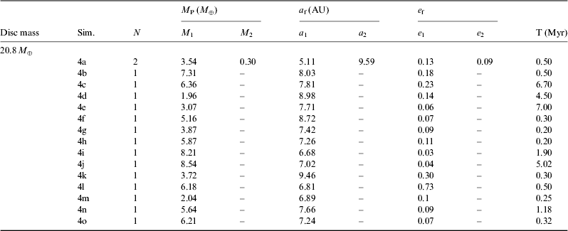
Figure 2 shows snapshots of two representative results of our simulations. In these cases the protoplanetary discs carry initially 2.6 M _⊕. The dynamical configuration of the planetary embryos are shown by snapshots at times 10⁴, 10⁵, 5×10⁵, 10⁶ and 10⁷ years. The mass and orbital elements of the final bodies stayed almost unchanged after this time. We can note that after 10⁴ years the eccentricity of the planetary embryos increase significantly. Such increase is due to the mutual interaction among the objects in the disc. This orbital excitation results in the crossing of orbits of objects of the disc, leading to successive collisions and the formation of planets. For example, in Fig. 2, after 10⁵ years it is possible to note the formation of the first protoplanets in the system. These more massive bodies have accreted very quickly between 2 and 5 times the amount of their initial masses. Note that in 10⁵ years, bodies with masses between 0.3 and 0.6 M _⊕ already have been formed inside a region between ~6 and ~8 AU. As shown in Fig. 2, the eccentricities of these massive bodies are smaller than 0.1, while lunar-sized planetary embryos evolve to more eccentric orbits, due to their interaction with Mars-sized planetary embryos. The process of planetary accretion slows down as the amount of mass available for accretion in the system decreases. In both simulations, after 0.5 Myr of integration the process of planetary growth has ceased almost completely and we note the formation of two potential planets in each system. However, extending the numerical integration up to 10 Myr, in the left-side simulation formed two planets with masses equal to 0.82 M _⊕ (8.74 AU) and 1.17 M _⊕ (6.60 AU), while that in the right-side plots only one planet with mass equal to 1.91 M _⊕ at 6.76 AU survives. Tables 1 and 2 summarize the final results of our simulations within the coplanar case after 10⁸ years of integration.

Fig. 2. Snapshots of the formation and dynamical evolution of planets in 1a and 1l simulations shown in Table 1 (initial mass of the disc equal to 2.6 M _⊕). In both experiments all stars and the protoplanetary disc are in the same orbital plane (I _A=i=0). In the left-hand plot (1a case), we note the formation of two planets with masses 0.82 M _⊕ (8.74 AU) and 1.17 M _⊕ (6.60 AU) in less than 0.5 Myr with low eccentricity orbits. Only one lunar-sized embryo survives in case system for 10 Myr, the other are ejected from the system or accreted by the planets. In the right-hand plot (1b case) has been formed only one planet with mass equal to 1.91 M _⊕ at 6.76 AU. These simulations were integrated numerically for 10⁸ years.

Figure 3 shows the final distribution of planets in M _P–e (top) and a–M _P (bottom) diagrams for all the simulations with disc mass of 2.6 M _⊕. Recall that the initial distribution of bodies in the protoplanetary disc extend from 6 to 8 AU. Thus, as expected, there is a concentration of planets formed inside this region. The bigger planets (0.8–2.1 M _⊕) formed about 6.5 and 7.5 AU, while smaller planets are not observed in these locations and concentrate in regions outside of the zone of initial distribution of protoplanetary bodies. This result has been observed in all our simulations. This is because protoplanets that are scattered to regions interior to 6 AU and farther than 8 AU, where mass has not been initially distributed, have less chance to efficiently accrete and grow due to the lack of mass in these regions. Consequently, the planets formed in these regions are, in general, smaller.

Fig. 3. A total of 19 planets have formed in 15 numerical simulations of the coplanar case considering a protoplanetary disc carrying initially 2.6 M _⊕.

One of the main trends observed in our experiments is the formation of one or two planets in simulations of the coplanar case. In addition, as observed in Tables 1 and 2, the initial amount of mass in the protoplanetary disc plays a major role in the features of the planetary system formed. For instance, our results show that more massive discs tend to form a smaller number of more massive planets. Similar results have been reported in simulations of terrestrial planet formation in the Solar System (Chambers & Wetherill Reference Chambers and Wetherill1998). For example, in our simulations of protoplanetary disc carrying initially 2.6 M _⊕, we evidenced the formation of planets as big as 2.1 M _⊕ and also planets smaller than the Earth. Increasing the initial mass of the protoplanetary disc to 2×MMSN or higher values, our results show the formation of planets as big as 5 M _⊕ in less than 0.5 Myr. When observing the characteristics of the final planetary systems formed for each disc model there is another interesting result. The efficiency in producing planets carrying a bigger fraction of the initial disc mass decreases as the initial disc mass increases, as shown in Fig. 4. For example, for a disc initially carrying 2.6 M _⊕ (0.5×MMSN), on average, more than 80% of this initial mass was used to build planets in stable orbits. On the other hand, in a disc model proportional to 2×MMSN less than 50% of the initial mass of the disc is used to build planets. This is an expected result. In more massive discs more mass is available for the accretion of the planets. However, as planets grow in these more massive environments the interactions between the protoplanets became stronger, and they naturally tend to scatter out each other from the system, resulting in a significant mass loss. On the other hand, we also observed that most of the planets formed in our experiments present eccentricities ~10⁻². In other words, the orbits are almost circular, almost like the orbits of terrestrial planets in our Solar System.

Fig. 4. Efficiency in producing planets using a fraction of the initial disc mass. This plot gives the percentage of the initial disc mass used to build planets as a function of the initial disc mass. Each data is indicated by an X, and the dashed line indicates a fit of this points.

Inclined orbits

Simulations within the inclined case were numerically integrated for 10⁷ years because of the computational cost involved in these calculations. For the main propose of this work, the time of integration provided interesting and important results. Figure 5 shows the dynamical evolution of a protoplanetary disc carrying initially 2.6 M _⊕. In this simulation the A star initially has an inclined orbit, with I _A=30°, relative to the inner binary system orbital plane. Thus as in the coplanar cases, planetary embryos are initially distributed with orbital inclination equal to zero and with eccentricities between 0⩽e⩽0.01.

Fig. 5. Snapshots of the dynamical evolution of a protoplanetary disc carrying initially 2.6 M _⊕. The star A has initially an inclined orbit, with I _A=30° relative to the inner binary system orbital plane. In this case, there is no formation of any planets in less than 10 Myr because the bodies of the protoplanetary disc start to evolve in different orbital planets and the probability of collisions become smaller preventing the accretion and formation of planets.

Observing the frame corresponding to 10 thousand years in Fig. 5, is noted that the inclination of the third star has an effect non-negligible on the dynamics of bodies in the protoplanetary disc since the early evolution of the system. Domingos et al. (Reference Domingos, Winter and Carruba2012) have shown that the dynamics of objects in a disc of test particles might be affected by diverse mechanisms when the third star has an inclined orbit, as for example nodal libration due to the inner binary, the Kozai–Lidov effect and also by mean motion resonances with the stars. Similar to their results, in our experiment Fig. 5 shows, by snapshots, as the evolution of the system proceeds the bodies in the protoplanetary disc have their orbital inclination pumped up reaching values over 40°, after 1 Myr. The eccentricity of protoplanetary embryos, on the other hand, show a general behaviour very similar to that observed in the beginning of the simulations of the coplanar regime (<0.1 Myr). In general, lunar-sized planetary embryos reach a maximum orbital eccentricity equal to 0.3, while Mars-sized planetary embryos evolve with eccentricities smaller than 0.1 during the first 10 Myr.

The results shown in Fig. 5 have been observed in all our simulations considering the third star initially in an inclined orbit relative to the inner binary orbital plane. Figure 6 shows the final results of seven simulations considering different values for the inclination of A star in a–e and a–i diagrams, after 10 Myr of integration. A comparison of the results of this figure reveals important trends of our experiments. For instance, increasing the initial inclination of the third star force the protoplanetary bodies in the disc to leave the inner binary orbital plane, where they were initially distributed, and then settle in more inclined orbits, depending on A star initial orbital inclination. As the initial inclination of the third star is increased, the protoplanets gain inclination (forced component) and, in addition, there is a progressive spreading of the nodal longitudes. This leads to an increase of the volume available for the motion of the protoplanets and a consequent decrease of the impact probability (Marzari et al. Reference Marzari, Thébault and Scholl2009). For example, observing the frame corresponding to I _A=10° we note that the disc midplane has a steady inclination around 15° after 10 Myr, while the result corresponding to I _A=50° shows a protoplanetary disc with average final inclination significantly higher, around 70°.

Fig. 6. Final distribution of protoplanetary embryos in a–e (right) and a–i (left) diagrams after 10 million years of integration for different values of I _A. The initial value of I _A is indicated on the top each a–e diagram. Pink and Blue points represent the initial masses of the planetary embryos, respectively. Red dots represent bodies with mass smaller than the initial mass of Mars-sized planetary embryos (0.0933 M _⊕).

It is interesting to note that in our simulations considering the A star initially is in inclined orbits; there is no formation of any planet during the first 10 Myr of the system evolution, in contrast with our results of the coplanar case. The explanation for this result is that, the third dimension strongly reduces the impact probability and 10 Myr is a timespan not long enough to allow planet formation. As a comparison, terrestrial planet formation at 1–3 AU around single stars takes 50–100 Myr in three-dimensional (3D) (e.g. Chambers Reference Chambers2001). A protoplanetary system, like the one described here with planetary embryos and planetesimals orbiting at larger distances (6–8 AU), has obviously longer Keplerian periods which already would result in a longer accretion timescale. However, in our case, planetary embryos are gravitationally perturbed by the inner binary and the third star in an inclined orbit. As mentioned before, the later result in a spreading of protoplanetary objects over larger regions of space. As a consequence, the timespan required to grow planets is expected to be even much longer than 100 Myr. This explains why, even for very tiny inclinations, after 10 Myr there is not a significant accumulation of protoplanets into planets.

The final orbital distribution of the objects that have survived between ~6 and 8 AU depend on the initial inclination of the A star, as shown in Fig. 6. In this framework, higher values for the inclination of the third star result in the formation of clouds of protoplanetary bodies even more spread out, which should naturally take longer times to form planets. It is also important to mention that for the timescale of our integration, collisions of objects with the stars or ejection of bodies from the system have not been observed, i.e., there is no mass loss during the first million years. In addition, no collision involving a Mars-sized embryo, and only one or two collisions between lunar-sized planetary embryos have occurred in these systems during 10 Myr. Comparing the planar cases (Fig. 2) with the lowest inclined case (I _A=0.01°, top frames of Fig. 5), we find that in just 10⁵ years planets with masses larger than 0.5 M _⊕ were formed in the planar case, while no collision involving any of the Mars-sized planetary embryos occurred in 10⁷ years when the inclination of the third star was only 0.01°. Consequently, it would be reasonable to expect a timescale of at least two orders of magnitude higher for the possible formation of planets when the perturbing star is in an inclined orbit.

Final remarks

In this paper, we have numerically investigated the late stage of planetary accretion in a hierarchical triple stellar system. Our simulations were carried out for at least 10 Myr. The orbital parameters and masses of the stellar system here studied are similar to HD98800. We allowed all objects to interact with one another and collide. Collisions are always considered perfectly inelastic and resulting in a merger conserving linear momentum. As initial condition for our simulations we have assumed that the growth of dust grains and planetesimals during the earliest phases of planetary formation have been successful and have resulted in the formation of a disc of protoplanetary bodies with masses ranging from Moon to Mars-sized objects (Kokubo & Ida Reference Kokubo and Ida2000). The protoplanetary disc in our simulations extend from ~6.0 to 8.0 AU, a smaller region centred in an wider stable region as reported in Domingos et al. (Reference Domingos, Winter and Carruba2012). Although our investigation has been focused on a small part of the stability region of the system, our study provides insights into the complex nature of planet formation in these systems and similar qualitative results might be expected in simulations considering the whole stability region.

As previously mentioned, our simulations have been performed using a non-symplectic integrator which has led us to consider a maximum integration time of 10 million years, as feasible for I _A≠0. Despite this limited integration time and stochasticity of this type of numerical experiment, the results obtained give some interesting insights into planet formation and evolution in this kind of system.

Regarding the planet formation in coplanar systems, our results showed that at least the final stages of terrestrial planet formation can indeed take place in this configuration. For this case our simulations produced at least one planet with mass larger than 0.8 up to a few Earth masses.

The results of our simulations also seem to have a strong connection with the results presented in Marzari et al. (Reference Marzari, Thébault and Scholl2009) for binary star systems. In their simulations using a restricted three-body problem model, they found that a secondary star in a highly inclined (⩾10°) orbit cause a progressive randomization of the planetesimals node longitudes that scatters the planetesimal disc forming a 3D swarm of bodies around the primary star. Consistent with their results, a similar phenomenon is observed in our experiments when the third star is initially in an inclined orbit. Thus, as in their scenario, such effect is responsible for a significant reduction on the collision rate of protoplanetary bodies in the disc. Therefore, in contrast with the coplanar case, in these simulations the formation of any planet has not been observed during the first 10 Myr. Surprisingly, the protoplanetary disc in these simulations maintains its initial mass during all this time. Nevertheless, the increase of the mutual inclinations of the planetary embryos, generating higher relative velocities, could result in destructive collisions, increasing the difficulties to form planets, when the third star is in an inclined orbit.

However, our results do not rule out the planet formation in these kind of stellar arrangements at all, but they suggest that, if protoplanetary bodies keep stable orbits, the late stage of planet formation in systems with a highly inclined third star will be a very long process. Possibly, many of the triple hierarchical systems, similar to the one studied here, might not have had time to form planets and planetary systems. They could be harbouring only debris discs, fragments or planetesimals.