


Introduction
Terrestrial plate tectonics affords our planet with many properties which are advantageous for the development and subsequent evolution of life (Zahnle et al., Reference Zahnle, Arndt, Cockell, Halliday, Nisbet, Selsis and Sleep2007; Dohm and Maruyama, Reference Dohm and Maruyama2015). However, plate tectonics appears to have begun on Earth perhaps as late as 2 billion years after the Earth's formation and perhaps 0.5–1.0 billion years after life began (Bindeman et al., Reference Bindeman, Zakharov, Palandri, Greber, Dauphas, Retallack, Hofmann, Lackey and Bekker2018; Cawood et al., Reference Cawood, Hawkesworth, Pisarevsky, Dhuime, Capitanio and Nebel2018). It is now, generally, assumed that prior to its inception, terrestrial tectonism was likely regional in extent and perhaps more akin to that, currently, observed on Venus (Rozel et al., Reference Rozel, Golabek, Jain, Tackley and Gerya2017). Therefore, plate tectonics does not appear to have been necessary for the inception of life on Earth.
Irrespective of its role in life's inception, there are a significant number of evolutionary innovations that appear tied to the operation of plate tectonics. We know, for example, that the Cambrian Explosion (Budd and Jackson, Reference Budd and Jackson2016; Landing and Kouchinsky, Reference Landing and Kouchinsky2016) occurred to the back-drop of extensive marine transgressions on Earth (Brasier, Reference Brasier1980, Reference Brasier1982; Banerjee et al., Reference Banerjee, Schidlowski, Siebert and Brasier1997; Banerjee and Mazumdar, Reference Banerjee and Mazumdar1999; Squire et al., Reference Squire, Campbell, Allen and Wilson2006; Peters and Gaines, Reference Peters and Gaines2012; Landing and Kouchinsky, Reference Landing and Kouchinsky2016; Clemmensen et al., Reference Clemmensen, Glad, Gunver and Pedersen2017; Karlstrom et al., Reference Karlstrom, Hagadorn, Gehrels, Matthews, Schmitz, Madronich, Mulder, Pecha, Giesler and Crossey2018; Latif et al., Reference Latif, Xiao, Riaz, Wang, Khan, Hussein and Khan2018; Paterson et al., Reference Paterson, Edgecombe and Lee2019; Wei et al., Reference Wei, Planavsky, Tarhan, Chen, Wei, Li and Ling2018) and that various extinction events are associated with transgressions during the Phanerozoic (Bond and Wignall, Reference Bond and Wignall2008; Munnecke et al., Reference Munnecke, Calner, Harper and Servais2010; Vodráqková et al., Reference Vodráqková, Frýda, Suttner, Koptíková and Tonarová2013; Barash, Reference Barash2014; Brocke et al., Reference Brocke, Fatka, Lindemann, Schindler and Ver Straeten2015; Percival et al., Reference Percival, Davies, Schaltegger, De Vleeschouwer, Da Silva and Föllmi2018; Williams et al., Reference Williams, Mills and Lenton2019). For example, extinction in the Devonian is linked to eutrophication and anoxia in the so-called Basal Choteč Event (Vodráqková et al., Reference Vodráqková, Frýda, Suttner, Koptíková and Tonarová2013).
Such transgressions, where the oceans inundate extensive areas of continental crust, are caused by a variety of geological processes, including the formation of new, buoyant oceanic crust (Zhong et al., Reference Zhong, Ritzwoller, Shapiro, Landuyt, Huang and Wessel2007; Müller et al., Reference Müller, Sdrolias, Gaina, Steinberger and Heine2008); the extrusion of lavas to form Large Igneous Provinces (LIPs, Coffin and Eldholm, Reference Coffin and Eldholm1994; Gladczenko et al., Reference Gladczenko, Coffin and Eldholm1997; Müller et al., Reference Müller, Sdrolias, Gaina, Steinberger and Heine2008) and the subsidence of passive continental margins (Müller et al., Reference Müller, Sdrolias, Gaina, Steinberger and Heine2008; Kirschner et al., Reference Kirschner, Kominz and Mwakanyamale2010; Conrad, Reference Conrad2013; Sim et al., Reference Sim, Stegman and Coltice2016). For example, the opening of the central Atlantic Ocean, 180 million years ago, is thought to have raised global sea-levels by 30–50 m as new, buoyant ocean crust was produced (Conrad, Reference Conrad2013). Indeed, with the exception of climate-driven changes in sea-level, such as Milanković-cycle-driven events, tectonism has the largest contribution to terrestrial sea-level changes on 107–108-year timescales (Conrad, Reference Conrad2013). As Earth is the only known world with plate tectonics, we wanted to consider whether regional tectonism, of the kind seen on Venus, could drive similar magnitudes of change in sea-level.
While marine transgressions are a general feature of the Phanerozoic (and likely earlier in terrestrial history), the impact these have had on the terrestrial biosphere has varied with the biological context. Perhaps the most extensively studied are the series of Cambrian-early Ordovician transgressions. During the latest Proterozoic, very extensive (and perhaps glacial) denudation of all (or at least most) the continental platforms is seen (Keller et al., Reference Keller, Husson, Mitchell, Bottke, Gernon, Boehnke, Bell, Swanson-Hysell and Peters2019). This event erased much of the continental surface. Subsequently, during the Cambrian era, oceans flooded extensive areas of continental crust, including Laurentia (Brasier, Reference Brasier1980; Karlstrom et al., Reference Karlstrom, Hagadorn, Gehrels, Matthews, Schmitz, Madronich, Mulder, Pecha, Giesler and Crossey2018; Keller et al., Reference Keller, Husson, Mitchell, Bottke, Gernon, Boehnke, Bell, Swanson-Hysell and Peters2019), Avalonia and Baltica (Brasier, Reference Brasier1980, Reference Brasier1982), India (Banerjee et al., Reference Banerjee, Schidlowski, Siebert and Brasier1997; Banerjee and Mazumdar, Reference Banerjee and Mazumdar1999), the Chinese platforms (Wei et al., Reference Wei, Planavsky, Tarhan, Chen, Wei, Li and Ling2018). In Laurentia, marine transgressions extended over two-thirds of the continent. Here, the advancing shoreline is associated with wave-driven incision (‘razoring’) of the rock and soil delivers a large nutrient burden to the oceans (Peters and Gaines, Reference Peters and Gaines2012).
Deep-water anoxia is also recorded in a number of global locations and may be associated with an increase in the availability of nutrients in the top layers of the ocean, leading to eutrophication. Although not proven, there is the suggestion that alteration in nutrient supply, and associated deep-water anoxia, may have led to the extinction of some Ediacaran biotas, and the opening up of niches for Cambrian fauna (Wei et al., Reference Wei, Planavsky, Tarhan, Chen, Wei, Li and Ling2018). The period of greatest evolutionary diversification occurs in a window spanning 540–521 million years ago, throughout the early Cambrian, with further waves of diversification immediately prior to and subsequent to this period (Paterson et al., Reference Paterson, Edgecombe and Lee2019). Paterson et al. (Reference Paterson, Edgecombe and Lee2019) show through statistical analysis of the pattern of radiation, that the Cambrian Explosion represents radiation of crown phyla which had begun to diversify in the Ediacaran (Wood et al., Reference Wood, Liu, Bowyer, Wilby, Dunn, Kenchington, Cuthill, Mitchell and Penny2019). Similarly, Lee et al. (Reference Lee, Soubrier and Edgecombe2013) use similar Bayesian analysis to show that diversification happened throughout the early Cambrian, but critically, that this process represents a 5.5-fold acceleration in the phylogenetic diversification rate and a four-fold diversification in the phenotypic rate, as compared to later Phanerozoic periods.
Similarly, during the Ordovician and Devonian eras, repeated transgressions are associated with regional extinction events and the introduction of new fauna (Becker et al., Reference Becker, Königshof and Brett2016; Bond and Wignall, Reference Bond and Wignall2008; Munnecke et al., Reference Munnecke, Calner, Harper and Servais2010; Vodráqková et al., Reference Vodráqková, Frýda, Suttner, Koptíková and Tonarová2013; Barash, Reference Barash2014; Brocke et al., Reference Brocke, Fatka, Lindemann, Schindler and Ver Straeten2015; Colmenar and Rasmussen, Reference Colmenar and Rasmussen2017; Percival et al., Reference Percival, Davies, Schaltegger, De Vleeschouwer, Da Silva and Föllmi2018; Williams et al., Reference Williams, Mills and Lenton2019). Extinction is through the loss of habitat and, at least in some circumstances, the spread of anoxic sea waters over continental margins (Vodráqková et al., Reference Vodráqková, Frýda, Suttner, Koptíková and Tonarová2013; Brocke et al., Reference Brocke, Fatka, Lindemann, Schindler and Ver Straeten2015; Percival et al., Reference Percival, Davies, Schaltegger, De Vleeschouwer, Da Silva and Föllmi2018). Novel species then evolve to fill the available niches on the new, shallow continental margins, or colonize land when marine regression occurs. The Cambrian Explosion is principally an innovation of marine species (e.g. López-Villalta, Reference López-Villalta2016), which would be expected if a large number of euphotic and nutrient-rich habitats became available.
Cambrian speciation was also favoured because it was coupled with the loss of competing Ediacaran species (Grazhdankin, Reference Grazhdankin2004; Paterson et al., Reference Paterson, Edgecombe and Lee2019). In many instances, the emergence of these new biotas is evident through bioturbation, where Cambrian fauna disturb the sediment on the ocean floor. Such structures are absent in the finely laminated Ediacaran record, which suggests that increases in oxygen content of the ocean and sedimentary layers allowed animals to burrow (e.g. Fox, Reference Fox2016).
While there are likely multiple causes for the Cambrian and Ordovician radiations (reviewed in Fox, Reference Fox2016), changes to the environment critically affect the abundance of habitats and the energy available to organisms. During the latest Ediacaran and early Cambrian, the opening of the complex Iapetus Ocean basin would have raised sea-levels by tens of meters, with the value varying with the total length of ridge associated with this geological event (Cawood et al., Reference Cawood, McCausland and Dunning2001; Hodych and Cox, Reference Hodych and Cox2007; Domeier, Reference Domeier2016). Production of buoyant lithosphere drove seawaters several hundred kilometres inland, over the denuded Ediacaran-early Cambrian landscape (Hoffman et al., Reference Hoffman, MacDonald, Halverson, Arnaud, Halverson and Shields-Zhou2011; Keller et al., Reference Keller, Husson, Mitchell, Bottke, Gernon, Boehnke, Bell, Swanson-Hysell and Peters2019). Similarly, during the early Ordovician radiation, the opening of the Rheic Ocean was associated with diversification of the biota (Colmenar and Rasmussen, Reference Colmenar and Rasmussen2017), emphasising the role of tectonism in evolutionary diversification. The late Proterozoic glaciations would not only denude the landscape, but produce a wealth of nutrient-rich ground rock and dust, which would be available to the oceans upon transgression. For every rise of 1 m in terrestrial sea-level, there is a 10 m retreat of the shoreline (Zhang et al., Reference Zhang, Douglas and Leatherman2004), ensuring that even modest sea-level rises can lead to the significant retreat of any shoreline. Transgression then opened up countless new niches for life that occupied these empty, potential habitats, or colonized those vacated by Ediacaran biotas.
Peters and Gaines (Reference Peters and Gaines2012) make a strong case for marine transgression as a driver of the Cambrian explosion. Their argument rests on two changes: the increased supply of nutrients and the mobilization of the glaciated regolith that followed late Neoproterozoic glaciations (Peters and Gaines, Reference Peters and Gaines2012; Keller et al., Reference Keller, Husson, Mitchell, Bottke, Gernon, Boehnke, Bell, Swanson-Hysell and Peters2019). Moreover, we can add a further couple of biological queues: increases in the abundance of high-energy, euphotic environments, in which marine organisms could exist; and the impact of a well-known biological relationship – the species–area relationship (SAR; Lomolino, Reference Lomolino2000; Stevenson and Wallace, Reference Stevenson and Wallace2021, in press). In the case of the former, the emergence of an abundance of shallow, marine environments will allow the proliferation of food-chains driven by photosynthetic producers. In the case of the latter, more shallow marine environments allow more species to exist. In each case, the proliferation of extant species in new areas allows for the evolution of novel species through allopatric speciation (Gray, Reference Gray2001; Heenan and McGlone, Reference Heenan and McGlone2013; Rahbek et al., Reference Rahbek, Borregaard, Colwell, Dalsgaard, Holt, Morueta-Holme, Nogues-Bravo, Whittaker and Fjeldså2019).
While additional factors, such as enhanced volcanism, clearly contribute to mass extinction events (Barash, Reference Barash2014), there is ample evidence that changes in sea-level are drivers of extinction events, through the mechanisms discussed previously (Vodráqková et al., Reference Vodráqková, Frýda, Suttner, Koptíková and Tonarová2013; Barash, Reference Barash2014). For example, Barash (Reference Barash2014) links the effect of global cooling and glaciation on sea-level regression, to the loss of shallow marine habitats in the Ordovician extinction; while Vodráqková et al. (Reference Vodráqková, Frýda, Suttner, Koptíková and Tonarová2013) show increases in nutrient supply and eutrophication during transgression lead to extinction in the Devonian.
In this paper, we ask whether regional Venusian tectonic processes would be sufficient to produce significant marine transgressions and, therefore, the kinds of evolutionary diversification seen on Earth. Briefly, we also consider how variation in sea-level can influence the rate of erosion, planetary albedo and the delivery of nutrients to the oceans. We accept that tectonism has a role subordinate to the effects of ingassing and degassing over hundred million to billion year-timescales in driving sea-level change (Kasting and Holm, Reference Kasting and Holm1992; Korenaga, Reference Korenaga2011; Conrad, Reference Conrad2013). However, we show that over 107–108-year timescales, regional tectonism can be a significant driver of sea-level change on planets that experience it. Hence, these planets will also experience the kinds of environmental changes that promote evolutionary diversification.
Methods
The method is split into two sections. In the first, we discuss the range of factors that are known to affect sea-level and their approximate timescales; then in the second, we focus on the methodology of determining sea-level changes associated with tectonic events.
Rationale
In this section of the paper, we provide a rationale for the model employed and compare the model with other factors that influence sea-level on terrestrial planets.
Temporal relationships of features and approximated rates of formation
Approximate ages of the three Venusian tectonic features are estimated relative to the wrinkled plains (Smrekar and Stofan, Reference Smrekar and Stofan1997; Basilevsky and Head, Reference Basilevsky and Head1998a, Reference Basilevsky and Head1998b; Krassilnikov and Head, Reference Krassilnikov and Head2003). The oldest features may be the large volcanic rises, based on their geospatial relationship to the coronae, which are in turn ages relative to the wrinkled plains (Basilevsky and Head, Reference Basilevsky and Head1998a, Reference Basilevsky and Head1998b). However, given the identification of active volcanism at some large rise volcanic centres, they have ages spanning a few hundred million years (Fig. 1). Overall, the coronae appear to have been emplaced in two phases. The first phase involving up-doming occurred prior to the wrinkled plains at around 350–300 million years ago, with volcanism, at these centres, occurring contemporaneously and subsequently to the wrinkle plains (Krassilnikov and Head, Reference Krassilnikov and Head2003).

Fig. 1. Approximate formation and activity periods for novae, coronae and large volcanic rises. Krasslinikov and Head estimate 40% of novae formed before the wrinkled plains (PWR) approximately 300 million years ago, with the remainder forming after these structures (Krassilnikov and Head, Reference Krassilnikov and Head2003). The Coronae appear to have formed largely contemporaneously with the wrinkled plains but activity may have extended to a more limited extent until 100 million years ago (Basilevsky and Head, Reference Basilevsky and Head1998a, Reference Basilevsky and Head1998b). Formation of the large volcanic rises may predate the formation of coronae as many have coronae at their summits. Therefore, it is unclear if all of the rises have similar dates, or whether some are more recent (Smrekar and Stofan, Reference Smrekar and Stofan1997).
Estimates of the novae ages suggest that while some formed at the same time as the coronae, most post-date the wrinkled plains, suggesting that these are younger overall (Krassilnikov and Head, Reference Krassilnikov and Head2003). Both the coronae and novae have been intruded over an interval of a few hundred million years, but the precise period is unknown. Therefore, in the absence of precise temporal information, we are forced to neglect direct dissection of the rate of change of sea-level. An assumption that half of the coronae are emplaced per 100 million years would be in keeping with the available (limited) data (Basilevsky and Head, Reference Basilevsky and Head1998a, Reference Basilevsky and Head1998b; Krassilnikov and Head, Reference Krassilnikov and Head2003). The timing of the novae emplacement rate would be similar (Krassilnikov and Head, Reference Krassilnikov and Head2003).
Tectonic influences on terrestrial sea-level
Both continental rifting and basin closure, with associated continental shortening, influence terrestrial sea-levels. Counterintuitively, rifting tends to reduce overall ocean basin width, by stretching and thinning the lithosphere, while overlaying this thinned lithosphere with sediment. Stretching of continents is offset by subduction, or by continental shortening, elsewhere. Rifting is thought to marginally reduce basin area by 3.3% and cause a potential rise of 20 m (Müller et al., Reference Müller, Sdrolias, Gaina, Steinberger and Heine2008; Kirschner et al., Reference Kirschner, Kominz and Mwakanyamale2010; Conrad, Reference Conrad2013). Conversely, the shortening of continents, during the Alpine-Himalayan orogeny, may have lowered sea-levels by 25 m, as ocean basins increased in area after the elimination of the Neo-Tethys (Conrad, Reference Conrad2013). While Venus has continent-like areas, with significant crustal shortening, the precise mode in which these structures were formed is unclear. Therefore, we cannot make direct comparisons with terrestrial features.
Sedimentation
Sedimentation rates are profoundly affected by the distance from the continental margin and the climate of the region. However, terrestrial deep-water sedimentation rates are fairly-well constrained. Typically, rates are of the order 0.1–30 m per million years, with a rate approximating 1.8 km3 yr−1 globally (Lyle, Reference Lyle2015; Olson et al., Reference Olson, Reynolds, Hinnov and Goswami2016). Terrestrial sediment flux broadly balances the accretion of material to continents during collisional events and brings the mean elevation of the continents close to sea-level (Olson et al., Reference Olson, Reynolds, Hinnov and Goswami2016). There is considerable variation from 11.4 m per million years at the North Atlantic margin to 1.2 m per million years along the North Pacific margins (Olson et al., Reference Olson, Reynolds, Hinnov and Goswami2016). On planets lacking plate tectonics, presumably ocean basins would slowly fill with sediment at a rate approximating 100–101 km3 yr−1. The precise value will depend on the relative area of land and sea areas, as well as regional and global climate.
Determining the effect on sea-level is complex. Aside from the considerations of isostatic compensation, influx would cause a progressive infilling of the basins and slow sea-level rise in the range of 10−2–100 m per million years, depending on the volume and area of the ocean basin and the supply of sediments by erosion and biological activity. Slow rises would cause progressive transgression, which depending on the hypsometric curve of the planet ultimately reduce erosion rates by reducing the available surface on which weathering and erosion can act. The effect would be subsequent to the initial effect of razoring, by the advancing seafront (next section).
Effect of sea-level rise on coastal erosion rate
There are two potential effects of sea-level rise on the rate of erosion. Firstly, variation in ocean depth would be expected to alter the available gravitational potential across drainage systems. A reasonable expectation might be that a lowering of ocean depth, relative to the level of the continental platform, would result in a steepening of the gradient of river systems and a significant increase in the rate of erosion. In turn, a higher rate of erosion could increase the delivery of nutrients to the ocean. Duran et al. (Reference Duran, Coulthard and Baynes2019) identify ‘knickpoints’ in Martian fluvial channels, which appear analogous to headwalls in terrestrial river channels, where a steepening of the gradient has caused retreat of the base of the river channel. In the Martian case, these headwalls area is associated with reductions in sea-level and an increase in the gravitational potential energy in the fluvial system.
Terrestrial erosion rates can be measured with beryllium-10 (10B) production through cosmic ray spallation of nitrogen and oxygen nuclei. Portenga and Bierman (Reference Portenga and Bierman2011) show that while slope gradient has a high correlated relationship with erosion rate, elevation, per se, does not. Therefore, for the purposes of this paper, we do not expect a significant variation in the rate of erosion for variations in altitude relative to sea-level.
However, such minor variation should be contrasted with razoring of shorelines, as sea-levels rise. Terrestrial erosion rates along shorelines are positively correlated with increases in sea-level (Zhang, Reference Zhang1998; Zhang, et al., Reference Zhang, Douglas and Leatherman2004). Enhancement of erosion rate is likely a consequence of waves being able to act further up the beach profile and remove sediment (Zhang et al., Reference Zhang, Douglas and Leatherman2004). Therefore, we expect increases in sea-level to show a marked positive correlation with erosion and the supply of nutrients to the oceans. The overall rate of coastline retreat is correlated with the sea-level rise through equation (1).

Here, s is shoreline recession, D B is the elevation of the shore above sea-level, D C is the depth of closure, a is the rise of sea-level and l is the distance from the shore to the ‘closure point’. The closure point is the most landward depth on the sea floor, seaward of which there is no significant change in the bottom elevation; and where there is no significant net sediment-exchange between the nearshore and the offshore. Equation (1), otherwise known as the Bruun equation, typically has a value of s/a of 50–100, or a coastal retreat on the order of two orders of magnitude greater than the sea-level rise (Zhang et al., Reference Zhang, Douglas and Leatherman2004). The components are illustrated in Fig. 2.

Fig. 2. Two-dimensional illustration of the components of the Brunn equation. The region of net erosion, length s, is equal to the area of net deposition, length l. These two areas are equal. The change in height, or active profile, is a, while DB and DC are the heights of net erosion and deposition. Modified from Zhang et al. (Reference Zhang, Douglas and Leatherman2004).
For the purposes of this paper, there are two considerations: Firstly, a consideration of the rate of transgression relative to the rate of sea-level rise; and secondly, the concomitant rate of razoring and nutrient delivery to the oceans. These will be considered, qualitatively, in the discussion. For the former, a rise of 100 m would lead to an erosive retreat approximating 10 000 m. However, the effect of erosive retreat is subordinate to the impact of the hypsometric curve. Given the terrestrial and Venusian hypsometric curves, after an initial rise and erosive burst, shorelines will retreat rapidly through simple flooding.
Contributions to sea-level change from aquifers
Sames et al. (Reference Sames, Wagreich, Conrad and Iqbal2020) report that terrestrial contributions of aquifers to sea-level likely fall in the range of 0.04–0.7 mm yr−1. While their influence could amount to a few meters over short intervals, determining an influence on other planets would be problematic. Variables, such as climate, rock type(s) and land area aquifer volume will vary considerably. Specifically, Sames et al. (Reference Sames, Wagreich, Conrad and Iqbal2020) implicate climatic effects in Cretaceous sea-level change, linked to Milankovič Cycles. Given wide-variation in the spin-orbital characteristics and axial inclination of different planets, we have chosen to neglect their contribution to aquifer loading and unloading and sea-level variation, in this instance.
Loss of water to space
Ocean depth will depend on the rate of loss of water to space. The rate of loss of volatiles to space is controlled by a number of factors, which include the escape velocity of the planet (which is planetary mass-dependent) and the temperature of the lower atmosphere (which is dependent on the orbital distance and stellar luminosity). Additional factors, such as tidal-heating, incident intensity of XEUV and atmospheric composition, will also influence the loss of volatiles (Bolmont et al., Reference Bolmont, Selsis, Owen, Ribas, Raymond, Leconte and Gillon2017).
Such variables will vary from planet to planet and are difficult to control in this analysis. However, for the sake of completeness, we note that Martian losses are on the order of 38 m of surface water since the Noachian era (Carr and Head, Reference Carr and Head2015). Terrestrial losses are considerably lower, on the order of 9500 m3 yr−1, or a depth equivalent of 1.86 × 10⁻⁵ m yr−1, when averaged over the entire surface. The low figure principally reflects the greater escape velocity of our planet, compared to Mars and the presence of the tropospheric cold-trap. Over the time periods considered for the impact of tectonism (107–108 years), the impact of the loss of water to space is inconsequential for bodies with masses approximating the Earth and with terrestrial insolation. However, we note, that for planets, which orbit active red dwarf stars, such losses could be substantial over these timescales (Bolmont et al., Reference Bolmont, Selsis, Owen, Ribas, Raymond, Leconte and Gillon2017; Wheatley et al., Reference Wheatley, Louden, Bourrier, Ehrenreich and Gillon2017).
Degassing and regassing of the mantle
The terrestrial mantle has likely switched from one where degassing predominated to one where regassing (ingassing) dominates in the last 1–2 billion years (Korenaga et al., Reference Korenaga, Planavsky and Evans David2017). Regassing is dominated by fluxes through subduction of wet sediment and hydrothermally-altered ocean crust. Present day subduction-related (net) ingassing accounts for 2–3 × 10¹¹ kg yr−1 (Korenaga, Reference Korenaga2011; Korenaga et al., Reference Korenaga, Planavsky and Evans David2017), which would be sufficient to drain the 1.34 × 10⁹ km3 ocean-volume in a few billion years, given concurrent degassing through volcanism (7 × 10¹¹ kg yr−1; Korenaga, Reference Korenaga2011; Kurokawa et al., Reference Kurokawa, Foriel, Laneuville, Houser and Usui2018). Planets lacking subduction would have much slower returns of water to their interior, principally through reactions between mafic igneous rocks and water, or through the formation of sediments, which are then buried.
Schaefer and Sasselov (Reference Schaefer and Sasselov2015) carried out the modelling of planets of different masses and different convective regimes. In principle, more massive planets degass, then ingas at faster rates than Earth-mass planets. However, all of these models assume plate tectonics, with water cycling into the mantle via subduction. Therefore, they are not directly applicable to stagnant-lid planets, like Venus. We, therefore, assume that after initial strong degassing from a magma ocean, degassing rates will be relatively low in the absence of plate tectonics.
Modelling
Terrestrial tectonic data
Tectonic influences on terrestrial ocean depth, both from the formation and age of ocean crust and from the formation of LIPs, are from Müller et al. (Reference Müller, Sdrolias, Gaina, Steinberger and Heine2008), Kirschner et al. (Reference Kirschner, Kominz and Mwakanyamale2010) and Conrad (Reference Conrad2013).
Venusian tectonic data
Evaluations of the size and evolution of Venusian coronae are from Basilevsky and Head (Reference Basilevsky and Head1998a, Reference Basilevsky and Head1998b), Grindrod and Trudi Hoogenboom (Reference Grindrod and Trudi Hoogenboom2006) and Krassilnikov and Head (Reference Krassilnikov and Head2003). These authors assume that coronae formation preceded novae formation. However, for the purposes of this work, we are interested in determining how the volume of plume-related activity in this tectonic model relates to that produced in a terrestrial plate tectonic and plume setting, rather than their temporal relationship.
In terms of temporal relationships, formation of the large volcanic rises (below) likely precedes the coronae, as many (but not all) large volcanic rises have coronae on top of them. However, the precise ages are unclear. Smrekar and Stofan, (Reference Smrekar and Stofan1997) assume that many large volcanic rises are still geologically active; therefore, their ages must extend from before the formation of the coronae that lie on them to the present day. The temporal relationship between the timescale of emplacement of novae and coronae was illustrated in Fig. 1. While the precise timing of their emplacement is currently unknown, it is thought both classes of the structure were constructed over a 100 million-year-long window (Basilevsky and Head, Reference Basilevsky and Head1998a, Reference Basilevsky and Head1998b; Krassilnikov and Head, Reference Krassilnikov and Head2003).
Approximating the volume of coronae and novae
Coronae come in a variety of different structural forms (Stofan et al., Reference Stofan, Sharpton, Schubert, Baer, Bindschadler, Janes and Squyres1992; Basilevsky and Head, Reference Basilevsky and Head1998a, Reference Basilevsky and Head1998b; Gridrod and Trudi Hoogenboom, Reference Grindrod and Trudi Hoogenboom2006). The volume of coronae and novae was estimated using a simple cap volume calculation. Although this is a crude estimation, it does provide a ball-park estimate of the volume of an average corona and nova, which can then be used to determine the maximum displacement of ocean water.
There are approximately 514 coronae on the surface of Venus, with an uncertainty due to incomplete mapping by Magellan in the early 1990s (Squyres et al., Reference Squyres, Janes, Baer, Bindschadler, Schubert, Sharpton and Stofan1992; Stofan et al., Reference Stofan, Sharpton, Schubert, Baer, Bindschadler, Janes and Squyres1992; Gridrod and Trudi Hoogenboom, Reference Grindrod and Trudi Hoogenboom2006; Kereszturi et al., Reference Kereszturi, Hagen, Bleamaster, Hargitai, Hargitai and Kereszturi2015). Similarly, novae are thought to number approximately 64, falling into various structural forms. These are reviewed in Krassilnikov and Head (Reference Krassilnikov and Head2003). However, the general evolution of both coronae and novae is thought to involve an initial up-doming and accompanying volcanism that lasts for several tens of millions of years, to perhaps a couple of hundred million years (Basilevsky and Head, Reference Basilevsky and Head1998a, Reference Basilevsky and Head1998b). While both coronae and novae have a variety of structural forms, modelling coronae and novae as domes is a realistic approach given their structural evolution (Basilevsky and Head, Reference Basilevsky and Head1998a, Reference Basilevsky and Head1998b; Krassilnikov and Head, Reference Krassilnikov and Head2003).
The relevant volume, v, of coronae and novae was modelled as a simple cap, with mean values for diameter and height, using the following equation:

where h is the height of the dome and a is the radius (Fig. 3).

Fig. 3. Illustration of the cap calculation.
We appreciate that these calculations are a simplification; however, as the results are applied generally, we chose not to use specific morphologies of each corona, nova and large volcanic rise, as are found on Venus. Furthermore, we assume that the volume of the geological feature is not offset by the subsidence of the lithosphere under its weight. Finally, Venusian structures are clearly not underwater as equivalent structures are on Earth. Here, the weight of the overlying water would depress structures relative to their observed heights. To adjust for this effect, we assume that seawater has a density of approximately 30% that of mantle rock. Therefore, isostatic compensation (if complete) should cause observed sea-level change to be damped by a factor of 0.7 compared to changes in water-level thickness (Pitman, Reference Pitman1978; Conrad, Reference Conrad2013). All Venusian sea-level changes are, therefore, adjusted by multiplying by 0.7.
Similarly, for the sake of simplicity, ocean area and volume are modelled as follows. As ocean volume and area will vary from planet to planet, we produced three simple calculations to produce a proof-of-principle, only. Using Venus as our model, non-plate tectonic planet, oceans are assumed to fill one of the three scenarios: firstly, the lowlands and gently rolling uplands; secondly, the lowlands, alone; or finally, an area equivalent to the Earth's oceans. For the former scenario of lowlands, the oceans would have a depth of 1–2 km, and for the coverage of the lowlands and the gently rolling plains, a depth of 2–3 km (Rosenblatt et al., Reference Rosenblatt, Pinet and Thouvenot1994). These depths of ocean are obviously reasonable from a terrestrial stand-point; however, we cannot assume that other planets will have oceans of this depth. If they are shallower than 1 km in depth, then much of the structures we discuss will stand-proud of the surface of the ocean; therefore, the determined changes in sea-level will be an overestimate. Conversely, if the oceans are deeper than 12 km, then all Venusian structures will be drowned and these calculations are mute.
The specific areas of Venusian terrain are available from Magellan (Saunders et al., Reference Saunders, Spear, Allin, Austin, Berman, Chandlee, Clark, Decharon, De Jong, Griffith, Gunn, Hensley, Johnson, Kirby, Leung, Lyons, Michaels, Miller, Morris, Morrison, Piereson, Scott, Shaffer, Slonski, Stofan, Thompson and Wall1992). The effect of corona or nova volume on ocean depth is derived simply by dividing the total volume of these structures (the sum of all of their volumes) by the surface area of the ocean. No further assumptions are made regarding any other processes, such as sedimentation, isostatic readjustment or changes to geoid height (Conrad, Reference Conrad2013). However, these are discussed below, to clarify why they are excluded in this instance. Tables 1 and 2 illustrate the key parameters of each volcano-tectonic structure used in this simple model.
Table 1. The proportions of the major volcanic rises on Venus (modified from Smrekar and Stofan, Reference Smrekar and Stofan1997)

Two of the three terrestrial rises (Iceland and Hawaii, Hoggard et al., Reference Hoggard, Parnell-Turnerc and Whited2020), with the third (Cape Verde, Wilson et al., Reference Wilson, Peirce, Watts, Grevemeyer and Krabbenhoeft2010).
Table 2. Determination of the surface area and volume of the three principle large-scale volcano-tectonic features on Venus

Smaller volcanic features, such as domes, shields and lava flows, and areas of rifting are not considered, here. Values in column 4 are to two significant figures; three in the last three. Mean radii of 90 and 150 km were used for novae and for coronae, respectively (Krassilnikov and Head, Reference Krassilnikov and Head2003). Mean heights were also from Krassilnikov and Head (Reference Krassilnikov and Head2003) and Basilevsky and Head (Reference Basilevsky and Head1998a, Reference Basilevsky and Head1998b). The total volume is based on mean values for area and volume.
a The product of the total number of features and their mean volume.
b Areas and volumes for large volcanic rises are based on a cap shape, with volume calculated using equation (2). Note that these values are close to the volume of the Hawaiian rise (1.76 × 10⁶ km3) and are within one order of magnitude of the mean terrestrial figure of 2.0 × 10⁶ km3.
Terrestrial and Venusian large volcanic rises
Those terrestrial hotspots, which lie in ocean basins, are associated with broad swells (Niu, Reference Niu1997; Sleep Reference Sleep2007; Ramalho et al., Reference Ramalho, Helffrich, Cosca, Vance, Hoffmann and Schmidt2010; Wilson et al., Reference Wilson, Peirce, Watts, Grevemeyer and Krabbenhoeft2010, Reference Wilson, Peirce, Watts and Grevemeyer2013; King and Adam, Reference King and Adam2014; Hoggard et al., Reference Hoggard, Parnell-Turnerc and Whited2020). Dimensions and volumes of these for the Hawaiian and Icelandic Swells are from Hoggard et al. (Reference Hoggard, Parnell-Turnerc and Whited2020) and the Cape Verde Swell from Wilson et al. (Reference Wilson, Peirce, Watts, Grevemeyer and Krabbenhoeft2010).
Terrestrial and Venusian swells, or rises, are clearly comparable in dimension (Smrekar and Stofan, Reference Smrekar and Stofan1997). The swell volume of the 2 km-high Icelandic rise has a volume of 2.6 × 10⁶ km3, while the 1 km-high Hawaiian rise (swell) has a volume of 1.79 × 10⁶ km3 (Hoggard et al., Reference Hoggard, Parnell-Turnerc and Whited2020). The 2.2 km-high Cape Verde rise (swell), the largest non-plate boundary, magmatic swell on Earth has an approximate volume of 2 million km3. Terrestrial swells typically have heights in the range of 0.4–2.2 km, with radii that vary from 900 to 1800 km (Monnereau and Cazenave, Reference Monnereau and Cazenave1990; Table 1). Swell profiles approximate caps. Using the parameters for the Hawaiian swell, the cap calculation produces a volume of 1.6 million km3, comparable to the actual value of 1.76 million km3. Therefore, for the spherical swells, such as the Cape Verde rise, the cap calculation can be used (King and Adam, Reference King and Adam2014). However, given the range of terrestrial dimensions produces similar volumes, on the order of 2.0 × 10⁶ km3 (Monnereau and Cazenave, Reference Monnereau and Cazenave1990; Hoggard et al., Reference Hoggard, Parnell-Turnerc and Whited2020), we will use this value for Venusian and Terrestrial Rises.
The number of terrestrial swells is approximately three times that seen on Venus (25 versus 9), with the terrestrial majority (20 of 25) on the ocean floor. Swell heights are typically measured below water, and the isostatic loading effect of sea water should then be removed from the measurement for comparison with Venus. The calculated values are discussed above (Pitman, Reference Pitman1978).
Determination of sea-level changes for differing depths of ocean
The impact of volcano-tectonic structure formation on sea-level depends on the depth of the ocean and the distribution of the structures on the surface of our hypothetical planet. To model this, we used Venusian distributions of highlands, rolling plains and lowland basins (Table 3).
Table 3. Surface areas used in the calculation of ocean depth variation, for a Venusian surface

For the purposes of this section of the paper, we assume two depths of ocean (2 and 3 km) and that uplift in one area is offset (compensated) by subsidence in others. Qualitatively, subsidence is hard to determine. On the Earth and Mars, annular subsidence around large volcanic structures is measurable and depends on lithospheric flexure under the weight of the volcanic pile (Kalousová et al., Reference Kalousová, Souček and Čadek2010; Klein, Reference Klein2016; Musiol et al., Reference Musiol, Holohan, Cailleau, Platz, Dumke, Walter, Williams and van Gasselt2016). In the case of the Hawaiian and other terrestrial swells, downward lithospheric flexure around volcanic edifices is grossly subordinate in magnitude to the effect of the swell and can be discounted. Here, subsidence is given different distributions to illustrate the effect of uplift by the differing structures. For comparison, compensation of regional uplift is assumed to be either global, or in the highland and rolling basins, only. The general formula used to determine the sea-level change with compensation is given by equation (3):

Here, A is the actual sea-level change, S is the isostasy-adjusted sea-level changes calculated in Table 4, without compensation; f u is the fraction of the surface that is submerged, in which uplift occurs; f s is the fraction of submerged surface in which subsidence occurs. These parameters provide reasonable upper and lower bounds for determining sea-level changes for the tectonic conditions we use. This basic formula is generally applicable although in this instance we use Venusian parameters. Ocean depths <2 km leave structures standing proud of sea-level, reducing their impact, further.
Table 4. A comparison of the net gain in sea-level for the Cretaceous geological events from Müller et al. and approximate equivalent changes for a Venusian tectonic regime

Change in Venusian volume are modelled as simple displacements and do not include the gravitational effects of adding mass to particular regions, nor any effect of subsidence or sedimentation. The Venus models have the following surface areas applied: a – Earth Current Area of Oceans for comparison; b –all coronae and novae in lowlands and rolling terrain; c – lowlands, only, ocean with all coronae and novae in the lowlands. *The range on the LIP and young oceanic crust effect on sea-level is from +90 to +265 m (Müller et al., Reference Müller, Sdrolias, Gaina, Steinberger and Heine2008).
Caveats
While the temporal relationships of the three different classes of volcano-tectonic structures to one-another are reasonably constrained, the relative timescales of their construction are not. Available data suggest emplacement of coronae and novae over 100–200 million year-long (and overlapping) windows (Basilevsky and Head, Reference Basilevsky and Head1998a, Reference Basilevsky and Head1998b; Krassilnikov and Head, Reference Krassilnikov and Head2003). Therefore, in this model, changes in sea-level are maximum values that assume (near) simultaneous emplacement. In many cases, the emplacement of coronae is preceded by inflation of large volcanic swells (Smrekar and Stofan, Reference Smrekar and Stofan1997). Secondly, the rate of decay of structures appears relatively slow. Therefore, on Venus (at least) regional tectonism appears to construct structures in waves, leading to geologically-abrupt changes in the corresponding sea-level, were the planet to have oceans.
Table 3 lists the surface area models used for the Venusian landscape. Data are from Magellan (Saunders et al., Reference Saunders, Spear, Allin, Austin, Berman, Chandlee, Clark, Decharon, De Jong, Griffith, Gunn, Hensley, Johnson, Kirby, Leung, Lyons, Michaels, Miller, Morris, Morrison, Piereson, Scott, Shaffer, Slonski, Stofan, Thompson and Wall1992).
Venusian and terrestrial hypsometric curves
The hypsometric curve defines the area of land within a certain distance from the planet's centre. For the Earth, reference is usually made to sea-level. Figure 4 illustrates the hypsometric curves for the Earth and Venus. Rosenblatt et al. (Reference Rosenblatt, Pinet and Thouvenot1994) compare the two curves, using a 2000 m reference point for Venus. The Earth clearly has a bimodal distribution, with ocean floor, continental shelf/plains and uplands. For the terrestrial curve, 22.6 million km2 (15% of the total land area) lies within 100 m of sea-level.
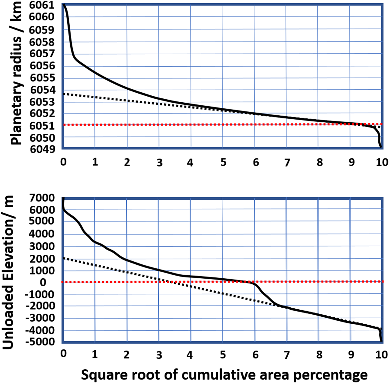
Fig. 4. Global cumulative hypsometric curves for Venus (top) and the Earth (bottom). Dashed black lines are the best linear regression fits. Modified from Rosenblatt et al. (Reference Rosenblatt, Pinet and Thouvenot1994). Dashed red lines mark nominal sea-level on Earth, while heights at Venus are referenced to a sphere of radius 6051.0 km, corresponding to the mean radius of the planet.
As significant areas of the continental surfaces are within 100 m of current sea-level, relatively small changes in terrestrial ocean depth lead to significant regressions or transgressions. However, for Venusian topography, the effects are more limited.
Marine transgression and albedo
Next, we consider another subtle influence of tectonism in determining biological evolution on planets. The early Earth was an aquaplanet, with limited sub-aerial land (e.g. Rosing et al., Reference Rosing, Bird, Sleep and Bjerrum2010; Bindeman et al., Reference Bindeman, Zakharov, Palandri, Greber, Dauphas, Retallack, Hofmann, Lackey and Bekker2018). Open ocean has an albedo of 0.06, while barren continental crust, with a granitic composition, has an albedo of 0.3 (Rosing et al., Reference Rosing, Bird, Sleep and Bjerrum2010). Plant-covered landscapes, meanwhile, have an albedo closer to 0.21 (Rosing et al., Reference Rosing, Bird, Sleep and Bjerrum2010). This implies that during periods of marine transgression, planetary albedo falls, which should, in turn, raise planetary temperatures for a given insolation and cloud cover and composition. For comparison, the Cambrian Sauk Transgression covered 60% of the currently exposed North American craton (Brasier, Reference Brasier1980).
Similarly, the extent of transgression influences the availability of other high albedo landscapes, such as desserts or ice caps. In general, such landscapes must be less common on planets where the ocean cover is more extensive. For the Earth, a rise of 100 m drowns 22.6 million km2, or 16%, of the sub-aerial surface, reducing the albedo of the affected area from approximately 0.3 for a granitic desert to 0.06 for open ocean in the affected area (Rosing et al., Reference Rosing, Bird, Sleep and Bjerrum2010). Likewise, for a vegetated landscape, the albedo is approximately 0.21 (Rosing et al., Reference Rosing, Bird, Sleep and Bjerrum2010).
Planetary albedo is estimated as follows using the proportion of the surface that has one albedo (e.g. ocean) or another.

where xA is the albedo of area A; xB is the albedo of area B and fA and fB are the relative fraction of surface with these values of albedo, respectively (shown here as percentages, but can be as a decimal fraction). As before, changes in cloud cover are ignored.
Simple scaling arguments can be used to determine the change in surface albedo, thereby, ignoring the effects of any changes to cloud cover. For illustrative purposes, a reduction in land area, associated with a 100 m sea-level rise, global albedo falls from 0.13 to 0.12.
The following expression is then used to determine the change in global temperature.

where α is the albedo, and with realistic values of emissivity, ɛ, at 0.96, Earth orbital radius, D at 1.5 × 10¹¹ m, Stefan's constant 5.67 × 10⁻⁸ watt per meter squared, per Kelvin to the fourth (W m−2 K−4). L is the current solar luminosity, 3.828 × 1026 W. The ratio of the absorbing area (A abs) versus radiating area (A rad) for the Earth may be approximated as 0.25 for its current rotation rate.
Species–area relationships
The SAR can be used to estimate the change in the number of microbial, marine or terrestrial (land) species with a change in land area (Lomolino, Reference Lomolino2000; Gray, Reference Gray2001; Azovsky, Reference Azovsky2002). This precise mathematical relationship between species richness and land-area varies with the ecosystem (Gray, Reference Gray2001; Gerstner et al., Reference Gerstner, Dormann, Vaclavık, Kreft and Seppelt2014).

which gives a linear relationship with logarithmic axes, as follows.

For shallow marine environments, C has the value of 1.7 and z has the value of 0.05 (Gray, Reference Gray2001, for illustrative purposes only).
Results
Tectonism and ocean depth
Table 4 illustrates the effect of coronae and novae on ocean depth on Venus, with assumptions regarding the area of ocean on a Venus-like planet, which lacked plate tectonics, but had Venusian-style regional tectonism. Table 4 includes the effects of ocean-ridge systems and oceanic LIPs on ocean depth from Müller et al. (Reference Müller, Sdrolias, Gaina, Steinberger and Heine2008) and Conrad (Reference Conrad2013) for comparison.
Coronae, novae and large volcanic rises are thought to be the surface manifestations of the arrival of plume heads of varying dimensions, at the base of the Venusian lithosphere (Basilevsky and Head, Reference Basilevsky and Head1998a, Reference Basilevsky and Head1998b; Krassilnikov and Head, Reference Krassilnikov and Head2003). Terrestrial rises and LIPs are, therefore, analogous (Müller et al., Reference Müller, Sdrolias, Gaina, Steinberger and Heine2008; Niu et al., Reference Niu, Shi, Li, Wu, Sun and Zhu2017). However, given the geospatial relationship of some coronae to large volcanic rises, the manner in which their plumes impinge the lithosphere is more complex than terrestrial structures. For all geospatial scenarios, the effect of novae sea-level is limited. However, the effect of both the large volcanic rises and the coronae on Venusian sea-level is comparable to that of young ocean ridges and LIPs on terrestrial sea-level. From our analysis, the volume change to oceans caused by novae would be similar to that caused by terrestrial seamounts (on the order of 100–101 m, Conrad, Reference Conrad2013).
Assuming near-constant mantle volume, swells in one area must be off-set by subsidence in others. Referring to this as compensation, Tables 5 and 6 illustrate the effect of subsidence for differing scenarios of uplift and subsidence distributions and ocean depths.
Table 5. Effect of uplift in the lowland basins and rolling plains, only, but with off-setting subsidence in the rolling plains and highlands versus the whole surface

The ocean depth has a relatively small effect as the distribution of uplift and subsidence relative to sea-level is slight.
Table 6. The effect of uplift, exclusively in the lowland basins, where off-setting subsidence is restricted to other areas of the planet; and for two depths of ocean

Using Venusian parameters, 10% of the surface is highland and not drowned with either two or three km depth of ocean; 63% is gently rolling plains of intermediate height (2–3 km above the plain) and 27% is lowland basin, <2 km above the plain (Rosenblatt et al., Reference Rosenblatt, Pinet and Thouvenot1994). Table 5 illustrates the impact of compensating subsidence for an uplift in the lowland basins and rolling uplands only, but with compensating subsidence in the highlands and rolling plains, or across the whole surface.
Next, we look at the same parameters of ocean depth and distribution of compensation, but restrict the uplift to the lowland basins. In this scenario, the change in the relative distribution of uplift to subsidence has a significant effect on sea-level change. With a shallow ocean (<2 km), the features are submerged but compensation occurs over the remaining 73.6% of the planet's surface, generating a rise in sea-level equivalent to that determined in Table 6. However, once the sea-level is increased and drowns the rolling plains, compensation by subsidence once again largely offsets rises caused by inflation of the tectonic structures.
Therefore, we conclude that the effect of regional tectonism is strongly dependent on ocean depth and where uplift is compensated. Larger areas of highland will produce proportionately greater changes in ocean depth, where uplift is dominated in the basins.
Figure 5 shows the relative impact of different Venusian volcano-tectonic structures on sea-level on hypothetical planets of varying ocean area, with the assumption that all of the features will fall into the ocean basins and there is no offsetting subsidence in these basins. Again, the depth changes are adjusted for isostatic loading.

Fig. 5. Relative change in ocean depth for various volcano-tectonic features and varying ocean area.
Overall, the effect of the larger Venusian tectonic structures on sea-level rise is within an order of magnitude of that caused by the formation of new ocean basins, with buoyant ridges, but only where the oceans are shallow and uplift is compensated by subsidence outside of the basin. Applied to the Venusian hypsometric curve, less area would be flooded than if the Earth's land distribution was used. However, as the terrestrial curve is a product of both the presence of continental crust and its erosion and deposition relative to sea-level, the difference is academic. Here, we would assume the presence of oceans will cause the continental crust to assume the broadly flat aspect in relation to the sea-level. The key factor is the volume of continental crust, which is limited in extent on Venus (perhaps 10%, Hashimoto et al., Reference Hashimoto, Roos-Serote, Sugita, Gilmore, Kamp, Carlson and Baines2008) but abundant on Earth (40% of the surface). Therefore, while a 100 m sea-level rise on Earth leads to extensive transgression, covering over 20 million km2, a similar rise on a planet with Venusian hypsometric curve will cover <10% of this area.
Importantly, while we have a good understanding of the temporal scale of tectonic processes on Earth, we do not have a similar grasp of structure formation and decay on Venus. However, future missions to Venus may clarify these temporal relationships. From here, we can then consider the rate of change of sea-level on planets that may be comparable to Venus, in terms of tectonic style.
In conclusion, while Venusian-style tectonism can produce comparable sea-level changes to those produced by plate tectonics, the hypsometric curve is critical in determining the geographical extent of the resulting transgression. For the terrestrial bimodal hypsometric curve, where there is the formation of coronae or large volcanic rises to substitute for plate tectonics, there would be significant transgressions covering land areas comparable to those seen in the Phanerozoic. Therefore, the Venusian mode of tectonism could drive the biological diversification and mass extinction seen on Earth (Brasier, Reference Brasier1980, Reference Brasier1982; Banerjee et al., Reference Banerjee, Schidlowski, Siebert and Brasier1997; Banerjee and Mazumdar, Reference Banerjee and Mazumdar1999; Squire et al., Reference Squire, Campbell, Allen and Wilson2006; Peters and Gaines, Reference Peters and Gaines2012; Landing and Kouchinsky, Reference Landing and Kouchinsky2016; Clemmensen et al., Reference Clemmensen, Glad, Gunver and Pedersen2017; Karlstrom et al., Reference Karlstrom, Hagadorn, Gehrels, Matthews, Schmitz, Madronich, Mulder, Pecha, Giesler and Crossey2018; Latif et al., Reference Latif, Xiao, Riaz, Wang, Khan, Hussein and Khan2018; Wei et al., Reference Wei, Planavsky, Tarhan, Chen, Wei, Li and Ling2018; Paterson et al., Reference Paterson, Edgecombe and Lee2019). However, while this is true, the Venusian mode of regional tectonism is not associated with a comparable hypsometric curve. Therefore, the transgressive effect would be more limited if the planet lacked similarly extensive areas of continental crust as the Earth.
Marine transgressions and planetary albedo
Next, we consider whether a realistic marine transgression will change the albedo sufficiently to alter the overall temperature of the planet. We take the Earth's hypsometric curve and land area, then raise sea-level by 100 m. The early Earth was an aquaplanet, with limited sub-aerial land (Flament et al., Reference Flament, Coltice and Rey2008; Rosing et al., Reference Rosing, Bird, Sleep and Bjerrum2010; Bindeman, et al., Reference Bindeman, Zakharov, Palandri, Greber, Dauphas, Retallack, Hofmann, Lackey and Bekker2018). The albedo of open ocean is considerably lower than that of continental crust (0.06 versus 0.30). Applying a transgression of 100 m to the Earth's current hypsometric curve will result in an inundation of 22 million km2 of land (14.7% of the total land area). From simple surface area relationships, and ignoring any changes in cloud cover, planetary albedo is reduced from 0.13 to 0.12 during the accompanying transgression on vegetation-free land.
Likewise, for a planet with a terrestrial land area of 149 million km2, terrestrial hypsometric curve and plant-coverage, a 100 m sea-level rise reduces the land area to 127.5 million km2. The corresponding albedo is 0.0975. For the equivalent vegetated planet, but without the transgression, the albedo will be 0.1035. Ignoring variation in cloud-cover, the difference in albedo is 0.006, which changes the effective surface temperature by 0.28 K. Table 7 summarizes these results for surface albedo and temperature.
Table 7. Changes in surface albedo and corresponding temperature for three scenarios relative to a planet with terrestrial land area (149 million km2 and ocean area 361.9 million km2) and no vegetation

The effect of cloud-cover is ignored.
Therefore, we conclude that a 100 m sea-level rise and accompanying transgression on the terrestrial hypsometric curve has a small but measurable effect on global temperature. The effect of transgressions is greatest for planets with greater areas of more reflective non-vegetated land.
Table 8 shows the area of land drowned during terrestrial Phanerozoic transgressions, for comparison. The Cambrian (Sauk) transgressions were more extensive than would be expected today because the hypsometric curve was different. The Cambrian terrain was much closer to sea-level, probably as a result of late Proterozoic glaciation (Keller et al., Reference Keller, Husson, Mitchell, Bottke, Gernon, Boehnke, Bell, Swanson-Hysell and Peters2019). Therefore, sea-level rises, on the order of 90 m inundated far larger areas of the continent than would be seen today.
Table 8. Changes in surface albedo for the six Phanerozoic transgressions

For the Cambrian (Sauk) transgressions, the value for land albedo is that of barren granitic desert (0.3), while for later transgressions, surface albedo is set at 0.21 for vegetated landscape. Ocean albedo is set at 0.06. Comparison is made for contemporaneous land area (29%).* The value for the Sauk transgression is based on a change in area from granitic desert to ocean; while the latter ones are from vegetated landscapes to ocean.
Table 9 illustrates the potential change in surface temperature for a given albedo and ignoring the effects of cloud cover.
Table 9. Changes to surface temperature for a given surface albedo and ignoring the effects of clouds

In this analysis, transgressions consistently drive rises approximating 0.3 K, relative to current land area (149 million km2) with vegetated or *non-vegetated landscapes and land albedo values equivalent to those in Table 6.
We show that terrestrial transgressions will alter surface temperature, by altering surface albedo, in the absence of changes to cloud cover. Therefore, aside from altering the distribution of habitats, transgressions can also alter the surface temperature. The mode of tectonism, therefore, has evolutionary impacts that extend beyond altering, eliminating or creating habitats.
Marine transgressions and evolutionary diversification
In this section, we review the likely impacts of sea-level change on biodiversity and evolution. We consider, first, the impact of plate tectonics, then Venusian tectonics. Clearly, we cannot anticipate the path that the evolution of life will take on an alien world, other than to specify, by definition, evolution is an increase in the complexity of all life. Now, specifically, this increase in complexity is manifest as an increase in the complexity of the information present, following the rules of information entropy. We can illustrate the increase, or change, in complexity through the SAR (Lomolino, Reference Lomolino2000; Gray, Reference Gray2001; Azovsky, Reference Azovsky2002; Neigel, Reference Neigel2003).
If we apply terrestrial marine values of C as 1.7 and z as 0.05, then for every increase of one million km2, the number of marine species would increase by 52. While SARs are unique to each class of organism in each environment, the principle applies to all terrestrial life, whether microbial or multicellular (Lomolino, Reference Lomolino2000). Therefore, one expects that marine transgression or regression must, by definition, increase or decrease species diversity. Initial flooding would be expected to eliminate subaerial habitats, while creating novel shallow marine habitats, and vice versa.
The precise impact of regression or regression depends on the hypsometric curve for the planet in question. Planets with strongly bimodal distributions, where much of the land lies close to sea-level, should expect strong changes in species diversity with changes in sea-level. Planets with steeper hypsometric curves will show proportionately lower changes in species diversity as transgression or regression will be more limited in extent.
Discussion
In this paper, we discuss the impact of Venusian-style tectonism on ocean depth, given various scenarios for ocean area. We then consider the knock-on effects of ocean transgression on any biosphere. In particular, we ask how marine transgressions might affect the availability of habitats, nutrients and, finally, climate.
While we have used relatively simple models to determine the volume of each structure, volume calculations for the large volcanic rises come close to the values determined by other means, thereby validating the overall approach (King and Adam, Reference King and Adam2014; Hoggard et al., Reference Hoggard, Parnell-Turnerc and Whited2020). We can conclude that planets with Venusian-style regional tectonism can experience comparable transgression events to those associated with terrestrial tectonism, whether this is hot spot-related or plate-tectonics. However, the magnitude of sea-level rise is dependent on the location of the event(s) that give rise to it and the location of any associated subsidence. Applied to our model planet, Venus, with its distribution of highland, upland and lowland crust, then only in the extreme scenario, where we have relatively shallow seas and uplift confined to the basins, do we see large transgressions comparable in magnitude to those seen on Earth. In most other scenarios that we tested, sea-level changes are far more modest, on the order of a few metres or less. However, we note that even the modest scale of the rises that are seen in these models would still have a notable impact on coastal erosion and sea-level advance. The relationship between sea-level rise and erosion (Bruun equation 1) would cause a retreat two orders of magnitude greater than the observed rise, potentially releasing considerable additional debris and nutrients to any coastal environment (Zhang, Reference Zhang1998; Zhang et al., Reference Zhang, Douglas and Leatherman2004).
The precise magnitude of any transgression is also dependent on the planet's hypsometric curve. For the Earth, tens of millions of square kilometres of land lie within 200 m of current sea-level. Modest rises, therefore, bring about significant changes to the location of coastlines. On Venus, which lacks oceans, the hypsometric curve appears to principally relate to the location of volcano-tectonic structures, rather than to sedimentation or the presence of widespread sialic crust (Hashimoto et al., Reference Hashimoto, Roos-Serote, Sugita, Gilmore, Kamp, Carlson and Baines2008). Other worlds could be envisaged that have a greater prevalence of sialic crust but regional tectonism – as appears the case in the terrestrial Archean era (Rozel et al., Reference Rozel, Golabek, Jain, Tackley and Gerya2017). Such worlds may have hypsometric curves that are a closer match to the current Earth than barren Venus.
Next, we examined the effect of transgression on planetary albedo, using the terrestrial transgressions as examples. As one might expect from changing the land-sea distribution, transgression lowers global albedo and, therefore, can raise planetary temperature; precisely the mechanism identified by Rosing et al. (Reference Rosing, Bird, Sleep and Bjerrum2010) to keep the early Earth warm. In this instance, we are looking at more modest changes in sea-level and more modest changes in temperature; however, the effect may still yield biological changes. Moreover, changes to temperature would be expected to generate further change through positive and negative feedback mechanisms. For example, increases in temperature increase the rate of respiration of any extant microorganisms (Heimann and Reichstein, Reference Heimann and Reichstein2008). Increases in respiration lead to amplification in carbon dioxide production and hence, further rises in the proportion of greenhouse gases. For example, Scheffer et al. (Reference Scheffer, Brovkin and Cox2006) suggest that feedback will promote a 15–78% increase in temperature on century timescales. Secondly, loss of land surface and rises in temperature will reduce any ice cover (Pistone et al., Reference Pistone, Eisenman and Ramanathan2019). This process will also lead to a reduction in albedo and further rises in temperature. A final and critical feedback concerns the well-known carbonate-silicate cycle (Walker et al., Reference Walker, Hays and Kasting1981). Increases in the erosion of silicate bedrock increase carbon sequestration on millennial and longer timescales. The rate of this process increases with higher temperature. Therefore, when considering the impact of lower albedo on planetary temperature, one must also consider how increases in the rate of erosion of non-transgressed land will affect the longer-term changes in the temperature of the planet.
Marine photosynthetic organisms are known to affect cloud formation (Rosing et al., Reference Rosing, Bird, Sleep and Bjerrum2010). Enhanced erosion at the wave-cut margins (razoring), which is associated with transgression, should lead to blooms of microorganisms in the oceans, as marine transgression liberates nutrients. On Earth, plants and algae produce the majority of cloud-condensation-nuclei (CCNs, Rosing et al., Reference Rosing, Bird, Sleep and Bjerrum2010). Blooms of algae might be expected consequent to marine transgression, as ocean waters erode material from the receding continental margins and liberate nutrients. Conversely, there is a significant contribution to CCN from feldspar particles, which initiate the formation of ice crystals (Kiselev et al., Reference Kiselev, Bachmann, Pedevilla, Cox, Michaelides, Gerthsen and Leisner2017). Reduction in the availability of land would reduce the abundance of feldspar aerosols, thereby reducing cloud formation, particularly on planets with limited biospheres. The uncertainty in the confounding effects of wind versus wave-driven erosion on the availability of different CCN means that we did not pursue cloud-driven albedo changes in this work but seems a fertile area for further work.
Similarly, while the Earth likely, currently, experiences a net regassing of the mantle (Korenaga et al., Reference Korenaga, Planavsky and Evans David2017), planets lacking plate tectonics will progressively degas at a rate dependent on their mass, internal radiogenic budget and the mode of mantle convection (Schaefer and Sasselov, Reference Schaefer and Sasselov2015). Without a means to lose surface water, either to space or by tectonism to the mantle, ocean levels will increase, in a declining upward trend, leading to progressive drowning of surface features.
What are the likely impacts on the evolution of life on planets that experience Venus-like tectonism? If we ignore the risk of complete drowning of the surface through progressive degassing or sedimentation, variations in tectonic rate will lead to transgressions and regressions in a manner similar to those seen on Earth but of lower magnitude. To quantify some of the likely effects, we use SAR as a proxy for species distribution with land (or shallow marine) areas. Focussing on transgression and values for marine species taken from Gray (Reference Gray2001), we can readily show that increases in shallow marine environments will also increase species richness (the variety of species present). We also note that allopatric speciation (the formation of new species following geographical separation) is facilitated by the formation of new landscapes (Heenan and McGlone, Reference Heenan and McGlone2013; Rahbek et al., Reference Rahbek, Borregaard, Colwell, Dalsgaard, Holt, Morueta-Holme, Nogues-Bravo, Whittaker and Fjeldså2019). During marine transgression, land habitats are eliminated and marine habitats are created. For planets with predominantly marine biotas, such as the terrestrial Cambrian and Ordovician eras, the creation of an abundance of habitats is associated with strong evolutionary diversification. The loss of many of these habitats in the late Ordovician is associated with mass extinction (Barash, Reference Barash2014).
Therefore, if marine transgression was a trigger (or one of a few triggers) for the Cambrian Explosion (Peters and Gaines, Reference Peters and Gaines2012) and for various extinction events (Solé et al., Reference Solé, Fernández and Kauffman2003; Squire et al., Reference Squire, Campbell, Allen and Wilson2006; Bond and Wignall, Reference Bond and Wignall2008; Vodráqková et al., Reference Vodráqková, Frýda, Suttner, Koptíková and Tonarová2013; Barash, Reference Barash2014; Brocke et al., Reference Brocke, Fatka, Lindemann, Schindler and Ver Straeten2015; López-Villalta, Reference López-Villalta2016; Percival et al., Reference Percival, Davies, Schaltegger, De Vleeschouwer, Da Silva and Föllmi2018), then we can anticipate Venusian-style regional tectonism can drive similar evolutionary processes on worlds that experience these kinds of tectonic events. The magnitude of the transgression depends on the location of any uplift and associated subsidence; but also, on the depth of any oceans.
That planets that lack plate tectonics may progressively drown must also be considered. Degassing could be prompt, so that the majority of available water is released early, with little variation later on. To such worlds, volcano-tectonic activity might then build subaerial structures, if water depths are not extreme. Schaefer and Sasselov (Reference Schaefer and Sasselov2015) consider different planetary models with different rates of degassing. The largest worlds in their models may take a few billion years to degas, while others show prompt degassing. Regassing was relatively fast for some of their model worlds – however, these models were assumed to have plate tectonics. Rapid growth of continental crust, which may choke off plate tectonics, is rarely considered (Lenardic et al., Reference Lenardic, Moresi, Jellinekc and Manga2005). Determining whether planets will host plate tectonics for realistic masses and rates of continental growth awaits further modelling. Planets that initially have hot stagnant lids may have regional tectonism, like Venus, but grow continental crust so quickly that the surface becomes too buoyant for subduction to occur (Kite et al., Reference Kite, Manga and Gaidos2009).
Ultimately, the impact of changes to ocean depth on evolutionary progression will clearly be context-related. If one considers the Earth, then on a planet that was otherwise rather barren in the Neoproterozoic, marine transgression may have eliminated (or created) prokaryotic niches, but little else until late in the era. More fundamentally, 3.0–2.7 billion years ago, most of the Earth's continental crust was submerged (Flament et al., Reference Flament, Coltice and Rey2008; Bindeman et al., Reference Bindeman, Zakharov, Palandri, Greber, Dauphas, Retallack, Hofmann, Lackey and Bekker2018; Cawood et al., Reference Cawood, Hawkesworth, Pisarevsky, Dhuime, Capitanio and Nebel2018) but the advent of modern plate tectonics brought about (or as it is least associated with) the emergence of 90% of the current land surface. Shortly, thereafter there is a succession of glaciations, which one would expect following an increase in global albedo that would be associated with the emergence of land (a change in albedo from 0.06 to 0.3, Rosing et al., Reference Rosing, Bird, Sleep and Bjerrum2010). Moreover, during the period from 2.7 to 2.5 Gya, most of the large continental bodies are thought to have been assembled in the Kenorland supercontinent (Yakubchuk, Reference Yakubchuk2019). The formation of the supercontinent would be associated with uplift and enhanced weathering, and a decrease in sea-level. The subsequent dispersion of Kenorland after 2.5 Gy would be accompanied by marine transgression as new, buoyant oceanic lithosphere raised the level of the ocean floor. It is noteworthy, then that the GOE occurs in the time-frame associated with marine transgression and the formation of new, shallow, ocean margins (Philippot et al., Reference Philippot, Ávila, Killingsworth, Killingsworth, Tessalina, Baton, Caquineau, Muller, Pecoits, Cartigny, Lalonde, Ireland, Thomazo, van Kranendonk and Busigny2018).
In the Cambrian and early Ordovician, transgressions are associated with great biological diversification. Conversely, during the Devonian, transgressions are linked to global and regional extinction events. In turn, extinction events lead to the opening of new niches for life, promoting innovation in the longer term. Likewise, the biological innovations of the Cambrian that led to us follow the wholesale extinction of the Ediacaran lineages. Transgressions may thus be as much a razor for life as they are for the bedrock, over which they sweep.
In this regard, Rosing et al. (Reference Rosing, Bird, Sleep and Bjerrum2010) identify a final factor of relevance to the long-term survival of life on a planet. Consider a world lying near the inner edge of the habitable zone, where global plate tectonics does not operate. Here, degassing continues and the surface progressively drowns. While there are immediate losses of biological niche spaces on land (and the growth of marine niche spaces), there will be a decrease in planetary albedo that is associated with the loss of continental surface. Therefore, in the longer term, progressive transgression could warm the planet through the reduction in albedo, so that it experiences a thermal runaway. Additional feedbacks clearly need consideration.
There are a considerable number of variables that can influence ocean depth on planets where regional tectonic processes dominate. As a first step, this paper examines a few of these variables, using Venusian tectonism as a model starting point. However, we hope that it is clear that there are several other factors that should be considered if we are then to extrapolate to any impact of tectonic style on habitability and the evolvable potential of any life that emerges.
Acknowledgements
I would like to thank Norm Sleep for helpful discussions on an earlier draft of the manuscript; and the anonymous reviewer whose salient comments have both broadened and enhanced this manuscript. I would also like to express some a final thank you for some final editorial comments which have further broadened the work.


