Stellar parameters

Regarding our study, stellar parameters are of pivotal importance for the calculation of stellar HZs as well as for orbital stability simulations of possible exomoons and Trojan objects. Most relevant parameters of the Kepler-16(AB) system have been previously reported by Doyle et al. (Reference Doyle, Carter, Fabrycky, Slawson, Howell, Winn, Orosz, Prša, Welsh, Quinn, Latham, Torres, Buchhave, Marcy, Fortney, Shporer, Ford, Lissauer, Ragozzine, Rucker, Batalha, Jenkins, Borucki, Koch, Middour, Hall, McCauliff, Fanelli, Quintana, Holman, Caldwell, Still, Stefanik, Brown, Esquerdo, Tang, Furesz, Geary, Berlind, Calkins, Short, Steffen, Sasselov, Dunham, Cochran, Boss, Haas, Buzasi and Fischer2011), as they announce a transiting circumbinary planet observed by the Kepler spacecraft. Kepler-16A was identified as a K-type main-sequence star with effective temperature, radius and mass given as (see Table 1) 4450 ± 150 K, 0.6489 ± 0.0013 R _⊙ and 0.6897 ± 0.0035 M _⊙, respectively. Here the relative uncertainty bar is the largest for the stellar effective temperature (see Table 2).

Table 2. Percentage uncertainty of Kepler-16 parameters

However, less information has been conveyed for Kepler-16B, which based on its mass of about 0.20255 M _⊙ (Doyle et al., Reference Doyle, Carter, Fabrycky, Slawson, Howell, Winn, Orosz, Prša, Welsh, Quinn, Latham, Torres, Buchhave, Marcy, Fortney, Shporer, Ford, Lissauer, Ragozzine, Rucker, Batalha, Jenkins, Borucki, Koch, Middour, Hall, McCauliff, Fanelli, Quintana, Holman, Caldwell, Still, Stefanik, Brown, Esquerdo, Tang, Furesz, Geary, Berlind, Calkins, Short, Steffen, Sasselov, Dunham, Cochran, Boss, Haas, Buzasi and Fischer2011) is identified as a red dwarf. But Kepler-16B's effective temperature needs to be determined as well to compute the HZ for the Kepler-16 binary system. Thus, to determine Kepler-16B's stellar effective temperature, we utilize the mass – effective temperature relationship by Mann et al. (Reference Mann, Gaidos and Ansdell2013). They have analysed moderate resolution spectra for a set of nearby K and M dwarfs with well-known parallaxes and interferometrically determined radii to define their effective temperatures, among other quantities. They have also adopted state-of-the-art PHOENIX atmosphere models, as described. Thus, we conclude that the effective temperature of Kepler-16B is 3308 ± 110 K (see Fig. 1). Here the uncertainty bar has been estimated based on the results of similar objects included in the sample. From other work as, e.g. by Kirkpatrick et al. (Reference Kirkpatrick, Henry and McCarthy1991) and Baraffe et al. (Reference Baraffe, Chabrier, Allard and Hauschildt1998) the spectral type of Kepler-16B has been deduced as ~M3 V. Both the effective temperature and radius of Kepler-16B are important for determining the different types of HZs of the Kepler-16(AB) system (see the section ‘Stability investigations for Earth-mass exomoons and Trojans’).

Fig. 1. Depiction of the effective temperature of Kepler-16B determined via an empirical formula given by Mann et al. (Reference Mann, Gaidos and Ansdell2013) that relates the mass to the effective temperature, and vice versa, for M dwarf stars. By knowing the mass of Kepler-16B, its effective temperature can be extracted, resulting in an effective temperature of 3308 ± 110 K. In addition, a subset of the sample of M dwarf stars is depicted, used to derive the adopted empirical formula.

The Kepler-16 HZ

A crucial aspect of this study is the evaluation of Kepler-16's HZ. The HZ is a region around a star or a system of stars in which terrestrial planets could potentially have surface temperatures at which liquid water could exist, given a sufficiently dense atmosphere (e.g., Kasting et al., Reference Kasting, Whitmore and Reynolds1993; Jones et al., Reference Jones, Sleep and Chambers2001; Underwood et al., Reference Underwood, Jones and Sleep2003). When determining the HZ, both inner limits and outer limits are calculated, in response to different types of criteria, thus defining the HZ. The determination of the location of the HZ is significant in the context of theoretical studies as well as for the purpose of planet search missions (e.g., Lammer et al., Reference Lammer, Bredehöft, Coustenis, Coustenis, Khodachenko, Kaltenegger, Grasset, Prieur, Raulin, Ehrenfreund, Yamauchi, Wahlund, Grießmeier, Stangl, Cockell, Kulikov, Grenfell and Rauer2009; Kasting et al., Reference Kasting, Kopparapu, Ramirez and Harman2014; Kaltenegger, Reference Kaltenegger2017, and references therein).

Inner limits previously used for stellar HZs include those set by the recent Venus (RV), the runaway greenhouse effect and the onset of water loss. Furthermore, the outer limit of the stellar HZ has been set by the first CO₂ condensation, the maximum greenhouse effect for a cloud-free CO₂ atmosphere and the early Mars (EM) setting. For example, Kasting et al. (Reference Kasting, Whitmore and Reynolds1993) describe the runaway greenhouse effect such that the greenhouse phenomenon is enhanced by water vapour, thus promoting surface warming. The latter further increases the atmospheric vapour content, thus resulting in an additional rise of the planet's surface temperature. Consequently, this will lead to the rapid evaporation of all surface water. On the other hand (see, e.g., Underwood et al., Reference Underwood, Jones and Sleep2003), the water loss criterion means that an atmosphere is warm enough to have a wet stratosphere, from where water is gradually lost by atmospheric chemical processes to space.

Table 3 shows the HZ limits for Kepler-16A, treated as a single star, for tutorial reasons. Here GHZ denotes the general HZ, bracketed by the runaway greenhouse and maximum greenhouse criteria, whereas RVEM denotes the kind of HZ, defined by the settings of RV and early Mars; this latter type of HZ is also sometimes referred to as (most) optimistic HZ; see, e.g., Kaltenegger (Reference Kaltenegger2017) and references therein. Figure 2 and Tables 3 and 4 convey the results for the various HZ limits as well as for the GHZ and RVEM. The most recent results based on Kopparapu et al. (Reference Kopparapu, Ramirez, Kasting, Eymet, Robinson, Mahadevan, Terrien, Domagal-Goldman, Meadows and Deshpande2013, Reference Kopparapu, Ramirez, SchottelKotte, Kasting, Domagal-Goldman and Eymet2014) have been included as well, which indicate updated HZ limits. For the inner and outer HZ limits, they assumed H₂O and CO₂ dominated atmospheres, respectively, while scaling the background N₂ atmospheric pressure with the radius of the planet. Moreover, from the said climate model, several equations were generated, which correspond to select inner and outer HZ limit criteria.

Fig. 2. Inner and outer HZ limits for Kepler-16A (single star approach) while comparing two different determination methods. We also include information on the inherent statistical uncertainties of those based on Press et al. (Reference Press, Flannery, Teukolsky and Vetterling1986) (see also Table 3). The blue data correspond to the inner and outer HZ boundaries as expected from utilizing the method of Kasting et al. (Reference Kasting, Whitmore and Reynolds1993) with updates by Underwood et al. (Reference Underwood, Jones and Sleep2003) and Selsis et al. (Reference Selsis, Kasting, Levrard, Paillet, Ribas and Delfosse2007). Conversely, the red data correspond to the inner and outer HZ limits as expected from utilizing the method specified by Kopparapu et al. (Reference Kopparapu, Ramirez, Kasting, Eymet, Robinson, Mahadevan, Terrien, Domagal-Goldman, Meadows and Deshpande2013, Reference Kopparapu, Ramirez, SchottelKotte, Kasting, Domagal-Goldman and Eymet2014).

Table 3. Single star habitable zone limits

Note: Kas93: Kasting et al. (Reference Kasting, Whitmore and Reynolds1993), Und03: Underwood et al. (Reference Underwood, Jones and Sleep2003), Kop1314: Kopparapu et al. (Reference Kopparapu, Ramirez, Kasting, Eymet, Robinson, Mahadevan, Terrien, Domagal-Goldman, Meadows and Deshpande2013, Reference Kopparapu, Ramirez, SchottelKotte, Kasting, Domagal-Goldman and Eymet2014).

Table 4. Statistical uncertainties

Note: For references, see comments of Table 3. Min-Max means that the minimum/maximum values for the luminosities and effective temperatures are applied. Statis means adequately applied statistical uncertainty propagation.

Surely, most of our study focuses on Kepler-16 as a binary thus taking into account both Kepler-16A (an orange dwarf) and Kepler-16B (a red dwarf); see Table 1 for data. The computation of the GHZ and RVEM of Kepler-16(AB) follows the work by Cuntz (Reference Cuntz2014, Reference Cuntz2015) and Wang & Cuntz (Reference Wang and Cuntz2017). Information is given in Fig. 3; here RHZ refers to the so-called radiative habitable zone (applicable to both the GHZ and RVEM), which is based on the planetary climate enforcements set by both stellar components, while deliberately ignoring the orbital stability criterion regarding a possible system planet. Figure 3 indicates the inner and outer RHZ limits with the inner HZ limit defined as the maximum radial distance of the inner RHZ (red lines) and the outer HZ limit defined as the minimum radial distance of the outer RHZ (blue lines). This approach conveys the HZ region for GHZ (darkest green) and RVEM (medium green) criteria (see also Table 5). As expected, the RVEM criteria produce a more generous HZ region. We also indicate the orbital stability limit (black dashed line) based on Holman & Wiegert (Reference Holman and Wiegert1999), referred to as ɑ _orb. In fact, it is found that the widths of the GHZ and RVEM for Kepler-16(AB) are significantly less than for Kepler-16A (single-star approach), owing to the additional criterion of orbital stability for possible system planets.

Fig. 3. Depiction of the RHZ for the GHZ and RVEM criteria based on methods given by Cuntz (Reference Cuntz2014, Reference Cuntz2015) and Wang & Cuntz (Reference Wang and Cuntz2017). In both plots the red and blue lines correspond to the inner and outer RHZ limits with the inner HZ limit defined as the maximum radial distance of the inner RHZ (red lines) and the outer HZ limit defined as the minimum radial distance of the outer RHZ (blue lines). This approach produces the conventional HZ region for GHZ (darkest green) and RVEM (medium green) criteria. As expected the RVEM criteria produce a more generous HZ region as shown. Lastly, the black dashed line represents the orbital stability limit, calculated using the formula provided by Holman & Wiegert (Reference Holman and Wiegert1999) for P-type orbits, in which bodies exterior to that line are orbitally stable while bodies interior to that line are orbitally unstable.

Table 5. GHZ and RVEM RHZs of binary system

Note: The RHZ bounds have previously been referred to as RHLs (Cuntz, Reference Cuntz2014). Here the innermost and outermost points of these limits are reported, which are of different relevance for setting the respective RHZ.

Previous work by Mischna et al. (Reference Mischna, Kasting, Pavlov and Freedman2000) argues that the HZ about a main-sequence star might be further extended if CO₂ cloud coverage is assumed. In the case of the Sun, this assumption would amount to an outer limit of 2.40 AU for the hereupon defined extended habitable zone (EHZ)Footnote ¹. Von Bloh et al. (Reference von Bloh, Bounama, Cuntz and Franck2007) have explored the habitability around Gliese 581 with focus on the possible planet GJ 581d. They argue that the RHZ could be further extended if the atmospheric structure is determined by particularly high-base pressures. Thus, the outer limit for the EHZ is not very well constrained, but could be parameterized as $\epsilon \sqrt {L}$ with ε in the likely range between 2.0 and 3.0 and L defined as stellar luminosity (in units of solar luminosity). Hence, ε = 2.4 corresponds to the value of Mischna et al. (Reference Mischna, Kasting, Pavlov and Freedman2000). Results for the EHZ of Kepler-16(AB) are given in Fig. 4 and Table 6.

Fig. 4. Different outer boundaries (blue lines) of the EHZ resulting from the different epsilon values ranging from ε = 2.0 (innermost blue line) to ε = 3.0 (outermost blue line). A median value of ε = 2.5 has been chosen for our definition of the EHZ akin to Mischna et al. (Reference Mischna, Kasting, Pavlov and Freedman2000), which is also adopted for our analysis in the subsequent Figs. 7, 8 and 10 and depicted as the lightest green regions.

Table 6. EHZ of Kepler-16(AB)

Another aspect of study is that concerning the GHZ and RVEM, we also have explored the impact of the observational uncertainties of the stellar luminosities on inner and outer limits of the RHZs (see Figs. 5 and 6). It is found that the uncertainty in the stellar luminosity ΔL moves the inner and outer limits of both the GHZ and the RVEM by about ±6%. Our results are summarized in Table 7. Here we also see that the inner limits of both the GHZ and RVEM are set by the additional criterion of orbital stability regarding possible circumbinary planets referred to by Cuntz (Reference Cuntz2014) as PT habitability. Additionally, it is found that the HZ around Kepler-16A (if treated as a single star) would be significantly more extended than the HZ of Kepler-16(AB). Thus, Kepler-16B notably reduces the prospect of habitability in that system.

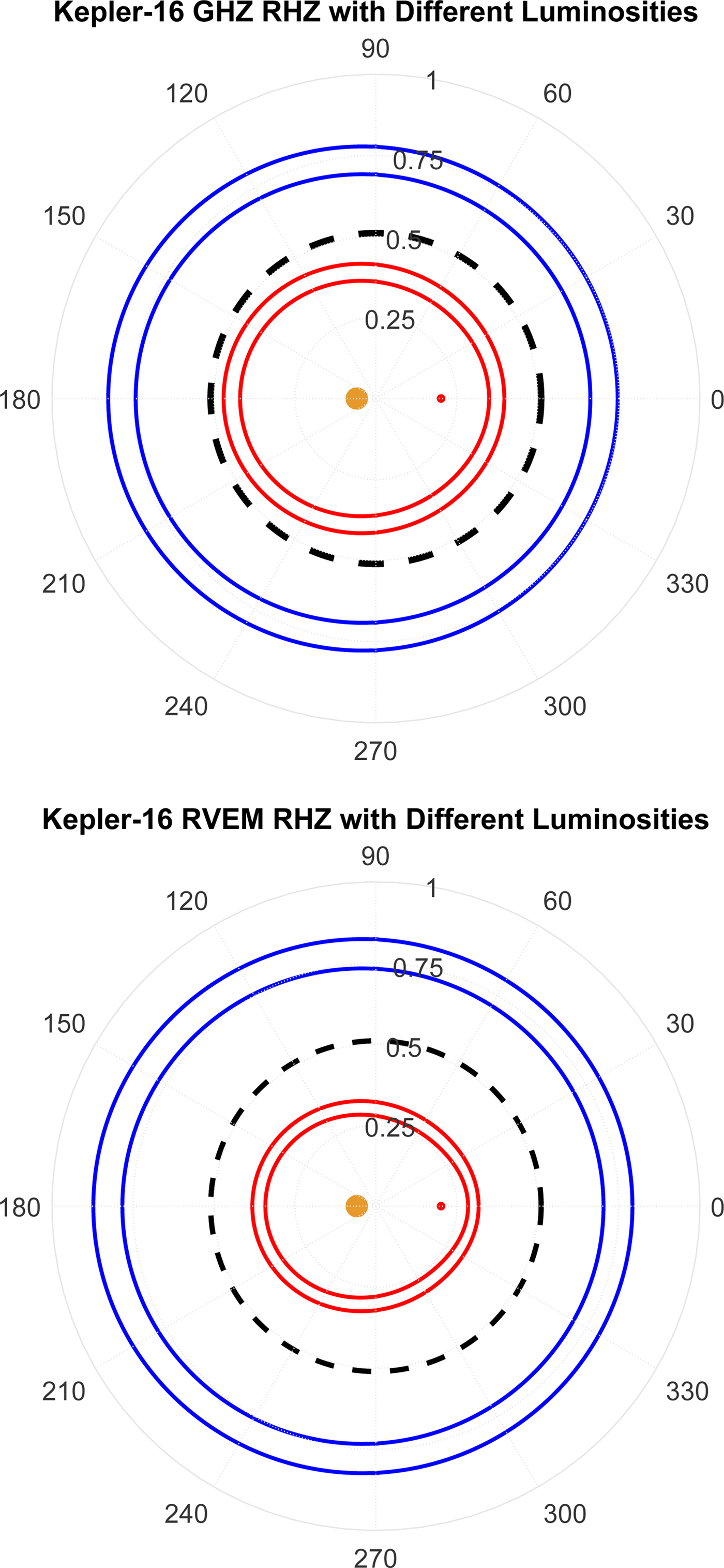
Fig. 5. Depiction of the inner and outer boundaries of the GHZ and RVEM, while utilizing the upper and lower bounds of the stellar luminosities to illustrate how the uncertainty in the luminosity affects the determination of the HZs. In both plots the inner and outer HZ limits are shown in red and blue, respectively, with the inner sets of red and blue lines corresponding to the lower bound luminosity and the outer sets of red and blue lines corresponding to the upper bound luminosity. As expected, the upper bound luminosity shifts the GHZ and RVEM limits outward while the lower bound luminosity shifts those limits inward.

Fig. 6. Similar to Fig. 5, as this figure combines the inner and outer boundaries for the GHZ and RVEM criteria while also incorporating the upper and lower luminosity bounds; its emphasis is to illustrate the extents of the achievable HZs based on luminosity and HZ criteria specification. Additionally, the black dashed line represents the orbital stability limit. The blue and red dotted lines correspond to the minimum possible inner limits (associated with the lower bound luminosity) for the GHZ and RVEM, respectively. The blue and red solid lines correspond to the maximum possible outer limits (associated with the upper bound luminosity) for GHZ and RVEM, respectively.

Table 7. Comparison of habitable zone limits

Note: (L ⁺) and (L ⁻) indicate L ± ΔL, respectively, with variations in T _eff and R simultaneously applied to both stellar components (see Table 1). ΔHZ indicates the width of the HZ with consideration of the orbital stability limit, if applicable. PT conveys that the P-type HZ is truncated due to the additional requirement of orbital stability.

Stability investigations for Earth-mass exomoons and trojans

Previously, QMC12 have exemplary case studies for the orbital stability of Earth-mass objects (i.e., Trojan exoplanet or exomoon) in the Kepler-16(AB) system. Their numerical methods were based on the Wisdom-Holman mapping technique and the Gragg-Burlisch-Stoer algorithm (Grazier et al., Reference Grazier, Newman, Varadi, Goldstein and Kaula1996). The resulting equations of motion were integrated forward in time for 1 million years using a fixed/initial (WH/GBS) time step. QMC12 showed that, in principle, both Trojan exoplanets and exomoons are able to exist in the Kepler-16(AB) system. Figures 7 and 8 show the results by QMC12 together with the updated system's HZs, i.e., the GHZ, RVEM and EHZ. It is found that the orbital settings of those objects are within the EHZ (with ε ≲ 2.2) or within the RVEM if upper limits of the stellar luminosities, consistent with the observational uncertainties, are considered.

Fig. 7. Illustration of previous results by QMC12 with updated HZ regions. (a) Depiction of an S-type captured Earth-mass exomoon (black in QMC12); the primary and secondary stars (orange and red in QMC12, respectively) and the Saturnian planet Kepler-16b are also given (magenta in QMC12). (b) Depiction of a possible Trojan exomoon in a rotating reference frame (black in QMC12). The darkest green region represents the GHZ, the medium green region represents the RVEM, and the lightest green region represents the EHZ. The dashed yellow line represents the outer limit of the GHZ if the stellar luminosities are assumed at their upper limits as informed by the observational uncertainties.

Fig. 8. Illustration of the previous results by QMC12 with updated HZ regions. (a) Depiction of a stable S-type coformed Earth-mass exomoon (black in QMC12); the primary and secondary stars (orange and red in QMC12, respectively) and the Saturnian planet Kepler-16b are also given (magenta in QMC12). (b) Depiction of an unstable S-type coformed Earth-mass exomoon (black in QMC12). See Fig. 7 for information on the colour coding of the HZs.

In order to better understand the dynamical domain of possible exo-Trojans, we perform additional 5000 stability simulations using a modified version of the mercury6 integration package that is optimized for circumbinary systems (Chambers et al., Reference Chambers, Quintana, Duncan and Lissauer2002). In these simulations, we adopt the orbital parameters from Doyle et al. (Reference Doyle, Carter, Fabrycky, Slawson, Howell, Winn, Orosz, Prša, Welsh, Quinn, Latham, Torres, Buchhave, Marcy, Fortney, Shporer, Ford, Lissauer, Ragozzine, Rucker, Batalha, Jenkins, Borucki, Koch, Middour, Hall, McCauliff, Fanelli, Quintana, Holman, Caldwell, Still, Stefanik, Brown, Esquerdo, Tang, Furesz, Geary, Berlind, Calkins, Short, Steffen, Sasselov, Dunham, Cochran, Boss, Haas, Buzasi and Fischer2011) for the binary components and the Saturnian planet. We also consider Earth-mass objects with different initial conditions. Table 8 conveys the initial conditions for exomoon sample cases, which are: the semimajor axis a, eccentricity e, inclination i, argument of periastron ω and mean anomaly M for each body. A simulation is terminated when the Earth-mass body either crosses the binary orbit or has a radial distance from the centre of mass greater than 100 AU; this will be viewed as an ejection.

Table 8. Initial conditions for exomoon sample cases

Note: Initial conditions in terms of orbital elements for the binary (Kepler-16(AB)), the Saturnian planet (Kepler-16b) and the possible Earth-mass exomoon. These orbital elements can be used to reproduce our new results (Fig. 11) and the previous results of QMC12 (Figs. 7 and 8).

The orbital evolution of the four bodies is evaluated on a 10 Myr timescale. The initial orbital elements are chosen using uniform distributions. The initial semimajor axis of the Earth-mass object is selected from values ranging from 0.6875 AU to 0.7221 AU (i.e., ± 0.5 Hill radii); furthermore, eccentricities are limited to 0.1 and inclinations are limited to 1°. The initial argument of periastron and mean anomalies are selected randomly between 0° and 360°. The statistical distributions of the surviving population are shown in Fig. 9 to illustrate possible correlations between parameters.

Fig. 9. Distributions of the initial semimajor axis a, eccentricity e, inclination i, and relative mean longitude λ*, given as λ* = λ_⨁ – λ_16B that produces a stable Earth-mass co-orbital planet in Kepler-16. These initial conditions are chosen relative to the centre-of-mass of the stellar components.

Overall ~10% of the simulations (496) are identified as stable (i.e., survived for 10 Myr) as depicted in Fig. 10. By delineating the stable (cyan) and unstable (gray) points, it is seen that the stable initial conditions correspond to Trojans and are separated in relative phase from Kepler-16b by ~60° to 90°. This also appears in Fig. 9 through the distribution for λ*, the relative mean longitude. The inclinations of the orbitally stable Earth-mass objects in Fig. 9 remain uniformly distributed and thus are unlikely to affect the overall stability. Figure 11 illustrates the orbital evolution in a rotated-reference frame of two initial conditions taken from Fig. 10. The panels of Fig. 11 show the first ~1000 years of orbital evolution, where the run in the top panel would continue in a Trojan orbit for the 10 Myr simulation time and the other run (bottom panel) evolves in a horseshoe orbit, which quickly becomes unstable. We also found that the eccentricity distribution as obtained prefers values close to circular, whereas the relative mean longitude distribution reflects, by a factor of two, more trailing orbits than preceding orbits.

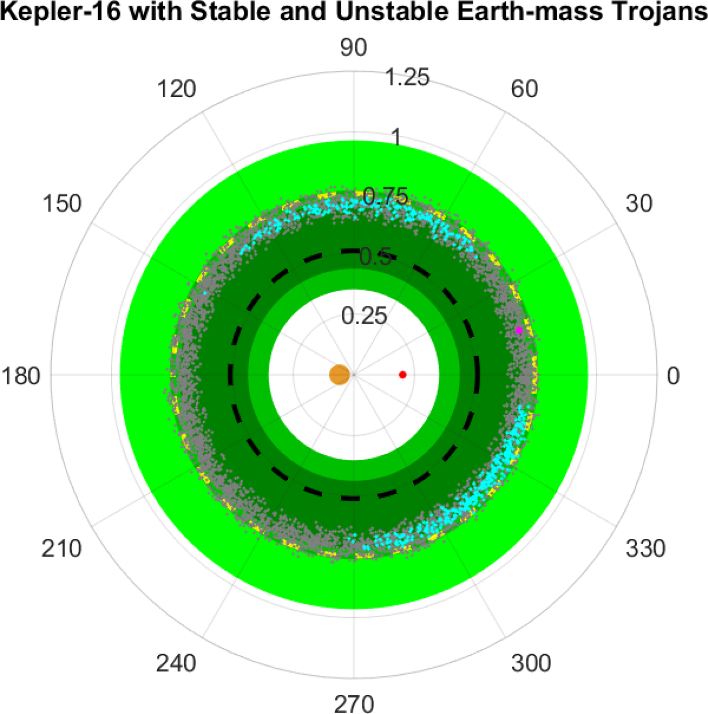
Fig. 10. Illustration of the starting locations of stable (cyan) and unstable (gray) initial conditions out of 5000 trials. These simulations differ from QMC12 as the relative phase between the binary and planetary orbit is now taken into account, where the positive x-axis is taken to be the line-of-sight. See Fig. 7 for information on the colour coding of the HZs.

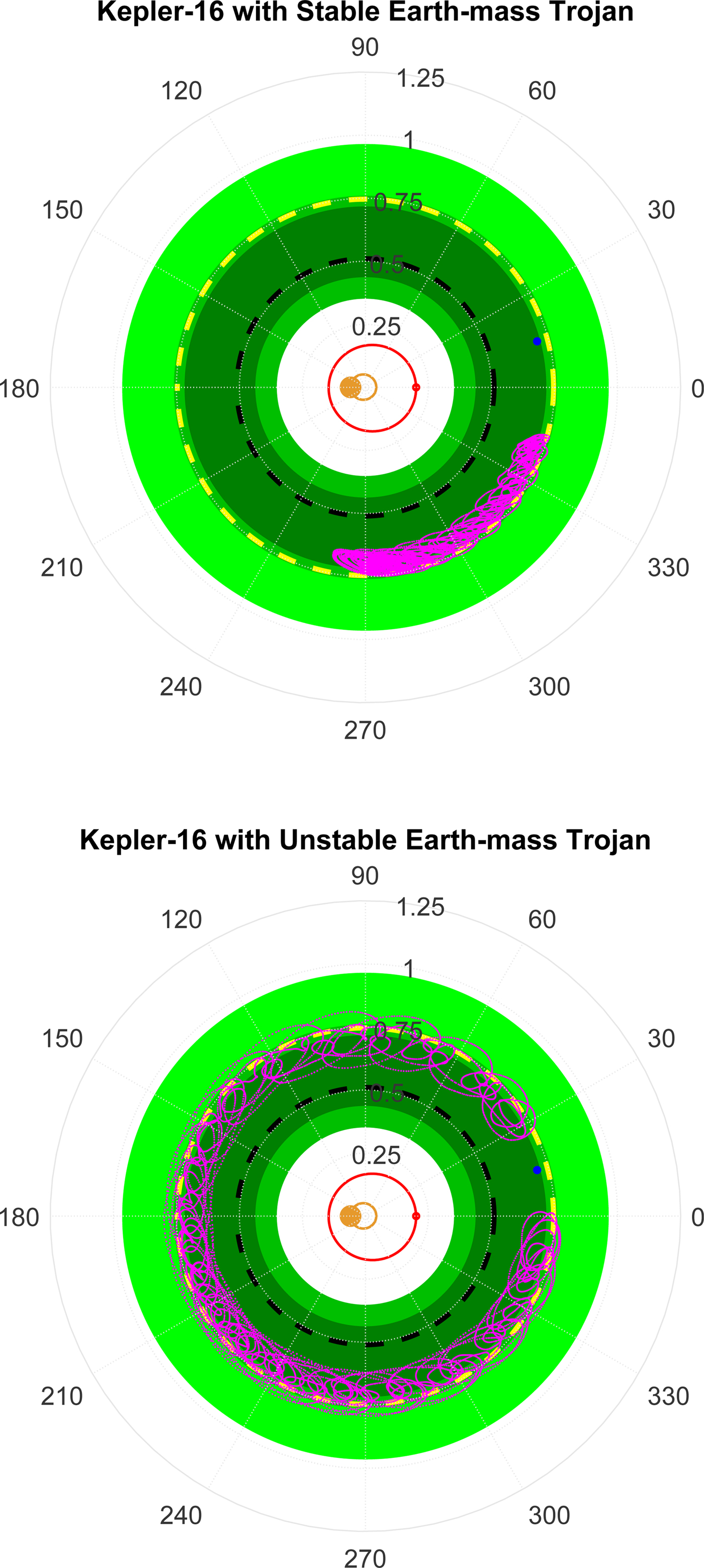
Fig. 11. Examples of orbital evolution (magenta) of a stable (top) and unstable (bottom) Earth-mass planet co-orbiting with Kepler-16b. These orbits are shown in a rotated-reference frame depicting the relative motions with Kepler-16b to illustrate Trojan (top) and horseshoe (bottom) configurations. See Fig. 7 for information on the colour coding of the HZs.

Summary and conclusions

The purpose of our study is to continue investigating the HZ as well as the general possibility of Earth-mass exomoons and Trojans in Kepler-16. The binary system Kepler-16(AB) consists of a low-mass main-sequence star, a red dwarf and a circumbinary Saturnian planet. The temperatures of the two stellar components are given as 4450 ± 150 K and 3308 ± 110 K, respectively. Previously, QMC12 pursued an exploratory study about this system, indicating that based on orbital stability considerations both Earth-mass exomoons and Earth-mass Trojan planets might be possible. The aim of the present study is to offer a more thorough analysis of this system. We found the following results:

1. (1) As previously said by QMC12, Kepler-16 possesses a circumbinary HZ; its width depends on the adopted climate model. Customarily, these HZs are referred to as GHZ and RVEM; the latter is also sometimes referred to as optimistic HZ (e.g., Kopparapu et al., Reference Kopparapu, Ramirez, Kasting, Eymet, Robinson, Mahadevan, Terrien, Domagal-Goldman, Meadows and Deshpande2013; Kaltenegger, Reference Kaltenegger2017). For objects of thick CO₂ atmospheres including clouds, the HZ is assumed to be further extended, thus giving rise to the EHZ as proposed by Mischna et al. (Reference Mischna, Kasting, Pavlov and Freedman2000).

2. (2) Our work confirms earlier simulations by QMC12 that both Earth-mass exomoons and Earth-mass Trojan planets could stably orbit in that system. However, in this study, we adopted longer timescales and also explored the distributions of eccentricity and inclinations of the Earth-mass test objects considered in our study.

3. (3) Exomoons and Trojans, associated with the Saturnian planet, are found to be situated within the lower portion of the EHZ (i.e., ε ≲ 2.2). A more detailed analysis also implies that the distances of those objects may be within the RVEM (i.e., optimistic HZ) if a relatively high luminosity for the stellar components is assumed (but still consistent with the uncertainty bars) or if the objects are allowed to temporarily leave the RVEM-HZ without losing habitability. The latter property is maintained if habitability is provided by a relatively thick atmosphere Williams & Pollard (Reference Williams and Pollard2002).

4. (4) For tutorial reasons, we also compared the HZ of the system's primary to that of the binary system. We found that the latter is reduced by 42% (GHZ) and 48% (RVEM) despite the system's increase in total luminosity given by the M-dwarf. The reason is that for the binary, the RHZ is unbalanced and it is further reduced by the additional requirement of orbital stability as pointed out previously (e.g., Eggl et al., Reference Eggl, Haghighipour and Pilat-Lohinger2013; Cuntz, Reference Cuntz2014).

5. (5) Moreover, we pursued new stability simulations for Earth-mass objects while taking into account more general initial conditions. The attained eccentricity distribution prefers values close to circular, whereas the inclination distribution is relatively flat. The distribution in the initial relative phase indicates that the stable solutions are distributed near the co-orbital Lagrangian points, thus increasing the plausibility for the existence of those objects.

Our study shows that the binary system Kepler-16(AB) has a HZ of notable extent, though smaller than implied by the single-star approach, with its extent critically depending on the assumed climate model for the possible Earth-mass Trojan planet or exomoon. Thus, Kepler-16 should be considered a valuable target for future planetary search missions. Moreover, it is understood that comprehensive studies of habitability should take into account additional forcings by planet host stars, such as stellar activity and strong winds expected to impact planetary conditions as indicated through analyses by, e.g., Lammer (Reference Lammer2007), Tarter et al. (Reference Tarter, Backus, Mancinelli, Aurnou, Backman, Basri, Boss, Clarke, Deming, Doyle, Feigelson, Freund, Grinspoon, Haberle, Hauck, Heath, Henry, Hollingsworth, Joshi, Kilston, Liu, Meikle, Reid, Rothschild, Scalo, Segura, Tang, Tiedje, Turnbull, Walkowicz, Weber and Young2007), Lammer et al. (Reference Lammer, Bredehöft, Coustenis, Coustenis, Khodachenko, Kaltenegger, Grasset, Prieur, Raulin, Ehrenfreund, Yamauchi, Wahlund, Grießmeier, Stangl, Cockell, Kulikov, Grenfell and Rauer2009), Kasting et al. (Reference Kasting, Kopparapu, Ramirez and Harman2014), and Kaltenegger (Reference Kaltenegger2017). Recent articles about the impact on stellar activity on prebiotic environmental conditions have been given by, e.g., Cuntz & Guinan (Reference Cuntz and Guinan2016) and Airapetian et al. (Reference Airapetian, Glocer, Khazanov, Loyd, France, Sojka, Danchi and Liemohn2017).