


Introduction
At present, various approaches to studying life, its emergence and evolution are typically treated with complete coherence; however, the combination of results in a consistent manner has always been a difficult task. It is important not to go further without underlying, what the term chaotic, throughout the present paper stands for. Such behaviour (chaotic) stands for small differences in initial conditions that yield to widely diverged outcomes for such dynamical systems, rendering long-term prediction and repeatability impossible in general (Kellert Reference Kellert1993). A brief review of chaotic behaviours that arise throughout the evolution of the Solar Systems in the Universe, terrestrial planets and planet Earth is presented. The relationships between chaos and the emergence of intelligent life are summarized in (Section ‘Chaotic behaviours, emergence and evolution of intelligent life’). The fact, that the probability of the development of such a scenario approaches zero for every evolution, is demonstrated in the results section based on the stochastic dyadic Cantor set (SDCS) using temporal and spatial randomness.
For more details of chaotic phenomena in planetary formation or the S.D.C.S., I refer the readers directly to the bibliography. In these papers, readers will find more details about the topics and also can have a more in-depth understanding.
Review of chaotic processes in the history of Solar Systems, terrestrial planets and planet Earth
The very first step of planetary formation is the presolar cloud collapse and the formation of the solar nebula. This step inevitably involves a certain amount of stochastic and chaotic evolution (Boss & Goswami Reference Boss, Goswami, Lauretta and McSween2006). In the solar nebula, two mechanisms drive the outflows from the protostar: the X-wind and disc-wind mechanisms (Boss & Goswami Reference Boss, Goswami, Lauretta and McSween2006) where the wind behaviour, evolves into either weak or strong chaos because of the nonlinear Alfvén waves in the solar wind (Horton et al. Reference Horton, Weige and Sprott2001; Chian et al. Reference Chian2007).
The plasma of the central star plasma exhibits multifractal and chaotic behaviour consistent with that of the self-similar generalized weighted Cantor set (Macek Reference Macek2009). In the disc-wind model, the detailed radial structure exhibits a complicated nonlinear behaviour described by the Grad–Shafranov equation (Königl & Pudrtiz Reference Königl, Pudrtiz, Mannings, Boss and Russell2000). A recent finding, has demonstrated some relation between the aftermaths of these plasma and wind behaviours over the course of life evolution. Aftermaths that occurs through the emanation of magnetic fields (Lammer Reference Lammer2013; Park et al. Reference Park, Ryutov, Plechaty, Ross and Kugland2013).
The dust-to-grain formation of planetesimals in solar and extrasolar nebulae is subject to the nonlinear phenomenon of gravitational instability (Chiang & Youdin Reference Chiang and Youdin2010). The sizes of the gaseous circumstellar discs around young stars vary significantly, from tens to thousands of AU (Bbeckwith & Sargent Reference Bbeckwith and Sargent1996; Kretke et al. Reference Kretke, Levison, Buie and Morbidelli2010, Reference Kretke, Levison and Buie2011). From planetesimal to protoplanets two regimes appears, the dispersion-dominated and Keplerian shear regimes (Rafikov Reference Rafikov2004). The disc-accretion turbulence, such as that of magnetohydrodynamics (MHD), applies in this stage of evolution, exerting effects on the solar nebula and, by extension, the protostellar and protoplanetary discs (Balbus & Hawley Reference Balbus and Hawley2000). MHD turbulence is not a nonlinear outcome of the instability, but rather is the essence of the instability (Balbus & Hawley Reference Balbus and Hawley2000). Also, in this stage, the dynamical evolution of the dispersion-dominated regime produces chaotic orbits as a result of multiple scattering (Rafikov & Slepian Reference Rafikov and Slepian2010).
Planetary migration progresses through significantly nonlinear mechanisms. The most fundamental recent change in the understanding of planetary-system formation was the realization that the planets may not have formed in the orbits in which we now observe them (Rafikov & Slepian Reference Rafikov and Slepian2010). Planetary migration is not as simple as the adiabatic model predicts, if the resonance is surrounded by a chaotic layer, as is the case, if the planet's eccentricity is not zero or if the inclination of the particle is large; in fact, the technique is essentially impossible to apply in such a case because it also depends on the diffusion speed inside the chaotic layer (Levison et al. Reference Levison, Morbidelli, Gomes, Backman, Reipurth, Jewitt and Keil2007). The giant planets suffered significant radial migration in the early history of our Solar System (Malhorta Reference Malhorta1998). The migration of the giant planets perturbed the planetesimal disc, where later the terrestrial zone of the Solar System suffered a period of considerable bombardment (Hahn & Malhorta Reference Hahn and Malhorta1998). High-mass planets such as Jupiter induce a nonlinear disc response (Szuszkiewicz & Papaloizou Reference Szuszkiewicz and Papaloizou2010) during their transit. It is likely that the mutual interactions of planets during resonant crossings influence their subsequent evolution, while remaining either close to or within the chaotic regime (Papaloizou & Szuszkiewicz Reference Papaloizou and Szuszkiewicz2005). MHD instabilities are robust; migration will generally proceed in a highly chaotic manner (Laughlin et al. Reference Laughlin, Steinacker and Adams2004; McNeil & Duncan Reference McNeil and Duncan2005). The passage of a migrating planet through a swarm of smaller planetesimals is a transitory event with long-term consequences (Lufkin et al. Reference Lufkin, Richardson and Mundy2006). The subsequent step is the completion of the oligarchic growth of planetesimals that leads to chaotic growth (Nagasawa et al. Reference Nagasawa, Thommes, Kenyon, Bromley, Lin, Reipurth, Jewitt and Keil2007). As they accumulate from planetesimals into protoplanets, the oligarchic planets, which are in roughly circular orbits, evolve into a chaotic system and begin to collide (Nagasawa et al. Reference Nagasawa, Thommes, Kenyon, Bromley, Lin, Reipurth, Jewitt and Keil2007).
The water contents, composition and configurations out of these giant collisions are highly variable (Nagasawa et al. Reference Nagasawa, Thommes, Kenyon, Bromley, Lin, Reipurth, Jewitt and Keil2007) because the habitability of a planet is strongly affected by the impacts of comets and asteroids (Booth et al. Reference Booth, Wyatt, Morbidelli, Moro-Martín, Levison, du Foresto, Gelino and Ribas2009). The large dimensionality of the system, the long-range interactions, and the complexity of the dynamics at this stage, mean that these giant impacts and collisions are a source of chaos that is only limitedly understood (Diacu & Holmes Reference Diacu and Holmes1997; Gomes et al. Reference Gomes, Levison, Tsiganis and Morbidelli2005). The late stage of planetary formation is of particular importance; it is during this period that the mass, spacing and spin angular momentum of the planets are finalized and the presence of impact-generated satellites arises (Agnor Reference Agnor1999).
Chaos arises in systems with many degrees of freedom (Beaugé et al. Reference Beaugé, Callegari, Ferraz-Mello and Michtchenko2005). In the current Solar System, there is chaotic evolution (Sussman & Wisdom Reference Sussman and Wisdom1992), and large-scale chaos (Laskar Reference Laskar1994). The most immediate expression of this chaotic behaviour is the exponential divergence of trajectories with similar initial conditions (Laskar Reference Laskar2003). The Earth may experience a large chaotic zone from 0° to 85° in its obliquity (Laskar Reference Laskar2003). However, the Moon causes the Earth to vary no more than 1.3°–23.3° in obliquity (Laskar Reference Laskar2003), already inducing significant changes in insolation over the Earth's surface. The outer Solar System exhibits chaotic behaviour (Haynes Reference Haynes2007), and Pluto presents its own chaotic pattern (Sussman & Wisdom Reference Sussman and Wisdom1998). The spacing of the inner planets in the Solar System exhibits large-scale chaos (Laskar Reference Laskar1997). The most representative and frequent chaotic interaction of the Earth is reflected by the fact that without the Moon, the Earth would experience variations in its obliquity with high probability (Néron de Surgy & Laskar Reference Néron de Surgy and Laskar1997). The Moon stabilizes the Earth's obliquity, and hence, the variations in insolation on its surface (Laskar & Robutel Reference Laskar and Robutel1993).
Chaotic behaviours, emergence and evolution of intelligent life
When considered in terms of the generalities and constants of chaotic nonlinear behaviours (Feigenbaum Reference Feigenbaum1983), each human being represents a unique occurrence in the history of mankind, just as the creation of any given planet represents a unique occurrence in the history of the Universe, with unique and differentiating characteristics at all possible scales (Iovane et al. Reference Iovane, Laserra and Tortoriello2004; Ispolatov & Doebeli Reference Ispolatov and Doebeli2014). Each planet, such as planet Earth represents the appearance of a particular outcome in the Universe at the stochastic, self-similar and fractal levels (Iovane et al. Reference Iovane, Laserra and Tortoriello2004). The continuous link between nonlinear chaotic behaviours throughout planetary formation and chaotic behaviours in the evolution of life, exist through evolutionary dynamics. Evolutionary chaos is indeed common, and unpredictability is the rule rather than the exception (Ispolatov & Doebeli Reference Ispolatov and Doebeli2014). In the case of mankind, this particular outcome represents a universal system of nonlinear chaotic behaviours interacting through exact adjustments, sequences, processes, and deterministic and stochastic behaviours, to ensure the habitat, emergence (Ispolatov & Doebeli Reference Ispolatov and Doebeli2014) and evolution of life; specifically, intelligent life, on Earth (Walker et al. Reference Walker, Cisneros and Davies2012).
The required theoretical circumstances, in which the evolution of a planet with intelligent life in the universe can occur, for observational purposes, are described by the evolution of the protoplanetary cloud (Safronov Reference Safronov1967). However, this provides only a deterministic structure. The actual process proceeds through four loosely defined stages (Lissauer & Stewart Reference Lissauer, Stewart, Levy and Lunine1993): the initial stage, the early stage, the middle stage and the late stage. Throughout the introductory review section, the relationships among the chaotic behaviours in these four stages have been presented. To track each occurrence, N-body simulations are required to calculate the nonlinear final states of the actual theories of structure formation (Lake et al. Reference Lake, Quinn and Richardson1997). An N-body simulation implies the modelling of the interactions of multiple particles in a chaotic system, where determinism guides the evolution of the system from conservative to non-conservative (Lake et al. Reference Lake, Quinn and Richardson1997). Determinism leads to chaos (Hadjidemetriou & Voyatzis Reference Hadjidemetriou and Voyatzis2011). If chaotic dynamics are followed or repeated many times, then each time, they will yield a result that differs from previous results in all its microscopic and macroscopic components (Kellert Reference Kellert1993). Chaotic behaviours may serve to satisfy general expectations, but cannot be guaranteed to produce any particular outcome. Observational data from more than 250 planetary systems exhibit a wide range of different masses, orbits and, in multiple systems, dynamical interactions (Thommes et al. Reference Thommes, Matsumura and Rasio2008). The results of the Kepler mission indicate that nearly 17 billion Earth-like planets exist in the Milky Way (Harvard-Smithsonian Center for Astrophysicist), suggesting different past evolution and formation scenarios with highly similar initial conditions. The discoveries by Spritzer, Hubble, Keck and Kepler of multiple Earth-like planets, or the studies of pre-RNA chemical evolution and the organic material back to the earliest epochs of Galaxy formation, demonstrates the stunning similar processes that were, are or will be at work in the Universe. These processes represent an exponential divergence of similar initial evolutions into universal and observable large-scale differences that affect the overall generation and sustainability of intelligent life (Martinez & Bernard Reference Martinez and Bernard1990; Pesin & Weiss Reference Pesin and Weiss1997; Iovane et al. Reference Iovane, Laserra and Tortoriello2004; Radburn-Smith et al. Reference Radburn-Smith, Lucey, Woudt, Kraan-Korteweg and Watson2006; Thommes et al. Reference Thommes, Matsumura and Rasio2008; Argón-Calvo et al. Reference Argón-Calvo, Weygaert and Jones2010; Walker et al. Reference Walker, Cisneros and Davies2012; Ispolatov & Doebeli Reference Ispolatov and Doebeli2014). The evolutionary processes of such systems will not proceed through any exact sequence to produce one particular, detailed and fine-tuned outcome. Even with intentional planning, it would be difficult, if not impossible, to ensure that conditions that would trigger the evolution of intelligent life would arise, by virtue of the sensitive dependence on initial conditions of the related dynamics (Kellert Reference Kellert1993; Iovane et al. Reference Iovane, Laserra and Tortoriello2004; Ispolatov & Doebeli Reference Ispolatov and Doebeli2014). Although, the range of possibilities possesses wide changes through certain similar limits, all arrangements are impossible to duplicate, repeat, forecast or predict into any chaotic behaviour (Kellert Reference Kellert1993).
The intelligent life evolution pattern (based on carbon, DNA–RNA–protein), is an emergent event of the system, that occurs through the course of evolutionary chaos, rather than an event imposed on the system by external influences (Ispolatov & Doebeli Reference Ispolatov and Doebeli2014).
A life evolution pattern with evolutionary chaos (Ispolatov & Doebeli Reference Ispolatov and Doebeli2014) encompasses with the chaotic evolution of terrestrial planets. The precise evolution required for this outcome has a particular cosmological and universal fingerprint that marks mankind, as intelligent life, as unique at all possible scales in the Universe (Kellert Reference Kellert1993; Iovane et al. Reference Iovane, Laserra and Tortoriello2004).
Method
At present, numerical approaches are calculated by combining the quantity or probability of some factors or processes that are required to develop and sustain any sort of life. However, there is no time dependence or the possibility to incorporate into the factors, the physico-chemical history of the Galaxy in the current formulae. As an example, the terrestrial genetic code existed even before the Earth scenario (shCherbak & Makukov Reference shCherbak and Makukov2013), with the necessary precise tuning of all requirements for a life-supporting terrestrial planet, arose.
The formulae for better precision require to accounting spatiotemporal influence, nature's freedom and the effects of any evolutionary process, topics that have not been completely involve. The S.D.C.S. identifies the probability path of any terrestrial planetary formation, involving carefully, time dependence, spatial (probability) influence, nature's freedom in the selection process and randomness (Hassan et al. Reference Hassan, Pavel and Kurths2014). Fractals in nature appear through time evolution and nature is governed by a sort of randomness. Nature does not like determinism; rather it likes to enjoy freedom in the selection process and in the present context freedom means the liberty to divide an interval randomly at any time (Hassan et al. Reference Hassan, Pavel and Kurths2014). The S.D.C.S. divides an interval randomly into two smaller intervals that are not equal in size. This framework provides the inclusion of spatiotemporal effects with randomness, time dependence and the possibility to incorporate into the factors, physico-chemical history through probability.
Components:
• An initial analysis may start with the protoplanetary cloud (Safronov Reference Safronov1967) or the first stage of planetary formation (Lissauer & Stewart Reference Lissauer, Stewart, Levy and Lunine1993) to avoid any uncorrelated or fallacious trajectories with unphysical paths that are not relevant or do not exist for terrestrial planetary formation and the emergence of intelligent life.
• The iterative process may involve infinite values for different time intervals, where (t) is a range of time in which P remains constant. At a certain x value for t, where t is either a discrete or continuous variable through the iteration of the algorithm, (P Life) represents the probability of achieving or maintaining the precise characteristics necessary to support life, higher life forms or intelligent life.
• The common x values for t (time intervals), represent high probabilities for terrestrial planetary-life evolution. In the simplest case of mere naked-eye inspection, it appears that many planets could be capable of sustaining life. Moreover, with only an initial x 1 value for t; with x 1 = 0 it is possible to suppose that in the absence of any iteration, there might be life, higher life forms or intelligent life everywhere, as P = 1.
• All possible processes of terrestrial planetary-life evolution at an x value for t (time interval), during the process of iteration, will have a probability (P) of success.
• With enough x values for t (time intervals) and probabilities, we will achieve a precise description of the terrestrial planetary-life probability path (P Life). These x values for t (time intervals) will precisely model the multiple changes and different characteristics observed for each planet over time (Thommes et al. Reference Thommes, Matsumura and Rasio2008).
Stochastic–probabilistic:
• An a posteriori probability arises, as not all terrestrial planetary formations have occurred. The probability can thus be divided into (P) and (1 − P) within the degrees of freedom and randomness provided by nature. The (1 − P) interval is removed, as it represents the failure of any one of the precise characteristics of the terrestrial planetary formations that are required for any sort of life to emerge and evolve.
Self-similar:
• The self-similar property allows on each iteration, a range of probabilities of (0, 1]. Without this property, the range of probabilities for every new occurrence or iteration will be starting with a shorter probability of (1 − P) from the previous range of P.
Fractal:
• Through the S.D.C.S., fractal geometry gives the most detailed and ad infinitum precision accounting the importance of any factor at work through any scale (microscopic–macroscopic).
Chaotic:
Chaotic behaviours extensively modify the probability of each terrestrial planetary formation, as they could cause a given scenario to fail or to maintain the precise characteristics necessary to support life, higher life forms or intelligent life.
The stochastic dyadic Cantor set (S.D.C.S.) with temporal and spatial randomness, exhibits ad infinitum behaviour with a probability distribution on R″ that is concentrated on a set of Lebesgue measure zero. In other words, a probability that tends to zero is assigned to every single point in the set, such as the point that corresponds to the particular and unique life forms we would like to find.
The probability path (P Life) starts with any terrestrial planetary formation, evolving until it reaches its particular and unique configuration.
Figure 1 illustrates the iterative process of identifying the exact probability path for a specific type of terrestrial planetary-life formation.

Fig. 1. Identifying an exact probability path using the S.D.C.S.
Through the self-similar and fractal properties on each step of iteration (Hassan et al. Reference Hassan, Pavel and Kurths2014), the algorithm presents necessarily, a dimensional analysis that would also rise to the conclusion that generalities, may rise the expectations to the fact that intelligent life would exist. However, Fig. 2 illustrates the example of the precise path required, for the expectation of intelligent life appearance.
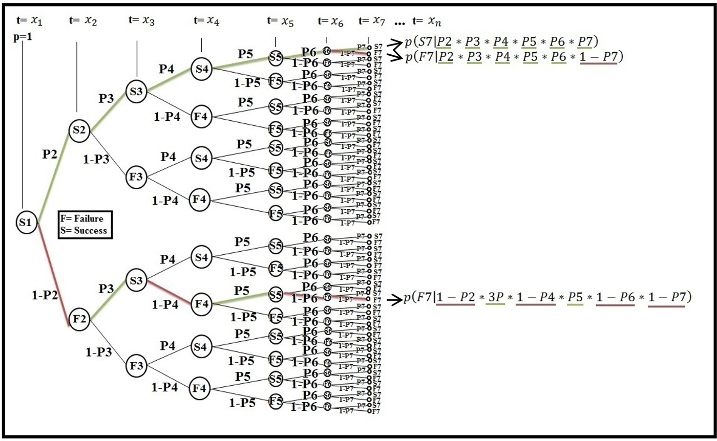
Fig. 2. Identifying exact probability paths through the S.D.C.S. using a probability tree.
The method can be applied by incorporating any evolutionary history of terrestrial planetary formation in the Universe within a set of stochastic, self-similar and fractal (Hassan et al. Reference Hassan, Pavel and Kurths2014) dimensions. The precise probability path (P Life) for one particular evolutionary history of terrestrial planetary life will be produced through the iterative process of successes.
Figure 2 illustrates, through a probability tree, how the stochastic dyadic Cantor set with temporal and spatial randomness can be applied to generate all possible probability paths for each evolutionary history of terrestrial planetary formation in the Universe. The figure also illustrates the statistical self-similarity behaviour at each step of iteration. It is important to note that here the (1 − P) is removed from the S.D.C.S. leading to the uniqueness of any evolution sequence with each occurrence. However, each planet in the Universe continues to evolve as part of the sample space regardless of whether it can support life, higher life forms or intelligent life. Each probability path (P Life) is the result of all possible combined probabilities that have appeared throughout the path prior to that point, but on a stochastic, self-similar and fractal scale (Iovane et al. Reference Iovane, Laserra and Tortoriello2004). Each probability path (P Life) approaches zero because it depends on all possible combined events that may occur before the capability of supporting complex life emerges. Figure 2 also presents three particular probabilistic paths (P Life) that could occur during terrestrial planetary formation. It is important not to forget that for t = x 1, with x 1 = 0; P = 1.
What follows is an explanation of three short sequences out of the infinite probabilistic paths (P Life) that could be depicted by continuing the iterating process in Fig. 2:
p(S7|P2*P3*P4*P5*P6*P7): Represents a unique probability path for a planet to support life, higher life forms or intelligent life, as in the case of planet Earth. It illustrates the precision necessary to achieve fine-tuned requirements through enough iteration to the microscopic and macroscopic scales.
p(F7|P2*P3*P4*P5*P6*1 − P7): Represents a type of outcome, in which there is some number of successes and perhaps, few failures of a requirement for a terrestrial planetary formation to support life, higher life forms or intelligent life.
p(F7|1 − P2*3P*1 − P4*P5*1 − P6*1 − P7): Represents a type of outcome, in which there is some number of successes but many failures of various requirements for a terrestrial planetary formation to support life, higher life forms or intelligent life.
What follows, is the formulae for better precision, to identify the probability path of any terrestrial planetary formation to support life, higher life forms or intelligent life through the S.D.C.S. The present formula accounts the importance of spatiotemporal influence, nature's freedom and the effects of any evolutionary process, topics that have not been completely involve in current formulae. It is convenient to introduce two variables defined as follow:
 $$\left\{ {\matrix{ {P\; ;\;{\rm with}\;\; 0 \lt P \le 1} \cr {t;\;{\rm with\;} \;t \ge 0} \cr},} \right.$$
Pt, represents through an interval of time, the probability of each process, known or unknown, that did occur, is occurring or will occur within this framework of self-similar, stochastic, fractal and chaotic behaviours (Kellert Reference Kellert1993; Iovane et al. Reference Iovane, Laserra and Tortoriello2004; Ispolatov & Doebeli Reference Ispolatov and Doebeli2014); where t (time interval) is a range of time in which P remains constant. In other words, the constant probability of each process (P) will have a time dependence (Pt) in that interval of time (t), where it will be achieved or maintained through the iteration of the algorithm (∏t≥0Pt) the precise characteristics and probability (P Life) to support life, higher life forms or intelligent life on a particular planet
 $$P_{{\rm Life}} = \mathop \prod \limits_{t \ge 0} P^t. $$
Seemingly, there could be a number of trajectories belonging to a subset that produces intelligent creatures with similar attributes and faculties. Also, at first glance, the iterations of short time intervals produce high probabilities for those trajectories of planetary life existence; however, the final outcome is only possible if all arrangements are precisely tuned through enough iterations with the right ranges for every time interval (t). Life vanishes on each iteration, on each change. All outcomes will become unique while evolving. The range of possibilities possesses wide changes through certain similar limits, where all arrangements are impossible to duplicate, forecast or predict into any chaotic behaviour (Kellert Reference Kellert1993).
The following figures illustrate the numerical simulation of the formula, to identify the probability path of any terrestrial planetary formation and the emergence–evolution of intelligent life through the S.D.C.S. For the iterations of one million years (1.0 Myr), the numerical simulation stands for the convention of (1.0 Myr = 106) value, hundred thousand years (0.1 Myr), ten thousand years (0.01 Myr) and so forth. Hence, identifying the probabilities during various ranges of time, of different terrestrial planetary formations and Solar Systems (Montmerle et al. Reference Montmerle, Augereau, Chaussidon, Gounelle, Marty and Morbidelly2006) also, there it is no repeatability of probabilities, since chaotic nonlinear behaviours are at work. Figs. 3(a, b), 4(a, b) and 5 repeat on each iteration a P of (0.99) intentionally, for the purpose of exemplifying, how complex the behaviour of the simulation evolves on Figs 6–9 with, more iterations, ranges of time and a (0, 1] range of probabilities for any event. The algorithm accounts the importance of any interval of time (billion, million and thousand years), thus avoiding insufficient representation of any event and its chorological occurrence into any interval of time. Finally Table 1 shows the tendency to zero for five different sequences.

Fig. 3. Changes through short time intervals over periods of thousand years, with overvalue and constant probabilities that would yield to the fact of complex life emerge (P = 0.99): (a) When considering the entire range of P, P Life exhibits high probabilities; (b) When the range of P, is adjusted, P Life shows how vanishes on each iteration.

Fig. 4. Changes through short time intervals (million years) with overvalue and constant probabilities that would yield to the fact of complex life emerges (P = 0.99): (a) When considering the entire range of P, P Life exhibits through 10 millions of years, its small decreasing probability; (b) When the range of P, is adjusted, P Life shows how vanishes on each iteration.

Fig. 5. When considering the entire range of P, even with an overvalued P = 0.99 of success on each iteration and assuming that P would remain constant over every hundred millions of years, P Life now exhibits through 4.5 billions of years, its decreasing probability behaviour, that approaches zero into the first 200 millions of years.

Fig. 6. With random probabilities; with 0.5 ≤ P ≤ 1, through 45 iterations, P Life exhibits its tendency to zero. The probability path (P Life) approaches zero in the first 14 changes or 14 iterations.

Fig. 7. With random probabilities; with 0.5 ≤ P ≤ 1, the iteration now exhibits through 4.5 billions of years, its tendency to zero over a time interval (t) of 10 million years. In other words, assuming that P would remain constant and iterated through every 10 million years; with 0.5 ≤ P ≤ 1, the probability path approaches zero into the first 120 millions of years.

Fig. 8. With random probabilities; even with 0.5 ≤ P ≤ 1, the iteration now exhibits through 4.5 billions of years, its tendency to zero over a time interval (t) of million years. In other words, assuming that P would remain constant and iterated through every million years; with 0.5 ≤ P ≤ 1, the probability path approaches zero into the first 10 millions of years.

Fig. 9. Random changes every ten thousand years, over a period of 150 millions of years, with random P values; with 0.001 ≤ P ≤ 1, and random (t) values; with 0 ≤ t ≤ 0.01, P Life exhibits through 150 millions of years, its tendency to zero, where P Life approaches zero into the first 5 millions of years. The exponential equation for this particular P Life appears in the figure.
Table 1. First iterations for five different terrestrial evolution sequences (probability paths) with random changes every ten thousand years, with random P values; with 0.001 ≤ P ≤ 1 and random (t) values; with 0 ≤ t ≤0.01

Notes These first steps of iteration exhibit the property of similar conditions while evolving, with a tendency to zero. The probability path (P Life) approaches zero right after the very first 5 millions of years, where precise characteristics are crucially necessary to support intelligent life, its emergence, and evolution. Also, the rich behaviour of these paths as a property that emerges from the evolution sequence rather than one that emerges from external influences.
Through a numerical example, even with overvalue and constant probabilities that would yield to the fact of complex life emerges (P = 0.99), the S.D.C.S. approaches zero after five hundred consecutive values for t (million years); where the probability of life, higher life forms or intelligent life, vanishes on each change.
 $$P_{{\rm life}} \left( {\left. {P^t} \right \vert 0.99{^\ast}0.99{^\ast}0.99{^\ast}0.99^{497}} \right) = 6.570483 \times 10^{ - 3}.$$
It is important to note the following condition, because with (P = 0.5), through seven iterations, life vanishes significantly faster.
 $$P_{{\rm Life}} \left( {\left. {P^t} \right \vert 0.5^7} \right) = 7.8125 \times 10^{ - 3}. $$
Although it seems at first glance that iterations of short-time intervals, produce high probabilities of the existence of planetary life existence, this outcome is only possible if all arrangements are precisely tuned through enough iterations with the right ranges for every time interval (t); and however, on each iteration, on each change, P Life vanishes.
Through the course of various simulations, the tendency to zero is an invariant behaviour that appears for different values for t (time interval). Also, innumerable changes occur through a chaotic system and decadal to billion years cycles in astronomical, biological, climatic, geomagnetic, solar, volcanic and genetic occurrences (Puertz et al. Reference Puertz, Prokoph, Borchardt and Mason2014). The tendency to zero is the result of all possible combined probabilities of all occurrences that have appeared throughout the path prior to the point of finding intelligent life. The following figures (Fig. 10(a) and (b)) depict two scenarios, where, it is exhibited how fast or slow the tendency approaches zero with probabilities; 0.01 ≤ P ≤ 1 and 0.99 ≤ P ≤ 1.

Fig. 10. (a) Changes; with 0.01 ≤ P ≤ 1, where, P Life exhibits its tendency to zero. The probability path (P Life) approaches zero over the first seven changes; (b) Changes; with 0.99 ≤ P ≤ 1, which would yield to the fact of complex life emerges, P Life exhibits its tendency to zero over 500 iterations. The probability path (P Life) approaches zero over 500 changes.
It is important not to forget that a method to find the randomness of an event, consists on many trials that will give out its frequency, or its probability of occurrence. If only a single result appears through enough trials, then, the nature of the event should be deterministic; therefore, not going further with a longer sequence of trials to find out its probability of occurrence. In the present context, two events occurred. Event one, it is to find through chaotic dynamics the probability of the existence of intelligent life throughout the Universe. Event two, it is to find intelligent life on earth. As demonstrated, the probability of the occurrence of event one, on all trials in the Universe including earth, tends to zero. All trials will exhibit the different results of deterministic, stochastic and chaotic behaviours influencing the entire dynamics through billions of years. However, for the second event, to find intelligent life on Earth, the result is being assumed as deterministic, not taking into account the many probabilistic behaviours and chaotic dynamics into it. Thus, the chance of finding intelligent life on earth is at least equal to one, unless affirming or changing the result, through enough trials carried out particularly on earth. Chaotic dynamics combine deterministic and stochastic behaviours through time. Another term for chaos it is deterministic chaos, and its meaning represents a stochastic behaviour into a deterministic system. The formation of planet Earth consisted of all kinds of behaviours, deterministic and probabilistic, such as quantum, atomic and photonic processes, among many others. However, as said above, evolutionary chaos renders unpredictability and non-repentance through the course of planetary formation and the evolution of intelligent life (Kellert Reference Kellert1993; Ispolatov & Doebeli Reference Ispolatov and Doebeli2014). It is important to note that here, it is not about the processes that render a planet inhabited or uninhabited. It is about the dynamics and how each entire sequence with its processes approaches zero and emerges unique while evolving.
Theory
The evolution of any sort of life can be divided into chronological intervals in which different behaviours appear. It is not possible to predict any specific expected outcome for any chaotic event (Kellert Reference Kellert1993). All outcomes will be different and play unique roles in the sequence of events. Moreover, chaotic behaviours (Feigenbaum Reference Feigenbaum1983; Kellert Reference Kellert1993; Ispolatov & Doebeli Reference Ispolatov and Doebeli2014) generally arise in the stochastic, self-similar and fractal (Iovane et al. Reference Iovane, Laserra and Tortoriello2004) dimensions of terrestrial planetary-life evolution throughout the Universe. The intelligent life evolution pattern (based on carbon, DNA–RNA–protein), is an emergent event of the system, that occurs through the course of evolutionary chaos, rather than an event imposed on the system by external influences (Ispolatov & Doebeli Reference Ispolatov and Doebeli2014). Chaotic behaviours extensively modify the probability of each terrestrial planetary formation, as they could cause a given scenario to fail or to maintain the precise characteristics necessary to support life, higher life forms or intelligent life. Even with the necessary and sufficient conditions across multiple sites and epochs in the history of the Universe. The entire pattern of the sequence proceeds through an exact path of probabilities (P Life) in a fractal behaviour that is revealed by the entire evolution sequence, which encompasses processes with statistically self-similar behaviour at every scale. Thus, the S.D.C.S. exhibits the rich behaviour of this path as a property that emerges from the evolution sequence rather than one that emerges from external influences, as sensitive dependence is constantly modifying the outcome (Kellert Reference Kellert1993). All outcomes will become unique while evolving.
To construct such a path (P Life) for every possibility, it requires a perfect set in topology, with self-similar iterations and the capability of providing different probabilities over time. The required set should be able to model the probability-formation path of every planet in the Universe and should account for the successes or failures of precise characteristics for the emergence and evolution of terrestrial planetary life. Specifically, the S.D.C.S. with temporal and spatial randomness (Hassan et al. Reference Hassan, Pavel and Kurths2014) possesses the characteristics that are required: an infinite number of intervals; infinitesimal size; existence near any point that belongs to the set itself; and a generating function with fractal properties on a [0, 1] interval that is not absolutely continuous and is compact, totally disconnected, perfect (every point is an accumulation point) and uncountable. This function provides a one-dimensional interval for calculating the sequential path of probabilities of every terrestrial planetary-life evolution in the Universe.
The S.D.C.S. with temporal and spatial randomness, manifest through probability, the intrinsic chaotic effects over the course of emergence–evolution of any kind of life in the Universe. Both, simplistic but complex, the model accounts the importance of infinite possible paths, temporality with infinite continuous or discrete variables and infinite choices over the entire set of sufficient iterations to observe each planet and life, with their unique characteristics and particular probabilities. The S.D.C.S. with temporal and spatial randomness, models the stochastic, self-similar and fractal characteristics consistent with those of the stochastic, self-similar and fractal dimensions of the Universe (Iovane et al. Reference Iovane, Laserra and Tortoriello2004; Hassan et al. Reference Hassan, Pavel and Kurths2014). With a single iteration, the S.D.C.S. with temporal and spatial randomness manifests the straightforward argument from probability theory, of a simple binary choice with probability P. However, with more than one iteration, a binomial model is not continuous and precise, since P must change on every iteration, because nonlinear chaotic behaviours render long-term prediction and repeatability impossible in general (Kellert Reference Kellert1993).
An absolutely discrete model such as binomial or a single binary choice will not model: stochastic, self-similar, fractal, deterministic, probabilistic, chaotic, discrete and continuous behaviours throughout the Universe for the probability of finding intelligent life.
It is important to remark that all outcomes through the S.D.C.S. with temporal and spatial randomness are just as unique and desirable such as planet Earth and intelligent life.
Consequently, to avoid the common mistake of confounding probability after the fact, with probability before the fact and the so common nil and extremely low probabilities after the fact; as said above, the terrestrial genetic code (DNA) existed even before the fact of Earth's scenario (shCherbak & Makukov Reference shCherbak and Makukov2013), with the necessary precise tuning of all requirements for a life-supporting terrestrial planet, arose. Even, the intelligent life evolution's pattern (based on carbon, DNA–RNA–protein), is an emergent event of the system, that occurs through the course of evolutionary chaos, rather than the fact of imposed events on the system, by external influences (Ispolatov & Doebeli Reference Ispolatov and Doebeli2014).
In contrast, it is driving to prove to consider that a probability model for the appearance of life, behaves analogously to going as many times possible to a casino, and bet all chips on every throw of the dice. Going broke is a fact.
Finally, the mechanism of the evolution of the protoplanetary cloud (Safronov Reference Safronov1967) implies that the process of planetary formation occurs throughout the Universe, not only for particular planets. Through all processes that arise during planetary formation, (P Life), of any sort of life will appear as an emergent property with two primary, dichotomous characteristics:
• The (P Life) pattern appears with exact and precise arrangements through the micro–macro levels.
• Such an expected (P Life) pattern will occur only through sensitive dependence on the initial conditions that will enable the necessary unique characteristics to arise, as exact precision is required. Enough iterations are needed to produce such an uncommon, fine-tuned outcome, out of chaotic events.
Results
The unique relationships on Earth among the factors that are required for a terrestrial planet to support life over time are precisely organized into micro–macro interactions and relations. The terrestrial genetic code existed even before the Earth scenario (shCherbak & Makukov Reference shCherbak and Makukov2013), with the necessary precise tuning of all requirements for a life-supporting terrestrial planet, arose; aside from the general occurrence of the nonlinear chaotic behaviours discussed in the introduction, no particular exact arrangement of processes and their interactions is ever repeated or forecast. In the process of the development of terrestrial planets, just one event is known so far to have produced and maintained life, higher life forms and intelligent life; the Earth. The Earth also represents the required, unique and non-repeatable evolution pattern or probability path (P Life), for the emergence and evolution of any sort of life, with a tendency to a Lebesgue measure zero.
Thus, by virtue of the S.D.C.S. with temporal and spatial randomness iterated to the exact precision necessary for mankind's existence, the probability of mankind's existence or intelligent life can be shown to be that tends to zero.
Further developments
It has been suggested that formation and migration may occur simultaneously (Lufkin et al. Reference Lufkin, Richardson and Mundy2006). The time ranges in which this may occur fall within the ranges that correspond to the Keplerian and dispersion regimes (Rafikov Reference Rafikov2004). Thus, terrestrial planetary formation and the evolution of life could be affected not only by chaotic behaviours, but also by the immediate influences and more subtle effects of riddled basins of attraction (Kapitaniak Reference Kapitaniak, Maistrenko, Stefanski and Brindley1998).
Discussion
At present, there is a bias towards time intervals with short or long ranges of time to estimate the existence of life, complex life or intelligent life. Also, constant probabilities for those ranges of time, where few time intervals and probabilities increase significantly the possibilities to find life, complex life or intelligent life. Although it seems at first glance that time intervals and iterations produce high probabilities of the existence of planetary life existence, this outcome is only possible if all arrangements are precisely tuned through enough iterations with the right ranges for every time interval (t) and however, on each iteration complex life vanishes. The range of possibilities possesses wide changes through certain similar limits, where all arrangements are impossible to duplicate, forecast or predict into any chaotic behaviour (Kellert Reference Kellert1993). Thus, from the perspective of nonlinear chaotic behaviours, every planet in the Universe, as in the case of planet Earth, are samples of an ongoing and unique evolution. It is understood that the entire sequence of this evolution is necessary for the existence of intelligent life. The evolution of a protoplanetary cloud (Safronov Reference Safronov1967), a deterministic structure, is followed by many probabilistic and deterministic stages. Moreover, the evolution sequence undergoes critical processes in chaotic phases, which define and determine the emergence, sustainability and evolution of intelligent life or, indeed, any sort of life. Many different results can arise from the chaotic nature and interactions of these events. Even, the intelligent life evolution pattern, based on carbon, DNA–RNA–protein, will differ from all possible sequences. The influence of chaotic behaviours and, perhaps, riddled basins of attraction (Lufkin et al. Reference Lufkin, Richardson and Mundy2006; Kapitaniak Reference Kapitaniak, Maistrenko, Stefanski and Brindley1998) represents a one element among a variety of physical and biological mechanisms that are necessary to produce life, higher life forms or intelligent life. Chaos as an important factor in differentiating the results of each trial: without the differentiation of results from each trial, there would be only a single deterministic outcome with no variations, with a probability of P = 1, giving rise to the Fermi paradox. It is important to mention that the uniqueness of life, from other authors such as (Tipler Reference Tipler1980) was already claimed, arguing that extra-terrestrial begins do not exist (Puertz et al. Reference Puertz, Prokoph, Borchardt and Mason2014).
One concise and paradoxical conclusion appears. The probability of the existence of intelligent life in the Universe tends always to zero. Even the expected probability of repetition is zero. We cannot know exactly the precise path of evolution that mankind followed, although we may know some of the most basic requirements. Mankind is extremely unique, uncommon, alone and irreproducible, given the known or unknown processes that were, are or will be at work in the Universe, as demonstrated by the iterative process of successes through the stochastic dyadic Cantor set with temporal and spatial randomness.
Acknowledgements
The author is indebted and, indeed, infinitely grateful to E. Mahecha and H. Rodriguez for their guidance and support. This work could not have been completed without their suggestions, humbleness and, most importantly, patience.


