The climate model

Earth-Like calculates a global surface temperature by using a box model of the carbon–silicate cycle to find the abundance of carbon in the atmosphere. The carbon–silicate cycle is one of the most important processes on Earth for maintaining temperate conditions. It is a long-term geochemical cycle that regulates the concentration of atmospheric CO₂ by circulating carbon between the atmosphere, ocean, seafloor and mantle over time scales exceeding 10⁵ years. As CO₂ is a greenhouse gas that absorbs radiation, changes to the concentration of this molecule in the atmosphere affect the planet's global climate.

During the carbon–silicate cycle, CO₂ is drawn out of the atmosphere through weathering with silicate rocks and transferred in rivers and ground water to the ocean. Carbonate minerals form in aqueous solution and are deposited in sedimentary rocks. Subduction takes these from the seafloor where high temperatures result in the carbon being released and returned to the atmosphere via volcanism and degassing where it reforms CO₂.

The silicate weathering that draws the carbon from the atmosphere is a negative feedback process that operates faster in higher surface temperatures. When conditions are warmer, weathering draws CO₂ more rapidly from the atmosphere which allows radiation to more easily escape into space and cools the planet. Conversely, a cooler environment slows weathering to build-up CO₂ in the atmosphere and trap radiation more efficiently to keep the planet from freezing (Walker et al. Reference Walker, Hays and Kasting1981). This feedback process is thought to have been an important factor in maintaining liquid surface water on the Earth during the first 2 billion years of our planet's history when the incident flux from the young Sun was substantially weaker than today (Feulner Reference Feulner2012).

The regulation of the surface temperature through adjustments in the level of atmospheric CO₂ by the carbon–silicate cycle defines the boundaries of the circumstellar classical habitable zone. The classical habitable zone is a region around a star where the Earth's carbon–silicate cycle can keep the surface temperature suitable for liquid water for the range of incident flux (Kasting et al. Reference Kasting, Whitmire and Reynolds1993; Kopparapu et al. Reference Kopparapu, Ramirez, Kasting, Eymet, Robinson, Mahadevan, Terrien, Domagal-Goldman, Meadows and Deshpande2013). Orbiting within the habitable zone does not provide any guarantee of a planetary environment capable of supporting liquid water, but a planet with the same surface pressure and geochemical processes as the Earth could maintain surface oceans and would therefore be most likely to support life in this region (Seager Reference Seager2013). For that reason, the habitable zone is used a target selection tool for identifying planets for astrobiological follow-up studies.

Earth-Like models the carbon–silicate cycle using mass balance equations for circulating carbon between three reservoirs: the atmosphere (R _atm), ocean (R _oce) and sediment (ocean crust and mantle) (R _sed). The flux of carbon from the atmosphere to ocean is the silicate weathering flux, F _w, the flux from the ocean to sediment is the sedimentation or subduction flux, F _sed, and the flux from the sediment back to the atmosphere is the rate of volcanism and degassing, F _vol. This is shown schematically in Fig. 1. The carbon mass in each reservoir is then given by integrating over time:

$$\eqalign{\displaystyle{{{\rm d} R_{\rm atm}}\over{{\rm d} t}} & = F_{\rm vol} - F_{w} \cr \displaystyle{{{\rm d} R_{\rm oce}}\over{{\rm d} t}} & = F_{w} - F_{\rm sed} \cr \displaystyle{{{\rm d} R_{\rm sed}}\over{{\rm d} t}} & = F_{\rm sed} - F_{\rm vol} \cr \displaystyle{{{\rm d} R_{\rm atm}}\over{{\rm d} t}} & + \displaystyle{{{\rm d} R_{\rm oce}}\over{{\rm d} t}} + \displaystyle{{{\rm d} R_{\rm sed}}\over{{\rm d} t}} = 0}$$

We assume that the silicate weathering flux depends on the fraction of the planet surface that is covered by land (the weathering area), γ, the abundance of CO₂ in the atmosphere and the surface temperature, T _s. This takes the form (Walker et al. Reference Walker, Hays and Kasting1981; Abbot et al. Reference Abbot, Cowan and Ciesla2012; Foley Reference Foley2015):

(1)$$F_{w} = F_{\oplus}\left({\gamma\over \gamma_\oplus}\right)\left({R_{\rm atm}\over R_{\rm atm\comma 0}}\right)^\beta {\rm e}^{\lpar T_{\rm s} - T_{{\rm s}\comma \oplus}\rpar /k}$$

where the parameters with the ⊕ subscript denote that value on present-day Earth (see Table 1). The index β = 0.165 is a rate constant that controls the dependence of weathering on CO₂ abundance and can take values between 0 and 1 (Berner Reference Berner1994; Abbot et al. Reference Abbot, Cowan and Ciesla2012; Krissansen-Totton and Catling Reference Krissansen-Totton and Catling2017). Our value is selected based on the behaviour at the inner and outer edges of the habitable zone (see Section ‘Climate control parameters’). k = 10 K controls the response of weathering to surface temperature, with a value consistent with analysis from weathering data (West et al. Reference West, Galy and Bickle2005). Although weathering can occur on the seafloor if the ocean depth is not high enough for the formation of high pressure ices, this rate is reduced compared to weathering on exposed land and not directly linked to surface temperature. We therefore ignore this for simplicity in this work.

Fig. 1. Schematic illustration of the three-box carbon–silicate cycle model used by Earth-Like. Carbon is exchanged between three reservoirs in the atmosphere, ocean and sediment (ocean floor and mantle) through fluxes for weathering, F _w, sedimentation, F _sed, and degassing, F _vol.

Table 1. Constants used in the climate model, based on recent Earth values

^a Pre-industrial value, IPCC assessment (Jansen et al. Reference Jansen, Overpeck, Briffa, Duplessy, Joos, Masson-Delmotte, Olago, Otto-Bliesner, Peltier, Rahmstorf, Ramesh, Raynaud, Rind, Solomina, Villalba and Zhang2007).

^b IPCC assessment (Prentice et al. Reference Prentice, Farquhar, Fasham, Goulden, Heimann, Jaramillo, Kheshgi, LeQuéré, Scholes and Wallace2001).

^c Caldeira (Reference Caldeira1991).

^d The flux from silicate weathering on present day Earth is estimated at 1.4 × 10⁵ GtC/Myr, but half of this is re-released to the atmosphere during carbonate formation. The net flux of CO₂ from atmosphere to ocean reservoirs is therefore half the initial weathering flux (Berner Reference Berner1994; Gaillardet et al. Reference Gaillardet, Dupré, Louvat and Allègre1999; Foley Reference Foley2015).

The surface temperature is related to the abundance of CO₂ in the atmosphere via the parameterization developed in Walker et al. (Reference Walker, Hays and Kasting1981):

(2)$$T_{\rm s} = T_{\rm s\comma \oplus} + 2\lpar T_{\rm eq} - T_{{\rm eq}\comma \oplus}\rpar + 4.6\left({R_{\rm atm}\over R_{{\rm atm}\comma \oplus}}\right)^{0.364} - 4.6$$

where T _eq is the equilibrium temperature of the planet given by:

(3)$$T_{\rm eq} = \lpar 1 - \alpha\rpar \left({L_\odot\over 16\pi\sigma a^2}\right)^{1/4}$$

for solar luminosity, $L_\odot = 3.828 \times 10^{26}$ W, Stefan–Boltzmann constant, σ = 5.67 × 10⁻⁸ Wm⁻² K⁻⁴ and the distance of the planet from the star, a. We use the following simple parameterization for the albedo, α, dependence on the surface temperature:

(4)$$\alpha = \left\{\matrix{ \alpha_\oplus \hfill & T_s \gt 273.15\, {\rm K} \hfill \cr \alpha_\oplus+\lpar 0.6-\alpha_\oplus\rpar \left( {\displaystyle273.15 - T_{\rm s}\over \displaystyle 273.15 - 250.0}\right) & 273.15 \gt T_s \gt 250.0\, {\rm K} \hfill \cr 0.6 \hfill & T_s \le 250.0\, {\rm K}\hfill}\right.$$

Warmer planets have a surface albedo consistent with the present day Earth value of $\alpha _\oplus = 0.3$. Colder planets with a larger fraction of their surface covered with reflective ice have a higher albedo that reaches 0.6 for a frozen world, similar to that of the Jovian icy moon, Europa.

The degassing and the sedimentation fluxes are modelled as simple draining flows that are respectively proportional to the abundance of carbon in sediment and oceans, multiplied by the rate at which carbon is leaving the atmosphere:

$$\eqalign{F_{\rm vol} & = \Gamma F_{\oplus}\displaystyle{{R_{\rm sed}}\over{R_{\rm sed,\oplus}}} \cr F_{\rm sed} & = F_{\oplus} \displaystyle{{R_{\rm oce}}\over{R_{\rm oce,\oplus}}}}$$

The rate of degassing can be increased or slowed by a factor of Γ. This value is a parameter that can be selected by the user (see Section ‘Climate control parameters’).

Climate control parameters

The @earthlikeworld twitter bot and classic toolkit on the Earth-Like website allow users to vary the land fraction, γ, rate of degassing, Γ, and the position of the planet within the habitable zone, HZ. The latter controls the equilibrium temperature of the planet in equation 2. An advanced toolkit is also available on the website that exchanges the HZ parameter for the ability to select stellar type and the planet's distance from the star in astronomical units. This mode allows more experienced users the flexibility to investigate potential conditions on the Earth-sized planets we have discovered around different stars. However, the wider range of parameters allowed in the advanced toolkit risks the model failing to find an equilibrium surface temperature within the 100 000 steps allowed as a maximum running time on the website. Moreover, the model is normalized with respect to present day Earth values and therefore the results may become unrealistic for values far from those starting conditions. A warning is displayed on the advanced toolkit page to alert users to these issues, and the classic toolkit is recommended for most use. The parameter selection is listed in Table 2. The interface is described in more detail in Section ‘The Earth-Like interface’.

Table 2. Climate parameters

^a Stellar type can be selected from a pull-down menu with options ultracool (0.0005 $L_\odot$), red dwarf (0.002 $L_\odot$), orange dwarf (0.5 $L_\odot$), yellow dwarf (1.0 $L_\odot$) and yellow-white dwarf (5.0 $L_\odot$).

The website returns the new global surface temperature of the planet, an interactive plot displaying the evolution of the three carbon reservoirs and global surface temperature from present Earth values to the conditions on the new planet, and a visualization of the planet (see Section ‘Visualizing the planet’). The plot is a visualization of the model operation and allows users to see if the model has reached equilibrium and a table of the data can be downloaded within 5 minutes of creation (after this time, the file is deleted from the server). These results are supported by information outlining the carbon–silicate cycle, the parameters themselves and the model used.

When using the classic toolkit, the position of the planet can be selected within the habitable zone. Of the planets we have discovered outside our Solar System, the worlds orbiting within the habitable zone have generated the widest interest due to their perceived potential for habitable conditions. Running the climate model for different locations within this region can highlight that surface temperatures can still be vastly different to what we experience on Earth today.

The edges of the habitable zone are defined for a planet orbiting a Sun-like star with the same land fraction as the Earth, γ = 0.3, and Γ = 1. For this climate model, the outer edge is the distance from the star where the global surface temperature drops below zero and the planet enters a freeze-thaw cycle. This occurs when the planet is at a distance of 1.67 au from the Sun, in agreement with the outer edge of the habitable zone calculated using the more advanced climate models of Kasting et al. (Reference Kasting, Whitmire and Reynolds1993) and Kopparapu et al. (Reference Kopparapu, Ramirez, Kasting, Eymet, Robinson, Mahadevan, Terrien, Domagal-Goldman, Meadows and Deshpande2013).

The freeze-thaw cycle is shown in the right-hand plot of Fig. 2, which shows the model evolution for a planet placed at 0.999 of the habitable zone region (1.67 au). The oscillatory behaviour occurs when the weathering rate is smaller than the degassing rate of CO₂ back into the atmosphere when the global average temperature drops below freezing (Abbot Reference Abbot2016). If this situation is reversed (for example, by increasing the exposed land fraction, γ, and decreasing the degassing, Γ, in the model), then the planet goes into a snowball state with an average global temperature continuously below zero.

Fig. 2. Model evolution at the inner and outer edges of the habitable zone for a planet with land fraction γ = 0.3 and degassing Γ = 1. The inner edge (left) is defined as where the carbon reservoirs just reach equilibrium within the maximum model running time of 100 000 steps. This corresponds to a distance of 0.84 au from the Sun. The outer edge (right) is where the equilibrium surface temperature oscillates around freezing and corresponds to a distance of 1.67 au.

During a freeze-thaw cycle, the planet initially cools as its equilibrium temperature has dropped from its original value at the present Earth's habitable zone fractional position of 0.19 (1 au). The temperature dependence of the weathering, F _w, results in the rate at which carbon is being drawn out of the atmosphere reservoir to decrease, allowing carbon to accumulate if the degassing rate exceeds this slowed weathering. The build-up of atmospheric carbon allows the surface temperature to increase steadily until the planet becomes warm enough that its albedo increases due to low ice coverage (equation 4). This results in a sharp rise in temperature as less radiation is reflected away from the planet, which is mirrored in the weathering rate and causes the abundance of carbon in the atmosphere drop. The surface temperature then decreases again in response to the lower abundance of atmospheric carbon, dropping back below freezing and causing the albedo to rise and lower the temperature still further. The weathering rate slows, carbon increases once again in the atmosphere and the process repeats.

The inner edge of the habitable zone is defined as the closest location to the star where an equilibrium surface temperature can be found within 100 000 steps. The latter is a compromise between realistic behaviour and a practical time limit for running the model on a webserver. The temperature achieved at this inner edge is approximately T _s ≃ 330 K, close to the moist-greenhouse (water-loss) limit in Kasting et al. (Reference Kasting, Whitmire and Reynolds1993) and Kopparapu et al. (Reference Kopparapu, Ramirez, Kasting, Eymet, Robinson, Mahadevan, Terrien, Domagal-Goldman, Meadows and Deshpande2013), who find T _moist ~340 −360 K as the point where water begins to be lost rapidly to the stratosphere. The inner edge for our model corresponds to a distance of 0.84 au around a Sun-like star. This is in reasonable agreement with Kasting et al. (Reference Kasting, Whitmire and Reynolds1993), who finds the moist-greenhouse limit occurs at 0.95 au but full runaway mode where oceans are lost from the planet entirely occurs at 0.84 au. The more recent models of Kopparapu et al. (Reference Kopparapu, Ramirez, Kasting, Eymet, Robinson, Mahadevan, Terrien, Domagal-Goldman, Meadows and Deshpande2013) find limits of 0.99 and 0.97 au for the moist-greenhouse and runaway-greenhouse respectively. When using the classic toolkit, the model therefore will show the carbon content in the atmosphere decreasing sharply and flattening out to a constant value in the last few steps, with a global temperature around 330 K (54 °C). This can be seen in the left-hand plot in Fig. 2, where the planet has been placed at 0.001 of the habitable zone region (0.84 au). The atmospheric carbon content flattens for the last few data points, which can be confirmed as a true equilibrium by running the model past the 100 000 step limit. With the advanced toolkit, the same conditions can be found by specifying a G-type dwarf star and distance of 0.84 au. In hotter conditions with the advanced toolkit, the temperature continues to increase but does not reach equilibrium.

The global surface temperatures at the edges of the habitable zone can be surpassed by changing the other two planet parameters, the land fraction, γ, and the degassing rate, Γ. The allowed land fraction range is 0 < γ < 1, where a global ocean and desert are excluded as it would be impossible to have a carbon–silicate cycle in those circumstance. The allowed range of the degassing factor is 0 < Γ < 1000, where no volcanism is excluded for the same reason that the carbon–silicate cycle would not function, and the upper limit is imposed to prevent choices extremely far from the present day Earth values used to normalize the model. The resultant surface temperature found when the three possible parameters are varied individually is shown in Fig. 3. For the parameters not being varied along each line, the value selected is the one for present day Earth with γ = 0.3, Γ = 1 and HZ = 0.19. Colder and hotter values than those in Fig. 3 can be found when varying the parameters in combination. For example, a degassing factor of Γ = 0.001, land fraction of γ = 0.999 and habitable zone position of HZ = 0.999 produces a snowball Earth with a global surface temperature of 152 K (−121°C) at the end of the simulation. Notably, without changes in the degassing or habitable zone position, the surface temperature is reasonably stable for land fractions down to less than 1%. This agrees with the work of Abbot et al. (Reference Abbot, Cowan and Ciesla2012), who also found that the carbon–silicate cycle could regulate surface temperature so long as a small amount of land was exposed for weathering to occur.

Fig. 3. The global surface temperature found when individually varying the land fraction, γ, position within the habitable zone region, HZ, and rate of degassing, Γ.

Visualizing the planet

Based on the planet parameters selected and calculated surface temperature, Earth-Like creates a image of how the globe of the planet might appear. The true distribution of conditions on the planet will depend on many factors, such as the local incident radiation levels, which a box model is not able to estimate. The planet image is therefore a representation of the known parameters, designed to produce visual differences between the planets for the range of the parameter choices. The goal was to create a visual aid to increase engagement.

The planet visualization was initially only produced when interacting with Earth-Like through the twitter bot, @earthlikeworld. The earliest version was a static image of the globe, coloured in brown and blue to represent the land fraction, γ, of the planet. One example is shown in the left-most image in Fig. 4, for a planet with γ = 0.6.

Fig. 4. Planet visualizations for a land fraction of γ = 0.6, degassing rate Γ = 1 and global surface temperature T _/rms = 288 K (15°C). The first version of the planet is shown on the left, where just the land fraction is represented in the ratio between brown and blue pixels. The middle and right-hand globe reflect the above three parameters, with surface temperature controlling the size of the ice caps and worlds with strong degassing having more yellow, brown and grey regions to represent the higher topology of a more volcanic landscape. The right-hand globe uses a neural network to create a more realistic image.

An updated version is shown in the middle globe of Fig. 4, whose surface colours more fully represent the planet parameters. The surface map is initially divided into land and sea pixels, using a friends-of-friends scheme whereby pixels neighbouring land pixels also become land until the desired fraction γ is reached. These are coloured by selecting a random value on a terrain colour map of greens, yellows, browns and grey, drawn from a Gaussian distribution. The Gaussian random number distribution is centred on a colour value based on the magnitude of the degassing factor, Γ. A more volcanic planet has an increased likelihood of selecting a brown or grey pixel for the land, compared with a green or yellow pixel. Additionally, neighbouring land pixels may not have steep gradients in colour in order to produce the more natural appearance of stretches of mountainous or valley regions across the map.

The surface temperature determines the size of an arctic zone, which stretches from the poles down towards the equator for values between 333 to 273 K (60°C–0°C). At an average surface temperature of 273 K, the entire planet is therefore within the arctic zone, whereas all the ice has melted by 333 K and there is no arctic zone on the planet. Half of the arctic zone becomes a solid ice polar region for both land and sea pixels, while land within the arctic zone but at lower latitudes has a probability of selecting a white pixel that decreases with distance from the pole. For present-day Earth, the arctic zone is normalized to a latitude of ±60°, with the polar (solid ice) region at ±30°. The extent of this can be seen for the second two globes in Fig. 4.

An animated version of this globe that rotates to allow full view of the colour map was generated, with an axial tilt of 23.5° in keeping with present day Earth. Based on the colours of the globe, it should be possible to make a ballpark guess at the parameters selected in the model.

The final visualization of the planet was generated using a neural network to convert the pixelated globe into a realistic looking landscape. The neural network is a conditional Generative Adversarial Network (GAN) constructed along the lines of the pix2pix model (Isola et al. Reference Isola, Zhu, Zhou and Efros2016). This type of network is composed of a Generator with a U-Net style architecture, and a Discriminator that uses a successive downsampling classifier architecture similar to VGG (Simonyan and Zisserman Reference Simonyan and Zisserman2014; Ronneberger et al. Reference Ronneberger, Fischer and Brox2015). The job of the Generator is to take a reference image and return a transformed image, while the Discriminator takes both the reference image and transformed image as inputs and tries to determine whether the transformed image is the real image corresponding to that reference, or a fake image produced by the Generator. The Discriminator therefore provides supervision to the Generator to make its outputs more realistic. The loss function (which quantifies the robustness of the model) chosen was a Relativistic LSGAN, selected for its simplicity and stability (Jolicoeur-Martineau Reference Jolicoeur-Martineau2018).

The reference images used to create the Earth-Like globe were satellite images of Earth terrain selected to include coastlines, mountainous and flat regions. The satellite images were downsampled by a factor of four to resemble the pixelated land maps produced based on the model parameters as described above. The Generator then tried to recreate the original image, while the Discriminator attempted to distinguish between the Generator image and the original satellite image. The satellite images were divided into a total 3250 patches of size 128 × 128 pixels and the network was trained on batches of 15. Once trained, the Generator was able to take a lower resolution version of the pixelated middle globe in Fig. 4 and return a land map like the right-hand globe in the same figure.

Because only the Generator is used in the final application, the Generator network needed to be relatively simple but the Discriminator could be made very large. One U-Net ‘octave’ was therefore used for the Generator (resulting in a total of five layers), but five octaves were used for the Discriminator. In addition, because the target images being produced should be similar on average to the reference (as the reference is just a blurry vision of the target), the reference was added to the output of the last layer of the Generator to generate the transformed image (so if the Generator outputs 0, we recover the reference image). This accelerates training and reduces the amount of data needed.

Each planet visualized is unique, due to the stochastic creation of continents, highlands and icy regions. Planets with the same properties will share similar overall features, such as the size of the ice caps, but still have unique landscapes. Examples of the globes rendered for different parameter choices can be seen in Fig. 5. All six planets have a land fraction of γ = 0.3, with the top row showing variations in the degassing factor, Γ, for a surface temperature of 288 K, while the bottom row has a constant Γ = 1, but surface temperatures from freezing at 273.15 K to a hot 328.15 K. Increases in Γ along the top row of planets from left to right show the landscape changes from green to more yellow and then grey, suggesting volcanic mountain tops. Meanwhile, the ice recedes along the bottom row as the global surface temperature increases.

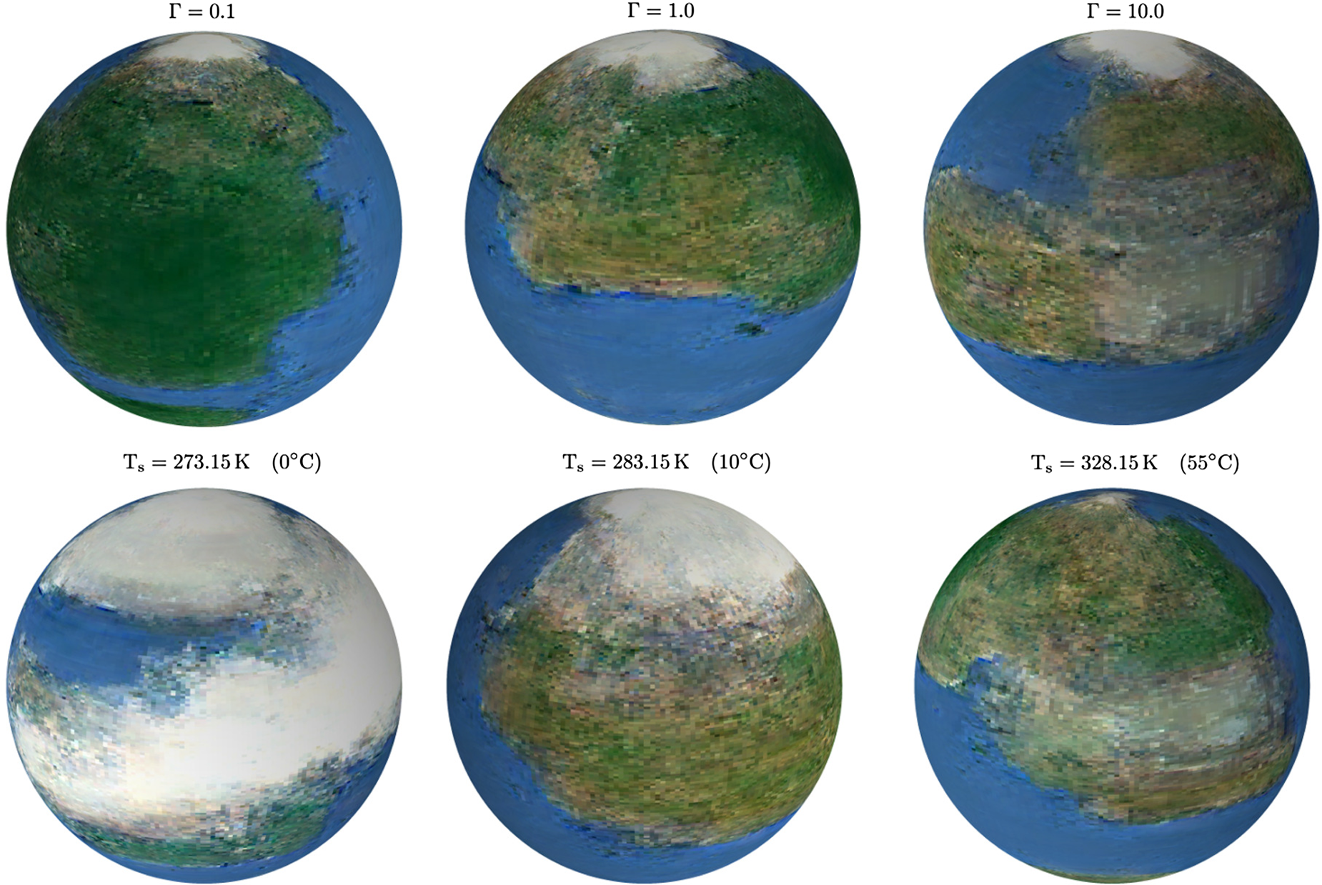
Fig. 5. Different visualizations of the Earth-Like planet for varying properties of the degassing factor, Γ (top row with land fraction γ = 0.3 and T _s = 288 K (15°C)), and global surface temperature (bottom row with γ = 0.3 and Γ = 1).

The visual appeal of the planet image generator made it a desirable addition to the website as well as the twitter bot. The main issue with the implementation was that image generation was slow, taking up to five minutes to complete; an impractical length of time for a website to load. The majority of the time was used in the rendering of the animation with the Python Matplotlib library. This was changed to use a static image of a sphere coloured according to the texture coordinates of a surface map. The image could then be modified with the surface map from the neural network for each frame of the animation, avoiding the sphere itself having to be re-rendered. This significantly reduced the time for animation production, but still produced an impractical overhead on the website if the user wanted to run multiple simulations in succession, such as in a classroom situation. This was tackled by making the creation of the visualized planet an optional addition after the website had loaded. Users can choose to run the planet image generator by pressing the ‘Render my planet’ button on a static grey globe, which then launches the neural network in the background. Once complete, the blank globe updates to the rotating planet image.

The Earth-Like interface

The Earth-Like model can be run on either the website, earthlike.world, or through the twitter bot, @earthlikeworld. Figure 6 shows the interface for the website; the classic toolkit is on the bottom-left panel, while the advanced toolkit is shown on the bottom-right. The top image in Fig. 6 shows the header on the main page of the website once the model has run. The surface temperature of the planet is displayed, along with the properties that were selected, and the present-day Earth values for comparison. On the left of the header is an animated globe, created as described in Section ‘Visualizing the planet’.

Fig. 6. The Earth-Like website interface. Bottom two panels show the top page where the planet parameters can be chosen in the classic toolkit (left) and advanced toolkit. The top panel is the header of the main page, showing the calculated surface temperature and planet image. Below the header are the model details.

Although the website speed was greatly increased by allowing the neural network to be run in the background after the page loaded, there is still a short delay due to needing run the climate model and create plots and images. Based on suggestions (see Section ‘Feedback’), we added a splash bar that shows a small animation to indicate the page is still loading. This is shown at the bottom of the lower-left panel in Fig. 6. The form submit button text also changes to read ‘simulating your planet…’ after being pressed, to emphasise that a simulation is being run. This was also in response to initial feedback that suggested users were more engaged when they knew they were running a simulation, rather than accessing a finite set of pre-calculated options.

Below the header on the main page is information on the carbon–silicate cycle and climate model that includes plots similar to those in Fig. 2 for showing the model evolution. The section on the model is subdivided into a broad overview, the model evolution which includes the plots, and a mathematical description of how the carbon–silicate box model is solved. The aim was to appeal to a broad range of readers, all of whom might wish to understand the simulation but may have differing levels of mathematical training. In the overview, a diagram of the carbon–silicate cycle is shown that is similar to Fig. 1. Arrows for the weathering and volcanism & degassing change size and colour to reflect the chosen model parameters. For example, a location near the outer edge of the habitable zone or a large land fraction would result in a wide blue coloured arrow for the weathering flux, to indicate this would have a cooling influence on the planet.

The twitter bot tweets a planet with randomly generated parameters several times a day. The tweet gives the values selected for the parameters for land fraction (γ), volcanism (degassing rate, Γ) and habitable zone position (HZ) and includes an animated image of the planet globe created as in Section ‘Visualizing the planet’. Twitter users can also control the climate model themselves by tweeting at the bot with parameters for the land fraction, volcanism and habitable zone position. The bot searches for terms ‘land’, ‘volcan’ and ‘habitable’ and numerical values, associating values with parameters based on the order they appear in the text. For the land fraction and habitable zone position, the bot allows either a fraction or a percentage to be entered. Therefore, if you wanted to run the Earth-Like model for a planet with land fraction γ = 0.7, degassing rate Γ = 9.8 and habitable zone location 0.8, any of the following would be understood:

• • A land fraction of 0.7, volcanism rate of 9.8 and habitable zone location of 0.8.

• • land fraction, volcanism, habitable zone of 0.7, 9.8, 0.8.

• • 70% land, volcano 9.8 and habitable position 80%.

An example of a tweet and the reply is shown in Fig. 7. If not all the parameters are specified, or the values chosen are out of range, then the bot selects a value at random for the missing parameter. If no parameters are specified (e.g. the tweet is ‘give me a planet!’) then the bot randomizes all parameters and challenges the user to guess the values selected based on the image of the planet. All tweets provide a link to the main page of the website, which will load the same parameter values. The advanced tool kit cannot be run from the twitter bot.

Fig. 7. The @EarthLikeWorld interface on twitter. Parameters for land fraction (γ), volcanism (degassing factor, Γ) and habitable zone position (HZ) are read by the twitter bot, which returns the Earth-like planet surface temperature, animated image and link to the main page of the website.

Since the twitter bot cannot contain information about the model, there was concern that the Earth-like planet images would suggest that all small planets are similar to our own; a message opposite to what the project wishes to portray. There is therefore a one-in-twenty chance that the twitter bot will return a simple grey image and note that current knowledge about exoplanets is limited to size, so we have no way of knowing if these worlds are truly Earth-like. This tweet is shown in Fig. 8.

Fig. 8. There is a 1 in 20 chance of tweets from @EarthLikeWorld returning a blank planet, reminding followers that our information about exoplanets is currently very limited. This occurs only when the twitter bot tweets independently, not in reply to a user tweet.

Feedback

To gain preliminary feedback on the effectiveness of Earth-Like in communicating information about planetary diversity, a questionnaire was attached to the website. Seventy-two responses were received, including a class of US high school students and a US post-graduate class for in-service physics teachers. For both these classes, no extra information about the topic was provided apart from directing students to explore the website. The demographics for all participants is shown in Fig. 9. About two-thirds of the participants can be considered not to have had scientific training beyond school. Just over half (53%) also identified themselves as being an educator. The questionnaire posed four questions about the site and an opportunity to comment further at the end of the survey. The questions posed were:

1. (i) Which statement best describes your impression of Earth-Like? (5 possible answers)

2. (ii) How did you find the information on the website? (4 possible answers)

3. (iii) What did you think of the twitter-bot? (4 possible answers)

4. (iv) You read in the media that ‘Earth 2.0’ has been discovered: an Earth-sized planet orbiting another star in the habitable zone. What is the best description of this new world? (6 possible answers)

Fig. 9. Background of the participants who completed a short questionnaire on Earth-Like from the website.

The first question targeted the overall message of the website, asking participants whether they felt the site had been informative by allowing one or more of five statements to be selected. These statements and the responses divided by demographic are shown in Fig. 10. The first three statements were consistent with the project goals, suggesting the site was a good demonstration of possible planet diversity, the evolution of the Earth and/or the factors that might affect a planet's climate. The last two statements deemed the site either uninformative or confusing. The majority of participants selected within the first three statements, suggesting the project is successful at transmitting information about planetary diversity. Just three people labelled the site confusing, although notably high school students struggled to understand the main message of the site, with six students saying the site was fun to use but not particularly informative.

Fig. 10. Responses to question 1: ‘Which statement best describes your impression of Earth-Like’ on the website questionnaire, divided by demographic.

Question 2 concerned the information available on the website, asking participants to select one of four possible statements that judged the available content to be too much or too little (Fig. 11). The majority of participants were happy with the level of detail, either finding the site sufficient or able to easily find the parts that focused their interest. A significant (24%) of participants wanted more detailed information, which this paper will provide. This request is unsurprising for scientists who might potentially wish to use the site themselves for educational or outreach activities, but interestingly both the non-scientist and student groups showed a strong interest in having access to further information. Three participants from the non-scientist and student groups did find the site contained too much information that they could not easily filter.

Fig. 11. Responses to question 2: ‘How did you find the information on the website?’ on the website questionnaire, divided by demographic.

The third question shown in Fig. 12 asked about the twitter bot. Since the questionnaire was on the website, not all participants had used the twitter bot. Of the responses from people who had explored both the website and twitter bot, the twitter bot was predominately thought a good way to play with the model and was particularly popular among the category of professionals in planet formation disciplines. This could reflect that twitter is widely used in the scientific community for sharing information (Ebner and Reinhardt Reference Ebner and Reinhardt2009; Holmberg and Thelwall Reference Holmberg and Thelwall2014).

Fig. 12. Responses to question 3: ‘What did you think of the twitter-bot?’ on the website questionnaire, divided by demographic.

The final question posed a test of the information learned on the Earth-Like site. Media articles have frequently announced the discovery of an Earth-sized exoplanet that orbits in the habitable zone using terms such as Earth 2.0. Participants were asked which statement most accurately describes what is currently known about that planet. The statements and responses by demographic are shown in Fig. 13. The correct response was statement #1: at present, we only know the radius or minimum mass of Earth-sized planets but nothing about their surface conditions. Therefore, all we can say for sure is that these planets have the same size as Earth but may not necessarily share any other similarities. Unsurprisingly, the majority of scientists selected the correct statement, as did participants in the non-scientist category. High school students did the poorest here, with the majority responding that the planet would be similar to the Earth and still likely to be habitable. This mistake may be due to assuming that the parameters presented by Earth-Like represented all possible variables in planet diversity, as opposed to the demonstration of what a small subset of possible changes could produce.

Fig. 13. Responses to question 4: ‘You read in the media that 'Earth 2.0’ has been discovered: an Earth-sized planet orbiting another star in the habitable zone. What is the best description of this new world?' on the website questionnaire, divided by demographic.