


Introduction
The Fermi Paradox highlights the disconnect between the lack of evidence for extraterrestrial intelligences (ETIs) and, using various forms of the Drake equation (see, e.g. Drake, Reference Drake2014; Olson, Reference Olson2016; Sandberg et al., Reference Sandberg, Armstrong and Cirkovic2017; Ward and Brownlee, Reference Ward and Brownlee2020), their purported high probability of existence. This prompted Enrico Fermi to ask, ‘If the Universe is teeming with aliens, then where is everybody?’ In part, this disconnect arises because it is difficult to estimate values for Drake equation variables and thus generate tractable calculations.
We approach the Fermi Paradox from a tack opposite to that of the Drake equation. Rather than calculate how many ETIs there might be, we estimate their likely catastrophic loss rate. We may not know how many alien species exist in the Milky Way, but we can generate useful estimates of how likely it is that such species, if they existed, might be debilitated before achieving advanced technological status. In particular, we identify and calculate seven ways in which astrophysical catastrophes (such as supernovae) might play such a role.
This paper is organized as follows: the first section, Introduction, describes the Drake equation and introduces a ‘catastrophe typology’, which includes the seven types of astrophysical catastrophe considered herein. The second section, Methodology, lays out key operating assumptions; describes our simple analytical model relying on a discrete, compound Poisson process and, most importantly, provides estimates of the key characteristics, measures and frequencies relating to the astrophysical catastrophes. The third section, Results and analysis, provides numerical results for the astrophysical factors, comparing and contrasting their individual and cumulative contributions to potential ETI destruction or catastrophic debilitation. The last section, Conclusions, summarizes our key findings.
Drake equation
In 1960, Frank Drake proposed an equation as a way to initiate dialogue at the first meeting on the search for extraterrestrial intelligence (Drake, Reference Drake2014). Now known as the Drake equation, it estimates the number of active, intelligent lifeforms in the Milky Way, as follows:

Here, R is the average rate of star formation; fp is the fraction of stars with habitable plants; ne is the average number of planets that can support life; fl is the fraction of planets where life develops; fi is the fraction of living species that develop intelligence; fc is the fraction of intelligent species with communications technology and L is the time civilizations will devote to interstellar communications (Webb, Reference Webb2015).
There are two drawbacks to the Drake equation. First, as originally formulated, it did not estimate the existence of ETIs as a function of time. Second, there is considerable debate about how to quantify each of the variables in equation (1) (see, e.g. Webb, Reference Webb2015). As a result, the equation has been used to justify a wide spectrum of estimates, depending on different assumptions used for each variable, with the literature ranging from one technologically advanced species in the observable Universe (us!) to millions within the Milky Way alone (Forgan, Reference Forgan2019).
Catastrophe typology
In Table 1, we set out a ‘catastrophe typology’, which summarizes various ways in which species may be prevented from reaching or maintaining advanced technological status. Component A C represents possible contributions to species debilitation caused by astrophysical catastrophes; G C, contributions to species debilitation caused by geophysical catastrophes (e.g. super volcanism); B C, contributions to species debilitation caused by biological catastrophes (e.g. species die-off via disease pandemic) and T C, contributions to species debilitation caused by socio-technological catastrophes (e.g. species die-off by nuclear war/winter).
Table 1. Catastrophe typology
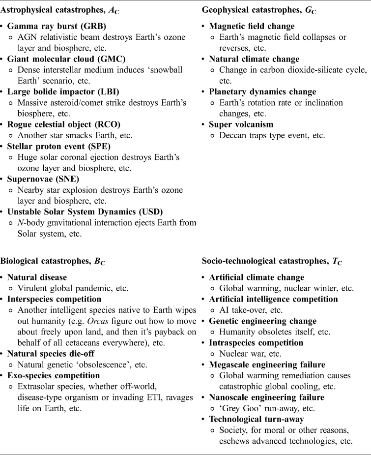
We define ‘debilitation’ as both species extinction episodes and ETI civilization-destroying events. A civilization-destroying event, while not driving an ETI species extinct, would nonetheless deprive it of advanced technological capabilities. Neither cockroaches nor cave dwellers can construct radio telescopes or build spaceships. Species extinction is thus a sufficient, but not necessary, condition for ETI debilitation.
The catastrophe typology is intended to be a comprehensive list (albeit generic), collated from the mainstream literature, in particular, Bostrom and Cirkovic (Reference Bostrom and Cirkovic2008) and Forgan (Reference Forgan2019). The catastrophic events listed in Table 1 are not mutually exclusive. Many of the catastrophes listed could interact together to form a chain of destructive events (or create self-reinforcing negative feedback loops). For example, an astrophysical catastrophe such as a large bolide strike could induce a geophysical catastrophe such as super volcanism. For the rest of this paper, we focus on astrophysical contributions, A C.
Astrophysical catastrophes: what's not included and why
Although Table 1 is intended to be comprehensive, readers familiar with the literature will note, in particular, that two astrophysical factors often implicated in species extinction – galactic winds and stellar evolution – are excluded from the A C component list. We exclude galactic winds, whose primary lethality mode is ionizing radiation (e.g. cosmic rays and secondary atmospheric muons), for two reasons. First, in our opinion, the data on the biological effects of galactic winds are not settled, e.g. Atri and Melott (Reference Atri and Melott2011) argue for the importance of galactic winds, while Bailor-Jones (Reference Bailor-Jones2009) argues against. Second, and more importantly, we already include three astrophysical sources of ionizing radiation, i.e. gamma ray bursts (GRBs), stellar proton events (SPEs) and supernovae (SNEs). The concern with including galactic winds is one of double-counting – and thus over-estimating – the source and effects of astrophysical ionizing radiation. Throughout this paper, we seek to err on the side of caution and to avoid inflated estimates for catastrophic outcomes.
The situation with respect to local stellar evolution (LSE) is quite different. All agree that stars evolve over time, entering and then departing the main sequence in which hydrogen is fused into helium. This evolutionary process significantly affects the biospheres of their planetary cohorts. Stellar evolution is dependent, to first order, on mass. The more massive the star, the faster it transitions through the main sequence, generating increased luminosity and insolation as it does so. The primary lethal effect of LSE is destruction of planetary biospheres via luminosity and insolation. Regardless of stellar mass, this is a gradual process, but the end result is always the same: planetary biospheres are destroyed. This occurs in two ways. First, planets receive so much insolation that liquid water is boiled off and, eventually, atmospheres are burned away. Second, in the case of low-to-medium mass stars (i.e. ≈1–8 solar mass), the star enters a red giant phase in which it literally engulfs its nearby planets and more-or-less burns up the rest. Clearly, then, LSE effects, in the end phase, are catastrophic. The receiving planetary system would be destroyed. However, there is nothing random or episodic about stellar evolution. LSE is not a Poisson-type catastrophic process. Species extinction and planetary destruction occur as the inevitable and predictable end-product of stellar evolution. Therefore, we conclude that it is inappropriate to assign a Poisson frequency, λ, to this type of astrophysical event. Furthermore, we assess that LSE is not a key contributor to ETI destruction. The destructive end-result of stellar evolution occurs, in most cases, long after the potential establishment of planetary biosphere. On the one hand, any ETI civilization that is technologically capable of riding out biosphere destruction via LSE should also be technologically capable of interstellar communication or spacefaring. On the other hand, any ETI civilization that is incapable of responding to the challenges posed by stellar evolution will be destroyed, but – significantly – only at the end of the nominal biosphere life cycle of its home planet. In the case of Earth, this will be approximately 5 Gyr after initiation of the planetary biosphere – more than enough time for any competent, technological species to get its act together and deal with the challenge by investing in interstellar spacefaring, and long-after the biosphere has reached its life-sustaining prime.
Remark on relation between Drake equation variable, L and our analysis
Equation (1) seeks to estimate the number of ETI civilizations that could be attempting to communicate across interstellar space. Variable L in the Drake equation estimates the timeframe in which such ETI communication attempts will occur (see, e.g. Williams, Reference Williams2020). Our analysis seeks to estimate the loss rate of ETI civilizations, however many there may be, due to astrophysical catastrophes, T C. An alternative view of our analysis is that our loss rate estimate places a hard, exogenous cap on L, i.e. L ≤ T C.
Methodology
In this section, we state our key operating assumptions (‘Key assumptions’); describe a simple analytical model relying on a discrete, compound Poisson process (‘Discrete compound Poisson process’) and analyse each of the astrophysical catastrophes comprising component A C, in terms of key characteristics, measures and frequencies (‘Astrophysical catastrophes’).
Key assumptions
We have no data on species other than those on this planet, all of which share related biochemical, genetic and environmental patterns. Theoretically, it is possible to postulate many different types of lifeforms, based on different chemical bases and reproductive patterns, inhabiting radically dissimilar environments, etc. To generate tractable calculations, we simplify along standard analytical lines, as set forth below.
Life as we know it
We restrict our analysis to carbon-based lifeforms evolving in habitable zones (HZs) in which liquid phase H2O is available.
One galaxy at a time
We restrict our analysis to the Milky Way, our barred spiral Galaxy, with stellar population between 100 and 400 billion and radius ~28.5 kpc. In what follows, unless otherwise noted, our calculations apply to the Galaxy as a whole.
Debilitation is good enough
Like Forgan (Reference Forgan2019), we broaden our analysis to include catastrophic phenomena that are capable of destroying an ETI civilization, rather than annihilating an entire species via extinction. For our purposes, species extinction is a sufficient, but not a necessary, condition.
Discrete compound Poisson process
The Poisson distribution expresses the probability of a given number of discrete events occurring in a fixed interval of time or space, if such events occur with a known constant mean rate, λ, and independently of each other. Examples of Poisson-type events include: the average number of asteroids greater than 1 km in diameter that impact Earth within an interval of 100 million years; the mean number of patients arriving in an emergency room within an interval between 10 PM and 11 PM; and the average number of cumulative failure modes for a computer within a 6-month interval.
The discrete Poisson equation is expressed in equation (2):

where P(x) is the probability of that x incidents will occur within a specified time interval. Lambda, λ, is the mean number of incidents within the specified interval. In our case, the term ‘incident’ means an astrophysical catastrophe that debilitates an ETI species, as defined above.
To find the probability, P C, that at least one astrophysical catastrophe will occur with the specified time interval, we rely on equation (3):

To calculate the cumulative effect of the astrophysical catastrophe factors, we rely on a compound Poisson process. We model potential ETIs as a complex system with multiple independent astrophysical failure modes (e.g. like an electronic circuit with multiple, independent failure points). We normalize to mean catastrophe frequencies, λ, expressed as incidents within Gyr interval. To find the cumulative effect, we compound the various normalized λ frequencies (e.g. λc = λ1 + λ2 + ⋯).
Astrophysical catastrophes
We focus on astrophysical catastrophes, A C, set forth in the catastrophe typology (Table 1). There is an extensive literature on ways in which astronomical events might, individually, destroy or catastrophically debilitate ETIs and thus contribute to resolving the Fermi Paradox (see, e.g. Hart, Reference Hart1979; Annis, Reference Annis1999; Webb, Reference Webb2015; Forgan, Reference Forgan2019). Our goal is two-fold: (a) to compare and contrast the relative importance of these contributions; and (b) to numerically assess their combined, cumulative effect as a function of time.
We do so in two different ways. First, following the standard approach in the literature, we analyse the astrophysical catastrophes in terms of their ability to cause massive, planet-wide extinction episodes, thereby annihilating a species before it could reach or maintain advanced technological status. Second, we also analyse the astrophysical catastrophes in terms of their ability to destroy an ETI civilization. We reiterate that the term ‘debilitate’ encompasses both species extinction episodes and ETI civilization-destroying events.
The key to our methodology is to identify the particular lethality modes for each astrophysical catastrophe; determine a standard – or measure – for each lethality mode and then, based on that specified measure, estimate a coarse-grained Poisson frequency, λ, of occurrence as a function of time. Unless otherwise specified, data are drawn from the existing literature.
Per Subsection ‘Discrete compound Poisson process’, our approach requires that astrophysical catastrophes occur independently of one another. To enforce this requirement, we narrowly define the lethality modes for certain astrophysical catastrophes. For example, rogue celestial objects (RCOs) are suspected to play a key role in generating large bolide impactors (LBIs) (see, e.g. Arbab and Rahvar, Reference Arbab and Rahva2021). To avoid potential double-counting, we therefore restrict the lethality mode for RCOs to disruptive ‘encounters’ (see Subsection ‘Rogue celestial objects’ for more details), on the assumption that whatever role RCOs may play in generating LBIs is already accounted for under LBI measure and frequency (see Subsection ‘Large bolide impactors’).
Another way in which we seek to avoid double-counting is by clearly defining the relationship between species extinction episodes and ETI-civilization destruction events. For our purposes, we define ETI-civilization destruction events to include species extinction episodes.
Finally, for clarity, we stress that our coarse-grained Poisson frequency estimate, for each type of astrophysical catastrophe, is intended to represent the likelihood, per unit time interval, that any random solar system within the Milky Way Galaxy would be affected by that type of astrophysical event. For example, in Subsection ‘Supernovae’, we estimate a Poisson frequency extinction rate, for SNEs, of λe = 1 Gyr−1. This does not mean that we estimate that there is only one SNE event within the Milky Way per Gyr! Rather, we are saying that any random solar system, within the Milky Way, is likely to suffer a massive species extinction event – caused by SNEs – about once during any given 1-billion-year internal.
Gamma ray bursts
Background. GRBs are highly energetic (overall energies up to 1 TeV), short-term events (milliseconds to hours), producing gamma rays and X-rays in the KeV range and cosmic rays (muons, protons, alpha particles and heavier atomic nuclei) in the MeV range. The source of GRBs is still not completely understood, but is suspected to originate from several different astrophysical phenomena, including active galactic nuclei (AGNs), which are powered by supermassive black holes residing at the centre of galaxies (ours is Sagittarius A*, mass ~4.1 million Suns, currently quiescent); neutron star mergers; black hole mergers; neutron star-black hole mergers and certain types of SNE. To date, all observed GRBs have originated outside the Milky Way (at distances ~Mpc), which is amazing given their energy and luminosity. Significantly, such energetic transfers are accomplished by beaming via relativistic jets. This beaming effect is what distinguishes GRBs from other astrophysical phenomena that also produce highly energetic ionizing radiation. Our primary references for GRBs (and SNEs and SPEs) are the review papers by Melott and Thomas (Reference Melott and Thomas2011) and Wilman et al. (Reference Wilman, Dayal, Ward, Wilman and Newman2018).
Lethality modalities. The lethality of GRBs stems from the effects of highly intense ionizing radiation. In the literature, the standard proxy for lethality is long-term (i.e. t ≥ years) depletion of planetary atmospheric ozone (O3). Ozone is important for the biosphere because it screens out destructive ultraviolet B (UVB) radiation radiating from the target planet's home star. GRB ionizing radiation dissociates ozone into oxygen (O2) via different catalytic pathways, including those involving nitrogen compounds NO and NO2 and those involving various halons. Long-term depletion of atmospheric ozone layer substantially increases biologically destructive UVB radiation levels, at the planetary surface, originating from the target planet's star (i.e. to be clear, UVB and GRBs, in this scenario, are separately sourced). The primary end result is an increase of lifeform mortality and damage, on the target planet's surface, via DNA destruction and mutation as well as disruption of key biochemical pathways, thereby causing skin cancers, cataracts, sunburn, etc.
Species extinction versus civilization destruction measures. Following both Melott and Thomas (Reference Melott and Thomas2011) and Wilman et al. (Reference Wilman, Dayal, Ward, Wilman and Newman2018), for the scenario of planetary-wide species extinction episodes caused by GRBs, we set the measure to an atmospheric fluence of 100 kJ m−2 (based on gamma rays in the 200 KeV range). This corresponds to 30% depletion of average planetary atmospheric ozone layer. For ETI civilization-destroying events, we set the measure to an atmospheric fluence of 32 kJ m−2 (or about 1/3 the extinction level, based on gamma rays in the 200 KeV range).
Species extinction (λe) versus civilization destruction (λd) Poisson frequencies. Not surprisingly, given the unknowns and complexities surrounding GRB processes and lethality (e.g. see Subsection ‘Remarks on astrophysical ionizing radiation’ below), experts differ on the rate at which GRBs contribute to species extinction within our Galaxy. Melott and Thomas (Reference Melott and Thomas2011) estimate λe = 4 Gyr−1 for planet-wide species extinction episodes based on all types of GRB (i.e. both short-hard GRBs and long-soft GRBs). They express their figure as an ‘order of magnitude estimate’, which results in a range of galaxy-wide GRB-induced extinction episodes between 0.2 and 20 Gyr−1. More recently, Wilman et al. (Reference Wilman, Dayal, Ward, Wilman and Newman2018) estimate a much lower GRB extinction rate, based on nuanced estimates taking into consideration galactic time evolution (especially relating to changing stellar metallicity rates) and galactic region (distance from galactic centre). The average of their estimated ranges within the Milky Way is 0.51 ± 0.32 Gyr−1 (arithmetic mean ± 68% Confidence Level (C.L.)). However, the estimate of Wilman et al. (Reference Wilman, Dayal, Ward, Wilman and Newman2018) only includes long-duration GRBs. Significantly, neither group includes the deleterious effects of cosmic ray showers associated with GRBs. Dar (Reference Dar, Bostrom and Cirkovic2008) estimates that cosmic ray beams from galactic GRBs can reach galactic distances (~25 000 ly) and ‘can be much more lethal than their gamma-rays’. Taking the varying estimates into consideration, and seeking to err on the side of caution, we estimate the overall GRB extinction rate, for any given solar system within the Milky Way, to be λe = 0.6 Gyr−1. As for civilization-destroying rates (based on a measure of 32 kJ m−2 GRB UVB fluence), we interpolate fig. 1 in Melott and Thomas to set the interval at 2.1 per 108 years (combining rates for all types of GRBs), or 21 Gyr−1. On the other hand, Wilman et al. (Reference Wilman, Dayal, Ward, Wilman and Newman2018) estimate 10 kJ m−2 GRB UVB fluence rates to be an order of magnitude higher than their 100 kJ m−2 GRB UVB fluence estimate, which correlates with a galaxy-wide average rate of approximately λd = 3 Gyr−1 over the history of the Milky Way. Since our measure is three times higher than Wilman et al. (Reference Wilman, Dayal, Ward, Wilman and Newman2018), we estimate λd = 1.8 Gyr−1. In conclusion, based on a review of the literature, our estimated GRB rates are λe = 0.6 Gyr−1 and λd = 1.8 Gyr−1 for average galaxy-wide extinction episodes and civilization destruction events, respectively. We consider both figures to be ‘order of magnitude’ estimates.
Remarks on astrophysical ionizing radiation. We offer three remarks concerning astrophysical ionizing radiation. First, there are numerous and highly variable sources, including AGNs, neutron star mergers; black hole mergers; neutron star-black hole mergers; SNEs; stellar flares and coronal mass injections; pulsars; magnetars; galactic cosmic rays (‘galactic wind’) and secondary effects created by LBIs. Just how these sources are categorized is somewhat arbitrary. For our analysis, we group astrophysical ionizing radiation into three broad categories, based on physical mechanism and distance between source and planetary target: GRBs (Subsection ‘Gamma ray bursts’), with fluence mechanism based on relativistic beaming occurring at intergalactic distances (~Mpc); SPEs (Subsection ‘Stellar proton events’), with fluence mechanism based on solar flares and coronal mass ejections occurring at interplanetary distances (~AU) and SNEs (Subsection ‘Supernovae’), with fluence mechanism based on stellar explosions occurring within regions of the Milky Way (with lethal distances ~pc). Second, the standard picture of lethality for astrophysical ionizing radiation is indirect. The primary proxy for lethality is long-term, large-scale depletion of planetary atmospheric ozone. Just what constitutes ‘long-term’ and ‘large-scale’ depletion are debatable. Third, reliance on atmospheric ozone as the primary lethality proxy encodes several assumptions, such as that the target planet in question has atmospheric ozone; that atmospheric ozone plays a key role in the planetary biosphere; that the planet's star produces dangerous levels of UVB and that organisms on the planet have evolved to be susceptible to that UVB radiation. Thus, while experts agree that such radiation can – potentially – catastrophically affect planetary biospheres, the causal chain for astrophysical ionizing radiation debilitation is both complex and uncertain.
Giant molecular clouds
Background. Solar systems encounter varying densities of interstellar medium (‘dust’). This dust consists primarily of hydrogen atoms with other associated baryonic gaseous debris. The density of our local interstellar medium is currently ~0.2 H cm−3. When density of the interstellar medium exceeds 100–300 H cm−3, it is often referred to as a ‘giant molecular cloud’ (GMC). GMCs can be large and massive, extending across 100 pc and comprising up to several million solar masses. As the Milky Way rotates, solar systems – including ours – are swept through GMCs, especially in the spiral arms. Our primary reference for GMCs is Pavlov et al. (Reference Pavlov, Toon, Pavlov, Bally and Pollard2005).
Lethality modalities. GMCs are linked to planetary biosphere damage and species debilitation in several different ways, including long-term global ozone depletion via increased galactic cosmic ray flux; initiation of nearby SNEs and ensuing intense ionizing radiation and associated long-term global ozone depletion; enhanced creation of LBIs via gravitational tidal disruption of the Oort-type clouds and enhanced planetary glaciation via reduction of solar insolation.
For reasons discussed in Subsection ‘Remarks’ below, we specify the primary lethality mode of GMCs as enhanced glaciation. The lethality mechanism works as follows, as exemplified by our Solar System. Plasma ejected by the Sun creates a heliosphere, or a ‘safe space’ (bubble) that surrounds the Solar System, including Earth. Within this bubble, planets are partially protected from ionized particles infalling from the interstellar medium, SNEs, etc. However, GMCs of sufficient size and density are capable of reducing or even collapsing the heliosphere. Once the heliosphere collapses, interstellar dust particles can accrete directly into the Earth's atmosphere. These particles then absorb and scatter the Sun's insolation in the visible frequencies (but not infrared frequencies!). The end result is an ‘anti-greenhouse effect’, which leads to cooling of planetary surface and lower atmosphere. If the cooling effect is sufficiently robust, the entire planet can be subjected to runaway glaciation: the ‘snowball Earth’ scenario.
Species extinction versus civilization destruction measures. For the scenario of planetary-wide species extinction episodes caused by GMCs (i.e. snowball Earth scenario), we set the measure equivalent to an encounter with a cloud of ~5000 H cm−3, which would imply a radiative forcing of approximately −15 W m−2, for ≳100 000 years. For ETI civilization-destroying GMCs, we set the measure equivalent to a collision with a cloud of ~2000 H cm−3, which would imply a radiative forcing of approximately −10 W m−2, for ≳100 000 years. This radiative negative forcing would induce a mini-Ice Age worse than the Quaternary Glaciation. For comparative purposes, the Mt. Pinatubo eruption, of 15 June 1991, produced a radiative negative forcing of ~2–4 W m−2, causing global cooling of 0.5°C for a year.
Species extinction (λe) versus civilization destruction (λd) Poisson frequencies. Relying on Pavlov et al. (Reference Pavlov, Toon, Pavlov, Bally and Pollard2005), we set the GMC snowball Earth mass extinction frequency λe = 1 Gyr−1. We set the interval (frequency) for civilization-destroying GMCs to be approximately 5 × 10⁸ years, or λd = 2 Gyr−1. Both figures are ‘order of magnitude’ estimates.
Remarks. We restrict GMC lethality to enhanced glaciation scenarios. We do so to avoid the possibility of ‘double counting’. As noted in Subsection ‘Background’, GMCs have also been implicated catastrophes involving ozone depletion via galactic cosmic rays and SNEs ionizing radiation as well as via enhanced LBI creation. We do not consider these additional lethality modes here, as they are already addressed in Subsections ‘Gamma ray bursts’, ‘Stellar proton events’ and ‘Supernovae’ as well as in Subsection ‘Large bolide impactors’, respectively.
Large bolide impactors
Background. LBIs include both asteroids and comets, whose planetary impact is typically accompanied by a large atmospheric fireball. On the one hand, we have no data on how LBIs affect other solar systems throughout the Milky Way, much less those hosting hypothesized ETIs. On the other hand, we have excellent data on LBI effects on Earth, which have remained relatively constant – in type and frequency – over the last ~3.5 Gyr. Furthermore, we have no reason to suppose that our Solar System is atypical with respect to LBIs, except to note that the Earth–Moon system may be more robust in ameliorating LBI effects than planets without a large moon (see Subsection ‘Remarks on estimating LBI frequency’ below). Our primary reference for LBIs is Chapman (Reference Chapman2004).
Lethality modalities. On Earth, LBIs are well-known for triggering major extinction episodes. For example, the KT extinction event, which wiped out ~75% of land and sea species about 66 Mya, was likely caused by a bolide (asteroid or comet, exact type unknown) impactor approximately 10–15 km in diameter. LBI primary effects are: massive and sudden injection of thermal energy into the planetary system; prompt, large-scale blast and shockwaves, originating from an atmospheric fireball, which propagate throughout the planetary atmosphere and large-scale destructive impact on planetary surface. Key secondary effects include: fragmentation debris bombardment across much of planetary surface; massive conflagrations on land; large-scale injection of soot and other particulate matter into atmosphere, causing major reduction in solar flux, thereby leading to regional or global cooling, from months to decades; widespread earthquakes on land, and at sea, causing mega tsunamis and destabilization of ecosphere, such as profound changes in atmospheric and seawater chemistry, ozone layer loss or initiation of enhanced volcanism. Significantly, the cumulative effect of these actions is the widespread die off of lifeforms, most notably affected being large organisms that inhabit either food chain apexes or specialized ecological niches, which, presumably, best describe any ETI species.
Species extinction versus civilization destruction measures. For the scenario of planetary-wide species extinction episodes caused by LBIs, we set the measure equivalent to the Cretaceous-Tertiary (KT)-type impactor. Such an impactor would have diameter ≥10 km and an impact energy ≥108 megatons of TNT (trinitrotoluene) equivalent (i.e. 108 MT) energy. In this regard, 1 tonne of TNT is defined, in terms of energy release (often referred to as ‘explosive yield’), as:

Thus, planetary-extinction LBIs would abruptly inject at least ~1023 J into the impacted planetary ecological system.
Following Chapman, for ETI civilization-destroying LBIs, we set the measure equivalent to an impactor with diameter ≥2 km and an impact energy ≥106 MT. This impactor would thus be about 1/100 size of KT-type impactor, in terms of kinetic energy release, yet still capable of destroying a continent and causing planet-wide negative climatological effects. For comparative purposes, the 6 August 1945, Hiroshima nuclear weapon attack was a 0.15 MT airburst, which resulted in approximately 40 000 ‘prompt fatalities’ (deaths within 24 h), almost all caused by thermal radiation and blast/shockwave effects (vice initial or residual nuclear radiation); the 30 June 1908, Tunguska event was a 100 m diameter bolide airburst (type unknown), yielding ~15 MT, which levelled approximately 2000 km2 of largely uninhabited Siberian forest and the 15 February 2013, Chelyabinsk event was a 20 m diameter bolide airburst (asteroid), yielding ~0.5 MT, which injured approximately 1500 individuals and damaged almost 7200 buildings.
Species extinction (λe) versus civilization destruction (λd) Poisson frequencies. Relying on fig. 1 in Chapman, we interpolate the impact interval (frequency) for KT impactors to be approximately 108.5 years = 3.16 × 10⁸ years. Normalizing to Gyr, and assuming a Poisson impact process, we set λe = 30 Gyr−1 for species extinction episodes. Similarly, we interpolate the impact interval (frequency) for civilization-destroying LBIs to be approximately 107 years, or λd = 100 Gyr−1. Both figures are ‘order of magnitude’ estimates.
Remarks on estimating LBI frequency. Chapman's analysis is restricted to asteroids; comet impactors are not included. Chapman estimates that comets would contribute an additional 1% to λ frequency. Similarly, following Ward and Brownlee (Reference Ward and Brownlee2020), we acknowledge that the Earth–Moon system is likely atypical. In effect, the Moon serves as a non-trivial shield or buffer against impactors, thus decreasing λ frequency as compared to an ‘average’ planetary system. In estimating λ frequencies for LBIs, we do not take these two factors into account and thus our λ values could be underestimates.
Rogue celestial objects
Background. RCOs include stars, black holes and planetoids that are not initially gravitationally bound to the solar system in question (i.e. they are just ‘passing through’ or are in the process of being gravitationally captured by the home system). What these objects have in common is sufficient mass to, at a minimum, substantially perturb the receiving system. Asteroids and comets are not included as RCOs, as they are treated in Subsection ‘Large bolide impactors’ as LBIs. Our primary reference for RCOs is Arbab and Rahvar (Reference Arbab and Rahva2021).
Lethality modalities. Lethality arises in terms of an ‘encounter’, which can take four forms. First, the encounter can be a direct collision. Second, the encounter can be a ‘near miss’, which perturbs the home planet's biosphere through gravitational effects, electromagnetic effects, etc. Third, the encounter can be a gravitational perturbation of the home planet's orbital parameters, culminating in ejection of the home planet from its solar system. Fourth, the encounter can be a gravitational perturbation of the home planet's orbital parameters, culminating in shifting the home planet out of its Habitable Zone (HZ), while still staying gravitationally bound to its home system.
Species extinction versus civilization destruction measures. As specified above, all such RCO encounters would be catastrophic. The biosphere of the receiving planetary system would be destroyed. Therefore, in the case of RCOs, we make no distinction between species extinction episodes and ETI civilization-destroying events.
Species extinction versus civilization destruction Poisson frequencies (λ). Arbab and Rahvar (Reference Arbab and Rahva2021) calculate λ = 0.98 × 10⁻⁴ Gyr−1 for stellar encounters near our solar neighbourhood and λ = 5.36 × 10⁻⁴ Gyr−1 for stellar encounters within the Milky Way bulge environment. We take the geometric mean of the Arbab and Rahvar (Reference Arbab and Rahva2021) estimates, and rounding down, set λ = 2.0 × 10⁻⁴ Gyr−1 as the frequency for both species extinction episodes and ETI civilization-destroying events involving RCOs. This figure is an ‘order of magnitude’ estimate.
Remarks on estimating RCO frequency. Arbab and Rahvar (Reference Arbab and Rahva2021) conclude that stellar encounters ‘are very rare’, which tracks with other analyses in the literature (see, e.g. Forgan, Reference Forgan2019). However, we note that Arbab and Rahvar (Reference Arbab and Rahva2021) only analyse stellar encounters; they do not address rogue black holes or planetoids. Therefore, the RCO frequency of λ = 2 × 10⁻⁴ Gyr−1 could be an underestimate.
Stellar proton events
Background. Local SPEs encompass multiple highly energetic explosions from the Sun, including solar flares and coronal mass ejections. Solar flares are flashes of intense light radiation, occurring at various wavelengths, which erupt from a small section on the Sun. Coronal mass ejections are giant clouds of particles, plasma and magnetic fields that are ejected from the Sun. Solar flares and coronal mass ejections are often associated with one another but can occur independently. Our primary references for SPEs are Melott and Thomas (Reference Melott and Thomas2011), Rohen et al. (Reference Rohen, von Savigny, Sinnhuber, Llewellyn, Kaiser, Jackman, Kallenrode, Schroter, Eichmann and Bovensmann2005) and Wilman et al. (Reference Wilman, Dayal, Ward, Wilman and Newman2018).
Lethality modalities. The lethality of SPEs stem from their highly intense ionizing radiation. In the literature, the standard proxy for lethality is long-term (i.e. t ≥ ~years) depletion of planetary atmospheric ozone (O3). Ozone is important for the biosphere because it screens out destructive UVB radiation radiating from the target planet's home star. Solar flares and coronal mass ejections release protons that break up molecules of atmospheric gases such, as nitrogen (N2) and water vapour, which react with and reduce ozone. During a SPE event the incident highly energetic protons ionize the major atmospheric molecules N2 + (58.5% partitioning of total ionization), N + (18.5%), O + (15.4%) and O2 + (7.6%). Long-term depletion of atmospheric ozone layer substantially increases biologically destructive UVB radiation levels, at the planetary surface, originating from the target planet's star (i.e. to be clear, UVB and SNEs, in this scenario, are separately sourced). The primary end result is an increase of lifeform mortality and damage, on the target planet's surface, via DNA destruction and mutation as well as disruption of chemical bonds in key biochemical pathways, thereby causing skin cancers, cataracts, sunburn, etc.
Species extinction versus civilization destruction measures. Following both Melott and Thomas (Reference Melott and Thomas2011) and Wilman et al. (Reference Wilman, Dayal, Ward, Wilman and Newman2018), for the scenario of planetary-wide species extinction episodes caused by SPEs, we set the measure to an atmospheric fluence of 100 kJ m−2. This corresponds to 30% depletion of average planetary atmospheric ozone layer. For ETI civilization-destroying events, we set the measure to an atmospheric fluence of 32 kJ m−2 (or about 1/3 the extinction level).
Species extinction (λe) versus civilization destruction (λd) Poisson frequencies. Relying on fig. 1 in Melott and Thomas (Reference Melott and Thomas2011), we linearly extrapolate the SPE curve to set λe = 0.1 Gyr−1 for planet-wide species extinction episodes based on SPEs. Based on a civilization-destroying measure of 32 kJ m−2 UVB fluence, we linearly extrapolate SPE curve in fig. 1 in Melott and Thomas to set the interval at 1 per 109 years, or λd = 1 Gyr−1. Both figures are ‘order of magnitude’ estimates.
Remarks. See Subsection ‘Gamma ray bursts’, for general remarks concerning astrophysical ionizing radiation.
Supernovae
Background. SNEs are catastrophic explosions of certain types of star at the end of their evolutionary cycle. Although there are various kinds of SNEs, such as type Ia (thermal runaway) and type IIP (core collapse), the physics of SNEs is relatively well-known (see, e.g. Carroll and Ostlie, Reference Carroll and Ostlie2007). Like GRBs and SPEs, the primary result of these catastrophic explosions is production of highly energetic gamma ray and X-ray photons (peak fluence ~1039 J over seconds to hours) as well as highly energetic cosmic rays (~1017 eV). Unlike GRBs, transmission of fluence does not involve relativistic beaming effects; rather, the stellar explosion produces a roughly spherical wave front, which propagates and dissipates, to first order, as distance, ~D 1/3. As a result, effects are confined to the Galaxy. Many researchers set the ‘lethal distance’ for SNEs at about 10 pc. This seems to be a relatively small fraction of the Galaxy as a whole. However, researchers estimate that 2–3 SNEs occur throughout the Milky Way every 100 years, or ~25 000 000 Gyr−1. Our primary references for SNEs are Melott and Thomas (Reference Melott and Thomas2011) and Wilman et al. (Reference Wilman, Dayal, Ward, Wilman and Newman2018).
Lethality modalities. Like GRBs and SPEs, the lethality of supernova stems from the effects of highly intense ionizing radiation. In the literature, the standard proxy for lethality is long-term (i.e. t ≥ ~years) depletion of planetary atmospheric ozone (O3). Ozone is important for the biosphere because it screens out destructive UVB radiation radiating from the target planet's home star. Ionizing radiation dissociates ozone into oxygen (O2) via different catalytic pathways, including those involving nitrogen compounds NO and NO2 and those involving various halons (e.g. Cl, Br, etc.). Long-term depletion of atmospheric ozone layer substantially increases biologically destructive UVB radiation levels, at the planetary surface, originating from the target planet's star (i.e. to be clear, UVB and SNEs, in this scenario, are separately sourced). The primary end result is an increase of lifeform mortality and damage, on the target planet's surface, via DNA destruction and mutation as well as disruption of chemical bonds in key biochemical pathways, thereby causing skin cancers, cataracts, sunburn, etc.
Species extinction versus civilization destruction measures. Following both Melott and Thomas (Reference Melott and Thomas2011) and Wilman et al. (Reference Wilman, Dayal, Ward, Wilman and Newman2018), for the scenario of planetary-wide species extinction episodes caused by SNEs, we set the measure to an atmospheric fluence of 100 kJ m−2 (based on gamma rays in the 200 KeV range, and assuming a maximum lethality range of 10 pc). This corresponds to 30% depletion of average planetary atmospheric ozone layer. For ETI civilization-destroying events, we set the measure to an atmospheric fluence of 32 kJ m−2 (or about 1/3 the extinction level, based on gamma rays in the 200 KeV range).
Species extinction (λe) versus civilization destruction (λd) Poisson frequencies. As with GRBs, experts disagree on the frequency of catastrophic SNEs within the Milky Way. On the one hand, Melott and Thomas (Reference Melott and Thomas2011) estimate λe = 2 Gyr−1 for planet-wide species extinction episodes based on SNEs (see their fig. 1), assuming a generic lethality range of ~10 pc. Based on a civilization-destroying measure of 32 kJ m−2 UVB fluence, we interpolate fig. 1 in Melott and Thomas (Reference Melott and Thomas2011) to estimate λd = 18 Gyr−1. On the other hand, Wilman et al. (Reference Wilman, Dayal, Ward, Wilman and Newman2018) estimate a lower frequency, on the order of λe = 1 Gyr−1. This estimate tracks with Dar (Reference Dar, Bostrom and Cirkovic2008). As for the frequency of civilization destroying SNEs, we estimate a frequency three times greater than that for extinction episodes, so that λd = 3 Gyr−1. In conclusion, based on a review of the literature and erring on the side of caution, we estimate SNE rates as λe = 1 Gyr−1 and λd = 3 Gyr−1 for average galaxy-wide extinction episodes and civilization destruction events, respectively. Both figures are ‘order of magnitude’ estimates.
Remarks on astrophysical ionizing radiation. See Subsection ‘Gamma ray bursts’, for general remarks concerning astrophysical ionizing radiation.
Unstable solar system dynamics (USDs)
Background. Solar systems are inherently unstable, particularly over prolonged intervals (~10 million years or more). Gravitational interactions amongst planets can perturb planetary dynamical parameters, particularly orbital eccentricity and inclination (a classic example of the N-body problem). The result is chaotic solar system motion, in which even small gravitational effects over the long-term lead to unpredictable and possibly catastrophic planetary orbital behaviour. Interactions with asteroids and comets are not included as USDs, as they are treated in Subsection ‘Large bolide impactors’ as LBIs. Similarly, gravitational perturbations involving objects originating outside the solar system are not included as USDs, as they are treated in Subsection ‘Rogue celestial objects’ as RCOs. Our primary references for USDs are Laskar and Gastineau (Reference Laskar and Gastineau2008), Laskar (Reference Laskar2013) and Laskar (Reference Laskar1994).
Lethality modalities. Lethality arises in terms of an ‘instability’, caused by chaotic gravitational perturbation, which can take four forms. First, the instability can lead to direct collision between two or more home system planets (or between planets and the home star). Second, the instability can be a ‘near miss’ between two or more home system planets (or home star), which perturbs the receiving planet's biosphere through gravitational effects, electromagnetic effects, etc. Third, the instability can cause the ejection of the planet from its home solar system. Fourth, the instability can cause the planet to shift out of its HZ, while still staying gravitationally bound to its home system.
Species extinction versus civilization destruction measures. As specified above, all such USD instabilities would be catastrophic. The biosphere of the receiving planetary system would be destroyed. Therefore, in the case of USDs, we make no distinction between species extinction episodes and ETI civilization-destroying events.
Species extinction versus civilization destruction Poisson frequencies (λ). Estimating catastrophic orbital instability frequencies is tricky. Every solar system within the Milky Way is different. As the instabilities are, by definition, the product of chaotic perturbations, prediction is difficult. Therefore, generating precise yet reliable frequency estimates – on a galaxy-wide basis – is a difficult challenge. In the case of our Solar System, the procedure is to numerically integrate planetary interactions, across a timeframe of the 5 Gyr (i.e. the lifespan of our Solar System), in which initial conditions are slightly varied over the course of hundreds or thousands of simulated evolution scenarios. In general, research groups find a small (~1%) but persistent probability that gravitational perturbations will lead to catastrophically chaotic scenarios, in which planets collide, fall into the Sun or are ejected from the Solar System, within a timeframe on the order of 100 million years to 5 billion years. Seeking to err on the side of moderation, we set λ = 0.1 Gyr−1 as the Poisson frequency for both species extinction episodes and ETI civilization-destroying events involving USDs. This figure is an ‘order of magnitude’ estimate.
Remarks on estimating USD frequency. In addition to the inherent difficulty of calculating USD frequencies, we stress that interactions involving LBIs or RCOs can have similar consequences and can create mutually reinforcing catastrophic feedback loops. For example, a massive comet or asteroid, in addition to smacking Earth directly, could also perturb the orbit of Mars, resulting in a ‘double whammy’ as Mars then negatively interacts with Earth. To avoid such potential double-counting scenarios, we have adopted a de minimis value for USD frequencies.
Table 2 summarizes the debilitation modes, measures and frequencies, for both planet-wide extinction episodes and civilization-destroying events, for each type of astrophysical existential threat discussed above.
Table 2. Summary astrophysical catastrophe types and frequencies

Results and analysis
In this section, we calculate the coarse-grained likelihood, on a galaxy-wide basis, that seven types of astrophysical catastrophe could cause massive species extinction episodes or destroy ETI civilizations. Calculations are based on equations (2) and (3) set forth in Subsection ‘Discrete compound Poisson process’. Poisson frequency values, λ, are drawn from the estimates set forth in Subsection ‘Astrophysical catastrophes’, which are summarized in Table 2. Numerical results are presented in Subsection ‘Results’; in Subsection ‘Error estimates’, we comment on error estimates for numerical results; and in Subsection ‘Discussion’ we analyse and discuss the significance of our results.
Results
We provide two sets of tables in this subsection. The first set, Tables 3–6, lists the probability of massive species extinction episodes for each type of astrophysical catastrophe, on the intervals of 1.0, 0.1, 0.01 and 0.001 Gyr. The second set, Tables 7–10, lists the probability of ETI civilization destruction events, using the same time intervals. We also combine all astrophysical catastrophe types to provide overall probabilities for both species extinction and ETI civilization destruction on the four specified time intervals. As for the choice of time intervals, we note that 1 Gyr corresponds to the estimated mean lifetime of planetary HZ due to a ‘Gaian bottleneck’ (see, e.g. Chopra and Lineweaver, Reference Chopra and Lineweaver2016); 0.1 Gyr corresponds to the estimated frequency of many of the astrophysical factors discussed above; 0.01 Gyr corresponds to the estimated mean lifespan of species on Earth (see, e.g. Mills, Reference Mills2012; Newman, Reference Newman1997) and 0.001 Gyr corresponds roughly to the current lifespan of the human species.
Table 3. Likelihood species extinction by astrophysical catastrophe (A extinction)

Table 4. Likelihood species extinction by astrophysical catastrophe (A extinction)

Table 5. Likelihood species extinction by astrophysical catastrophe (A extinction)

Table 6. Likelihood species extinction by astrophysical catastrophe (A extinction)

Table 7. Likelihood civilization destruction by astrophysical catastrophe (A destruction)

Table 8. Likelihood civilization destruction by astrophysical catastrophe (A destruction)
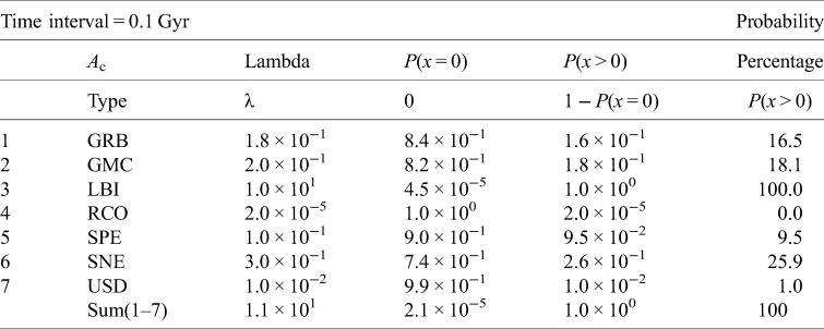
Table 9. Likelihood civilization destruction by astrophysical catastrophe (A destruction)
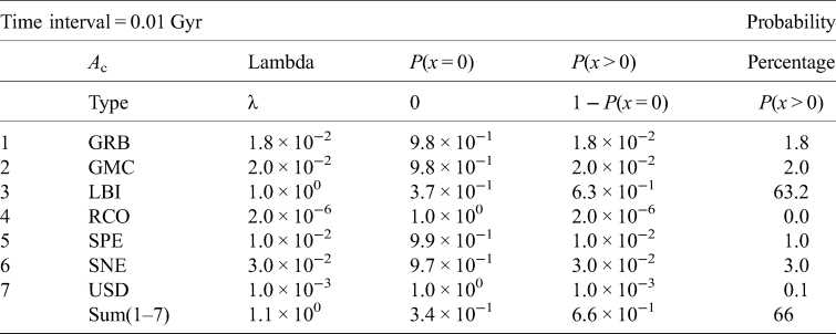
Table 10. Likelihood civilization destruction by astrophysical catastrophe (A destruction)

Error estimates
All of our estimates for frequencies, λ, are ‘order of magnitude’ estimates, as stated in Subsection ‘Astrophysical catastrophes’. Hence, the absence of error bars on specific numerical results in this section. We emphasize that the frequencies set forth in Subsection ‘Astrophysical catastrophes’, and used in this section, are estimates; they do not constitute actual measured Poisson counts. As a result, it is inappropriate to attach error bars based on $\sqrt \lambda$ , as would customarily be the case in Poisson-type analyses.
Discussion
In this subsection, we discuss and analyse results; specifically, compare the destructiveness of the seven types of astrophysical threats; analyse significance of calculated species extinction rates versus ETI civilization destruction rates; consider ways species might avoid or ameliorate astrophysical catastrophes and evaluate the likely contribution of astrophysical existential threats to resolving the Fermi Paradox.
Comparing the astrophysical existential threats. In terms of relative contributions by type of astrophysical catastrophe, the most significant player is LBIs. LBIs are more than three times as likely to occur as all other astrophysical catastrophes combined. They are also potentially highly destructive. LBIs are truly the ‘heavy hitters’ in the world of astrophysical existential threats. After LBIs, the three most likely types of astrophysical catastrophe are SNEs, GMCs, and GRBs, all with roughly the same frequency, each an order of magnitude less prevalent than LBIs. The potentially most destructive astrophysical catastrophes – RCOs and USDs – have the lowest frequencies, and appear to be relatively de minimis threats (thankfully!). Finally, our closest type of astrophysical threat – solar proton events (SPEs, such as coronal mass ejections) – also appears to relatively minor existential threats.
Species extinction. Our results indicate that there is almost a 100% probability that both massive species extinction could occur, on an interval of about every 100 million years (and, of course, on intervals of Gyr or greater), to any solar system within our Galaxy. At the 10-million-year interval, the probability that extinction will occur is roughly 28%. At the 1-million-year interval, the probability that extinction will occur is only 3%.
Focusing on the 100-million-year interval, our results indicate that any planetary system within the Milky Way is statistically likely to suffer at least one massive species die off due to an astrophysical event within any given time interval of 100 million years. On the one hand, this does not guarantee that a sentient species, even if it failed to take prophylactic action, would be driven extinct. Our results only indicate that such a species would observe or be associated with such a massive die off, which might or might not lead to its own demise, whether over the short term or long term.
On the other hand, we interpret our results to apply to all planets within the receiving solar system. In the cases of GRBs, SNEs and GMCs, the effects would likely simultaneously affect all planets in the system. Depending on their type and characteristics, the same could be for RCOs and USDs (and possibly SPEs), too. As for LBIs, their effects would be most likely limited to a particular planet within system. However, cratering observed on all of Sol's inner planets clearly indicates that LBI bombardment is an ongoing existential threat to each and every planet within our Solar System.
We interpret our 100-million-year interval result to mean that any species, within our Galaxy, has roughly 100 million years to evolve from a complex lifeform (e.g. multicellular organism) to a spacefaring civilization. We see this as a definite astrophysical ‘extinction bottleneck’, analogous to Chopra and Lineweaver's (Reference Chopra and Lineweaver2016) ‘Gaian bottleneck’.
Our 10-million-year interval result of 28% is, in one sense, shocking. This result implies the possibility that any species, within our Galaxy and over the course of its history, stands something like a 1-in-4 chance of seeing in a massive species die off caused by an astrophysical catastrophe. To put that result into perspective, here on Earth, the average longevity for species is on the order of 10 million years, per Mills (Reference Mills2012) and Newman (Reference Newman1997). On the bright side, this implies that astrophysical effects cannot be the primary cause of ‘typical’, ongoing species extinction.
The 1-million-year interval extinction rate of 3% is heartening. Apparently, if the human race is to go extinct within the next 1 million years, it likely will not be due to an astrophysical catastrophe!
Civilization destruction. Our results indicate that there is a 100% probability that ETI civilization destruction could occur, on an interval of about every 100 million years, to any solar system within our Galaxy due to astrophysical catastrophes. At the 10-million-year interval, the probability that ETI civilization destruction will occur is about 66%! At the 1-million-year interval, the probability that ETI civilization destruction will occur is roughly about 10%.
We acknowledge that the significance of results presented in Tables 7–10 is problematical and thus debatable. We have never observed an ETI-civilization, much less one that was destroyed by, or rebounded back from, an astrophysical catastrophe. Therefore, we cannot make tractable estimates about how such a civilization might fare or respond in a lower type of astrophysical disaster, which might badly damage part or all of a planet's biosphere yet not cause massive species die off. We include the category of ‘civilization destruction’ to highlight the possibility that sentient species – and even spacefaring civilizations – might be derailed by astrophysical effects that do not rise to the level of planetary obliteration. This line of analysis requires much more effort.
Responses to astrophysical existential threats. Our calculations do not consider the possibility that sentient species, particularly spacefaring species, might be able to engage in prophylactic action in the face of astrophysical existential threats. Possible prophylactic action could include ‘hardening’ the receiving system against deleterious astrophysical effects or fleeing the planetary system before it is astrophysically debilitated. There is both good news and bad news.
The bad news is that some types of astrophysical catastrophe are almost impossible to protect against. In the face of an RCO or an USD, the only hope would seem to be to flee the receiving system before disaster, assuming there was sufficient warning (which would depend on the type of disaster and the technological sophistication and resoluteness of the species under threat). Other astrophysical threats, such as GRBs, SNEs, SPEs and GMCs, could be proactively hardened against, but such prophylactic action could require massive diversion of resources, perhaps amounting to planetary-level geoengineering projects. Technically, such actions are possible; whether the species in question would have the opportunity, resources and wisdom to undertake them is another matter.
The good news concerns LBIs. Our analysis indicates that they are, by far, the most prevalent type of astrophysical catastrophe and potentially one of the most destructive. Significantly, asteroid and cometary impacts also are, with reasonable investment in resources, both the most predictable and the most preventable of all astrophysical existential threats. Thus, the direct threat posed by LBIs boils down, primarily, to a combination of environmental timing and species behaviour. For example, on Earth, the dinosaurs had the bad luck to be wiped out by a bolide impactor before reaching advanced technological status. Our species has achieved that milestone. The only thing stopping us now from prophylactic action in the face of LBI existential threats is our own behaviour – and, of course, the other existential threats listed in Table 1. (In this regard, one is reminded of the 2021 movie Don't Look Up.)
Astrophysical existential threats and the Fermi Paradox. We conclude our analysis by addressing the possible relevance of astrophysical catastrophes to resolving the Fermi Paradox. Can the seven astrophysical existential threats analysed herein – whether singly or in combination – explain why we do not see any evidence of ETIs within the Milky Way? Our analysis indicates that astrophysical catastrophes pose a significant existential threat to species throughout our Galaxy, in the past, at present and into the foreseeable future. Nonetheless, our conclusion is a ‘nuanced no’. Astrophysical existential threats – whether taken singly or in combination – are likely insufficient, alone, to explain the Fermi Paradox.
For astrophysical catastrophes to explain the Fermi Paradox, two requirements with respect to timing must be met. First, the frequency timescale for astrophysical extinction, λe, must be roughly equal to or shorter than timescale for species to go from pre-sentience to advanced technological status. Second, the frequency timescale for ETI civilization destruction, λd, via astrophysical threats must be roughly equal to or shorter than timescale for a sentient species to create a sufficiently robust civilization capable of ameliorating or avoiding an astrophysical existential threat event.
We calculate that astrophysical catastrophes constitute a significant 100-million-year ‘extinction bottleneck’. As exemplified by the dinosaurs, such catastrophes are likely responsible for the annihilation of countless species – some perhaps sentient or even spacefaring – across the entire Milky Way and over its long history (assuming that life abounds throughout the Galaxy, as it does here on Earth). However, astrophysical disasters, while clearly deadly, do not seem prevalent enough to wipe out every species in the Galaxy before they can attain or utilize spacefaring status. Based on Earth's history, we suggest that 100 million years seem sufficient to get the job done; that is, sufficient time for complex lifeforms to transition to sentience and thence to spacefaring status before being astrophysically hammered to extinction. And it only takes one spacefaring species to populate a galaxy. Until told differently by biologists (and sociologists), we suspect the 100-million-year ‘astrophysical extinction bottleneck’ leaves species sufficient time to go from complex lifeforms to spacefaring status.
As for the calculated ETI civilization destruction frequency, λd, of 66% per 10-million-year interval, we do not have enough data to draw a firm conclusion. Our guess is that a few million years should be sufficient for at least some advanced species to avoid, or rebound from, an astrophysical civilization-destroying event.
Now, we offer the ‘nuanced’ part of our conclusion. Our analysis indicates that species have something like a 10–100-million-year ‘astrophysical window’ to go from pre-sentience to a robust technologically advanced civilization capable of ameliorating, or fleeing or rebounding from, an astrophysical catastrophe. A key point here is that astrophysical catastrophes represent only one of several different sets of existential threat facing any ETI, as exemplified by the catastrophe typology set out in Table 1. This ‘astrophysical window’ likely represents the maximum longevity of any ETI, unless a civilization develops an LBI mitigation system, in a timely manner (unlike the dinosaurs), and manages to avoid all of the other existential pitfalls posed by biological, geophysical and socio-technical catastrophes. All of which constitutes a very steep survival curve. So, our best – albeit controversial – guess is that, when astrophysical existential threats are considered in conjunction with geological, biological and socio-technical existential threats, a resolution to the Fermi Paradox begins to take shape, even if we assume life abounds throughout the Milky Way Galaxy.
Conclusions
Using a simple, coarse-grained Poisson process model, and relying on data from existing sources, we calculated – for seven astrophysical catastrophes – both their relative and their combined cumulative threat to complex lifeforms throughout the Milky Way Galaxy. We draw three principal conclusions from our analysis and offer a final ‘best guess’.
First, in terms of cumulative effects, astrophysical catastrophes represent a significant threat to the longevity of any complex species within the Milky Way. We calculate that planetary biospheres throughout the Galaxy are likely to be badly damaged, with ensuing massive species die offs, on the order of every 100 million years. Furthermore, ETI civilizations, should they exist, run the risk of being astrophysically ‘blown back to the Stone Age’ on timescales of roughly once every 10 million years.
Second, in terms of comparative effects, LBIs represent the most significant type of astrophysical contribution to the galaxy-wide debilitation of hypothesized ETI civilizations. Ironically, LBIs are the only astrophysical event which advanced technological species seem to have a realistic hope of preventing by proactive intervention. In effect, LBIs are a sort of cosmological intelligence test, the sub-performers of which are relegated to the dustbin of galactic history.
Third, in spite of our two preceding points, we conclude that astrophysical existential threats – whether taken singly or in combination – are likely insufficient, alone, to explain the Fermi Paradox. Astrophysical disasters, while clearly both deadly and ubiquitous, do not seem to be frequent enough to wipe out every species in the Galaxy before they can attain or utilize spacefaring status. However, when astrophysical existential threats are considered in conjunction with geological, biological and socio-technical existential threats, then our best guess is that a resolution to the Fermi Paradox begins to take shape, even if we assume life abounds throughout the Milky Way Galaxy.
Acknowledgements
We thank Silvina Guidoni and Nate Harshman for their support and critical comments. We are very grateful to two anonymous reviewers for their judicious and helpful comments.
Conflict of interest
None.


