


1. Introduction
New Zealand District Health Boards (DHBs) has played a critical role in delivering health care services in New Zealand since its creation in 2001. A considerable amount of public funds is allocated each year to DHBs' to meet their region's health care needs, including hospital services. The global financial crisis of 2008 saw the government of New Zealand slash public-sector spending, except for health, where funding was sustained at the general inflation rate of 6% (Gauld, Reference Gauld2016). Despite consistent rises in health care spending in the past decade, some DHBs regularly post budget deficits. More recently, the DHB financial sector report for the year ending June 2017 showed budget deficits in 15 out of 20 DHBs (Ministry of Health, 2017). Furthermore, in the government health audit reports for the past few years, the Auditor-General expressed concerns about the DHBs' future ability to meet the increasing demand for health care services due to persistent budget deficits over the past few years (Controller and Auditor-General, 2017).
Although concerns regarding the efficiency of New Zealand's public health system have been widely discussed in the past few years (The Treasury, 2005, 2014, 2016, 2017; Cumming et al., Reference Cumming, McDonald, Barr, Martin, Gerring and Daube2014), the measurement and application of efficiency as a metric for policy guidance remains to be seen. Furthermore, given the prevalence of public financing as a primary source of DHB funding, efficiency measures are crucial for evidence-based policy development that can assist in boosting DHB performance and increase public access to hospital services. The significance of evaluating and assessing efficiency performances of DHBs' cannot be reiterated enough, given the vital role it plays in the New Zealand public health care system.
Motivated by the desire to gain an insight into the performance of 20 New Zealand DHBs, this study aims to quantify the measure of technical efficiency based on annual data from 2011 to 2017. The measure of technical efficiency in this study's context relates to the competence with which DHBs use health care resources to provide hospital services relative to the sector's best practice frontier. A common way to measure technical efficiency is data envelopment analysis (DEA), a non-parametric technique developed by Charnes et al. (Reference Charnes, Cooper and Rhodes1978). However, traditional DEA with a limited number of DMUsFootnote 1 relative to input or output types suffers from the curse dimensionality. This issue of dimensionality reduces the ability of DEA to discriminate DMUs which, if left unaddressed, results in high-efficiency ratings for all DMUs (Adler and Golany, Reference Adler and Golany2001). Such efficiency ratings simply fail to provide any insights into the performance of DMUs and hence, do not serve any purpose.
In this study, the issue of the limited number of DHBs and related dimensionality is addressed by using the methodology introduced independently by Ueda and Hoshiai (Reference Ueda and Hoshiai1997) and Adler and Golany (Reference Adler and Golany2001) which combines principal component analysis (PCA) and DEA to increase the discrimination power of DMUs. Using annual data on inputs and outputs of 20 DHBs across New Zealand over 2011–2017, this study contributes to the health care productivity literature by applying PCA to transform high-dimensional input data into smaller sets of principal components (PCs). The computed PCs are used to compute output-oriented technical efficiency scores, which measures the ability of DHBs to expand output for a given amount of inputs. The double-bootstrap technique introduced by Simar and Wilson (Reference Simar and Wilson2007) is used to reduce the bias of efficiency score and examine how technical efficiency is associated with the size of DHBs. By defining a logical data generating process, the bootstrap technique enables coherent inference within the model to describe technical efficiency scores and calculate bias-corrected technical efficiency scores. The inter-temporal approach, which pools data from entire time-period to form a single production frontier, is used to utilise the time-series nature of the data. Therefore, the technical efficiency scores obtained in this study assess DHB's ability to use technology in tandem with management skills, thereby avoiding situations whereby technical inefficiency is attributed to outdated technology.
2. New Zealand health care system
The New Zealand's hospital services are publicly funded, with health coverage provided through a government, non-government and private organisation network. Publicly owned hospitals provide most secondary and tertiary health care services, such as general medicine and surgery, specialist treatment services, diagnostic and clinical support along with 24-hour emergency services, free of cost. DHBs own public hospitals as their provider-arms and are entrusted with the responsibility of providing hospital services in their regions. Table A1 displays the list of the 20 DHBs and their hospitals' characteristics. The DHBs significantly vary in size, with the Waitemata District Health Board being the largest, serving about 560,000 people, and West Coast DHB being the smallest, serving about 31,000 people.
The Ministry of Health divides DHBs into three sizes: large, medium and small depending upon the amount of funding they get (Ministry of Health, E-mail message to author, 21 February 2018). A population-based funding formula (PBFFFootnote 2) is used to determine the funding each DHB receives annually. The PBFF aims to allocate resources among DHBs according to their population's relative needs (Ministry of Health, 2015, 2016). Generally, a DHB with a larger population receives substantially higher funding on average than one with a smaller population. Table A1 also shows that many DHBs own more than one hospital; however, all large DHBs, except for Waitemata, have one major hospital providing tertiary-level hospital services with rest providing secondary-level hospital services only.
3. Efficiency measurement methods in health care
Current methods of health care efficiency assessment are strongly influenced by the seminal research of Farrell (Reference Farrell1957) and the theory of production and cost functions. In health care efficiency literature, technical efficiency aims to measure the ability of a health care unit to use inputs in the most technologically efficient way. In other words, technical efficiency relates to the combinations of resources (capital, labour and materials) which minimise resource use in the production of health outcome or maximising health gain for a given level of inputs (Hollingsworth and Peacock, Reference Hollingsworth and Peacock2008).
Researchers have employed frontier-based efficiency techniques extensively to measure the productivity and efficiency of health care providers. In general, productivity and efficiency measurement techniques are divided into parametric and non-parametric methods. Both methods involve estimating a cost or production frontier representing the efficient output combinations that a health care unit can produce either using minimum inputs and/or at the lowest cost. The degree of deviation from the efficient frontier provides an estimate of the level of inefficiency.
DEA is one of the methodologies commonly used in health care efficiency studies (Jacobs et al., Reference Jacobs, Smith and Street2006). It is a non-parametric technique based on linear programming tools developed by Charnes et al. (Reference Charnes, Cooper and Rhodes1978). DEA constructs frontier based on ‘best-observed practice’ where inefficient organisations are ‘enveloped’ by the efficiency frontier. A notable feature of DEA is that all deviations from the frontier are attributed to inefficiency. DEA also assumes no measurement error.
Stochastic frontier analysis (SFA), on the contrary, is a parametric approach introduced by Aigner et al. (Reference Aigner, Knox Lovell and Schmidt1977) and Meeusen and Van den Broeck (Reference Meeusen and Van den Broeck1977) independently to evaluate efficiency based on econometric theory. Although SFA also involves constructing a frontier, it differs from DEA in its assumption of deviation from the production frontier. It assumes that differences between the actual performance of an organisation and the optimal performance are not only the result of inefficiencies, but also are due to random factors that organisations cannot control. To use SFA, researchers make certain assumptions regarding the distribution of the random component and inefficiency term. However, the choice of distribution is often cited as a potential source of model misspecification in SFA (Skinner, Reference Skinner1994). In addition to the distributional assumption, the specification of production or cost function is also required in SFA (Kumbhakar et al., Reference Kumbhakar, Wang and Horncastle2015). Compared to SFA, DEA requires no specification of the production functions as efficiency frontiers in DEA are constructed purely based on observed data rather than econometric or statistical theory (Jacobs et al., Reference Jacobs, Smith and Street2006).
Since 1990, the use of DEA in hospital efficiency analysis has gained considerable momentum and has seen a rapid rise in the number of efficiency studies both in the USA and internationally (Hollingsworth and Peacock, Reference Hollingsworth and Peacock2008). Despite its popularity in health care literature, one frequently mentioned disadvantage of DEA stems from the fact that any deviation from the efficiency frontier is interpreted as inefficiency, with no account for random noise, measurement error or missing data. Since the ability of a health care unit to provide services is influenced by the factors that are beyond the control of health care provider, ignoring measurement errors and random shocks can introduce bias into the efficiency scores (Jacobs et al., Reference Jacobs, Smith and Street2006). However, the bootstrap methodology introduced by Simar and Wilson (Reference Simar and Wilson2007) and Simar and Wilson (Reference Simar and Wilson1998) can be used with DEA to reduce bias in computed efficiency scores.
Although SFA controls for measurement error and random effects, one must be aware that results are sensitive to the assumptions about the functional form and the error term. On the contrary, although DEA is free from the specification of functional form and distributional assumptions, it assumes that observations are free from error and as a result, constructs frontier solely based on data. Therefore, both SFA and DEA have their advantages, and application may depend upon the type of industry, firm behaviour and availability of data (panel or cross-section). A comprehensive review of health care efficiency studies can be found in Hollingsworth and Peacock (Reference Hollingsworth and Peacock2008) and Worthington (Reference Worthington2004).
4. PCA-DEA analysis
Due to its ability to incorporate multiple inputs and outputs simultaneously, DEA has been extensively used in various sectors, including health care (Hollingsworth and Peacock, Reference Hollingsworth and Peacock2008). If the purpose of using DEA is to evaluate technical efficiency, then either output-oriented or input-oriented technical efficiencies can be calculated. In both orientations, DEA seeks to maximise each DMU's efficiency through the ratio of the weighted sum of outputs over the weighted sum of inputs. In the output-oriented system, DEA seeks to quantify inefficiency as a maximum radial expansion of its outputs while holding inputs constant. In input-orientation, the inefficiency is the maximum radial reduction of its inputs while keeping the outputs constant. It has been suggested that output-orientation is best suited in sectors with limited or constrained resources and where output maximisation is the ultimate goal (Jacobs et al., Reference Jacobs, Smith and Street2006; Mitropoulos et al., Reference Mitropoulos, Talias and Mitropoulos2015). Formally, if there are n DMUs with each using i inputs to produce j outputs, then the output-oriented technical efficiency of DMU r 0 can be computed by solving the following linear programming problem:
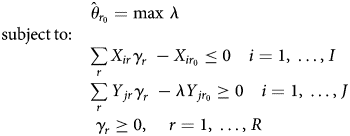
where Y jr is the amount of the jth output observed for the rth DMU, X ir is the amount of the ith input consumed by rth DMU and λ is a scalar value that seeks to expand all outputs proportionally given the input quantities. Then, the efficiency of DMU r 0 is the reciprocal of its inefficiency $\hat{\theta }_{r_0}$ , which is obtained by solving the linear programming problem in equation (1). The subscript γ r represents non-negative input/output weights that determine the best-practice frontier for the DMU r 0. In the same way, DEA computes weights for all DMUs in the sample.
The measure of technical efficiency evaluated using equation (1) assumes a constant return to scale (CRS) as introduced by Charnes et al. (Reference Charnes, Cooper and Rhodes1978) in their original DEA paper and is commonly known as ‘DEA-CCR’. However, the assumption of CRS is only suitable if all DMUs are operating at an optimal level. To integrate the requirement that not all DMUs may be operating at an optimal level, i.e. to incorporate the assumption of a variable return to scale (VRS) in the production, Banker et al. (Reference Banker, Charnes and Cooper1984) extended the study of Charnes et al. (Reference Charnes, Cooper and Rhodes1978) by introducing a convexity constraint:

DEA with a convexity constraint is known as ‘DEA-BCC’, ensures that an inefficient DMU is only compared against DMUs of similar size, thereby avoiding the issue of being benchmarked against DMUs that are substantially bigger or smaller.
A revolutionary application of bootstrap into DEA literature was introduced by Simar and Wilson (Reference Simar and Wilson1998) that applied homogenous bootstrap to DEA efficiency scores to correct for bias. The homogenous DEA bootstrap methodology also allows users to extract the sensitivity of efficiency scores which results from the distribution of (in)efficiency in the sample. In another study, a more sophisticated approach which Simar and Wilson (Reference Simar and Wilson2007) termed as algorithm 2, applied double bootstrap to a truncated regression to remove bias from the technical efficiency scores and analyse the effect of various variables on efficiency levels. A detailed technical explanation of Simar and Wilson (Reference Simar and Wilson1998, Reference Simar and Wilson2007) DEA bootstrap methodology can be found in Coelli et al. (Reference Coelli, Rao, O'Donnell and Battese2005). In this study, algorithm 2 of Simar and Wilson (Reference Simar and Wilson2007) is employed to estimate the technical efficiency scores of DHBs and how technical efficiency is associated with sizes and other factors.
However, with a large number of inputs and/or outputs relative to DMUs, DEA runs into the issue of the loss of discriminatory power, which incorrectly assigns all DMUs with very high-efficiency scores. Various studies show that as the number of input/output variables increase, the production frontier becomes defined by a larger number of DMUs, which leads to more DMUs being ranked as efficient, thereby reducing the ability of DEA to differentiate among DMUs (Adler and Golany, Reference Adler and Golany2001; Adler and Yazhemsky, Reference Adler and Yazhemsky2010). Another issue with DEA is the effect of highly correlated inputs on efficiency scores. A study by Dong et al. (Reference Dong, Mitchell and Colquhoun2015) showed that DEA scores are particularly sensitive to the correlation among input variables and, in some cases, have substantial influence over the discriminatory power of DEA.
To address these issues, Ueda and Hoshiai (Reference Ueda and Hoshiai1997) and Adler and Golany (Reference Adler and Golany2001) independently introduced the integration of PCA into DEA literature to assess the efficiency levels of DMUs. In both cases, the motivating factor in combining PCA and DEA was to increase the discriminatory power of the DEA when there is an excessive number of inputs/outputs compared with the number of DMUs. PCA overcomes the issue of excessive types of inputs relative to DMUs and the correlations among them by reducing the dimensionality of inputs. In support of PCA-DEA, Nataraja and Johnson (Reference Nataraja and Johnson2011) found that PCA-DEA performed relatively better among four different methods available in the literature with highly correlated inputs and small datasets (less than 300 observations) compared with all other methodologies.
PCA transforms high-dimensional data into a set of uncorrelated PCs, with the first few PCs retaining most of the variance in the original data. If the first few PCs describe 80–90% of the variance in the data, then the original variables can be replaced without much loss of information (Adler and Yazhemsky, Reference Adler and Yazhemsky2010). The new variables, commonly known as ‘PCs’, are weighted sums of the original data.
In this study, a model by Adler and Golany (Reference Adler and Golany2001) is used to motivate the setup of PCA. Let us assume a vector Z = [Z 1, Z 2, …, Z q], which represents the high-dimensional data that needs to be aggregated. The vector Z has a covariance matrix V with eigenvalues τ 1 ≥ τ 2 ≥ ⋅ ⋅ ⋅ ≥ τ q ≥ 0 and normalised eigenvectors l 1, l 2, …, l q. Then consider the following linear combinations with superscript t (transpose operator) that derive the PCs:
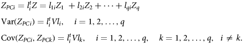
Then, the PCs: $Z_{PC_{1\;}}, \;\;Z_{PC_{2\;}}, \;\ldots , \;Z_{PC_{q\;}}$ are uncorrelated linear combinations ranked by their ability to explain variances in the original vector Z.
To illustrate DEA-PCA formulation, let $L_x = \{ {l_{ir}^x } \}$ be the matrix of the PCA linear coefficients of input data and $L_y = \{ {l_{jr}^y } \}$
 the matrix of the PCA linear coefficients of output data. Therefore, the PC scores X PC = L xX Lx and Y PC = L yY Ly are weighted sums of the corresponding original data X Lx and Y Ly.
Then, the output-oriented DEA-BCC model in equation (1) can be defined as:

The PCA-DEA set in equation (4) is based on the correlation rather than covariance as variables are often measured in different units. As a result, the PCs are solely based on the correlation matrix and do not require a multivariate normal assumption (Adler and Yazhemsky, Reference Adler and Yazhemsky2010).
If the efficiency analysis is limited to cross-sectional data, then the efficiency frontier is formed by DMUs operating in a given period, and the role of time cannot be incorporated into the analysis. When time-series data are available, one way to specify the DEA frontier is by pooling all DMUs from different periods, leading to an intertemporal DEA analysis. Under this analysis, a global technological frontier is constructed against which each DMU's efficiency performance is evaluated. An advantage of intertemporal specification in the DEA is that it avoids situations that may incorrectly penalise DMUs that demonstrate excessive use of resources intended to generate future benefits (Cullinane and Wang, Reference Cullinane and Wang2010). However, a caveat in the intertemporal specification emerges from the presumption that no significant technological progress occurred during the time period under consideration. Nevertheless, the intertemporal analysis does provide an opportunity in the context of DEA to examine trends in efficiency levels over time.
On the contrary to the assumption of no technological change over the entire time period, the contemporaneous DEA analysis assumes that technological change occurs in each time period. In other words, in contemporaneous analysis, a new frontier is assumed for every period against which ‘DMUs’ performances are compared. However, analysis of the efficiency performance trend under the contemporary approach is problematic, as comparisons of efficiency measures are based on different best-practice frontiers whose differences are not known.
Another dynamic variant of DEA called ‘window analysis’, was introduced by Charnes et al. (Reference Charnes, Clark, Cooper and Golany1984) to evaluate the efficiency of a United States Air Force base. The basic idea behind window-DEA is simple and based on the principle of moving averages, where DEA is applied successively on the overlapping periods of constant width, called ‘windows’ (Charnes et al., Reference Charnes, Cooper, Lewin and Seiford1994). An important decision in window analysis is the selection of window width. However, no straightforward methodology that aids in the selection of an appropriate window width exists and incorrect selection of window can lead to incorrect conclusions. In this study, an intertemporal DEA with two-stage bootstrap is used as a primary model to examine the trends in the performance over time. In order to conduct a sensitivity analysis of DEA scores, the two-stage bootstrapped technical efficiency scores are also computed for contemporaneous and window approach
5. Output and input data
The Ministry of Health (MoH), under the Official Information Act 1982, has provided data on DHB owned and operated hospitals for this study. The hospital data comprise yearly balanced panel data from the year ending June 2011 to June 2017 for all 20 New Zealand DHBs. Table A2 contains the variables and their definitions.
The health care sector is a multi-output industry where a wide range of health care proxies are used to account for heterogeneous health care services. This study, however, uses case-weighted inpatient discharges and price-weighted outpatient visits as outputs. The data weights inpatient discharges by case-weights to account for relative resource consumption and case complexity. Similarly, outpatient visits are price-weighted to account for differences for resources consumed by each DHB. Price-weighted outpatient data are calculated by multiplying outpatient volumes by the price of respective purchase unitsFootnote 3 and dividing the total figure by the national case-weight price.
The FTEs (Full-time equivalents) of medical, nursing, allied, support and management staff is used to account for labour inputs used by each DHB (Jacobs et al., Reference Jacobs, Smith and Street2006; Hollingsworth and Peacock, Reference Hollingsworth and Peacock2008; Hussey et al., Reference Hussey, De Vries, Romley, Wang, Chen, Shekelle and McGlynn2009). Regarding capital inputs, this study uses the value of capital asset value as a proxy for capital input (Grosskopf and Valdmanis, Reference Grosskopf and Valdmanis1993; Chattopadhyay and Ray, Reference Chattopadhyay and Ray1996). Capital asset value represents a broad range of capital consumed by health care. As a result, the end-of-year capital asset values of buildings, equipment (clinical and non-clinical), information technology and motor vehicles reported by DHBs is used as a proxy for capital input. This study also uses outsourced clinical costs associated with the patient's treatment as an input. Table 1 presents the basic statistics of all the input and output variables for 2011–2017. Concerning the DHB sizes, the data show that the average length of hospital stay in small DHBs is 2.79 days, followed by 2.75 days for medium DHBs, which is above the average. On the contrary, the average length of hospital stay for large-sized DHBs is 2.56.
Table 1. Descriptive statistics
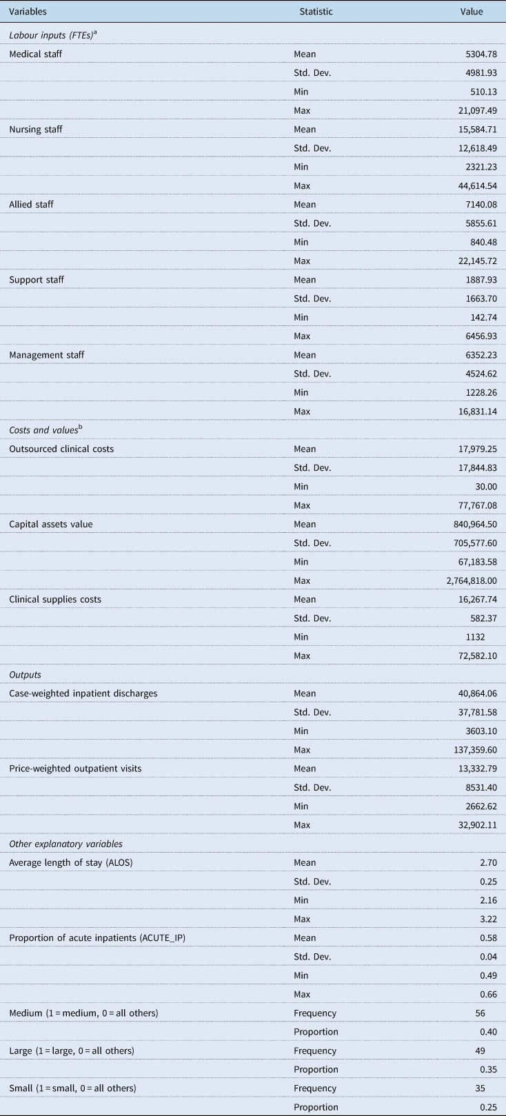
a One FTE is based on a person who works a 40-hour week. However, a person working more than 40 hours a week is only counted as one FTE.
b Costs and values are reported in thousands of New Zealand dollars.
6. Empirical illustration
As seen earlier, PBFF is used for the annual allocation of funds to each of New Zealand's 20 DHBs. Therefore, in any financial year, DHBs are given a fixed amount of resources subject to which they are expected to meet their population's health care needs. Thus, an output-oriented DEA model is employed to examine technical efficiency.
Another critical consideration is the scale size under which different DHBs operate. Because their large size may cause DHBs to operate inefficiently, they should only be compared with similar-sized other DHBs (Jacobs et al., Reference Jacobs, Smith and Street2006). This study uses a DEA model, introduced by Banker et al. (Reference Banker, Charnes and Cooper1984), which is appropriate in sectors where DMUs may not be operating at an optimal level due to various constraints. Therefore, the evaluated efficiency scores in our study reflect pure technical efficiency, which is an index to capture managerial performance.
In our dataset for a given year, there are eight inputs, two outputs and 20 DHBs, which clearly is not optimal and consequently, reduces the discriminatory power of DEA and leads to biased efficiency estimates. In this study, PCA is used to reduce the dimensionality of inputs into few uncorrelated PCs and replace the original inputs with PCs that explain at least 80–90% of the variance in the input data. The first step in the application of PCA-DEA to a dataset is the computation and selection of PCs. In PCA, PCs are prioritised in descending order based on the amount of explained variation in the original data. Table A3 presents the results of PCA by year. The first two PCs on inputs explain the majority of variance in the original input data; that is, these two PCs together explain more than 91% of the correlation in each of the seven years analysed. Consequently, the PC scores of the first two PCs from the input side can be used in place of the eight input types and run the DEA-BCC model with double bootstrap to evaluate the technical efficiencies and the effect of contextual variables.
To run DEA, the inputs and outputs are required to be strictly positive. Some of the linear coefficients of input can be negative and result in negative PC scores. Ali and Seiford (Reference Ali and Seiford1990) proved that an affine transformation could be used when the convexity constraint (DEA-BCC model) is imposed without altering the efficiency frontier. Furthermore, if output-orientation is used, then the DEA-BCC model is input translation-invariant (Pastor, Reference Pastor1996). Hence, a simple data transformation motivated by Adler and Golany (Reference Adler and Golany2001) is used, where the PC scores are added by the absolute value of the smallest negative number in the dataset plus one. This transformation can be represented as:

7. Empirical results
As stated earlier, the intertemporal two-stage DEA bootstrap methodology of Simar and Wilson (Reference Simar and Wilson2007) assuming a VRS is used as the primary model to discuss results in this section. However, the mean technical efficiency scores under CRS consumption is also displayed along with scale efficiency scores in Table 2 for additional insights.
Table 2. Estimates of mean technical efficiency scores
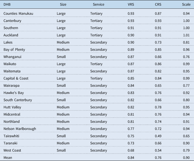
Estimates of average VRS technical efficiency scores in Table 2 show that all of the top four performing DHBs are large-sized and provide tertiary level hospital services. It is also noticeable that all four of these DHBs operate at a very high level of scale efficiency as they provide hospital services to high population areas. Besides, they also accept patients from other secondary DHBs who require tertiary-level hospital care. However, the other three large DHBs – Waikato, Waitemata and Capital & Coast, despite operating at high-scale efficiency have posted slightly lower levels of VRS technical efficiency scores compared with their counterparts – Counties Manukau, Canterbury, Southern and Auckland.
On the contrary, all nine lowest-performing DHBs based on their respective VRS efficiency scores are either small- or medium-sized and provide secondary level hospital services. The exceptions, however, are Lakes, Bay of Plenty and Whanganui DHBs who performed reasonably well compared to their similar-sized counterparts at the bottom. A Kruskal–Wallis H equality-of-population rank test is conducted to determine if the median VRS technical efficiency scores were different for the three sizes. The result shows that there is evidence of a statistically significant difference in the median efficiency scores between the three DHB sizes with χ 2(2) = 41.71 and p-value of 0.001. Furthermore, of the DHBs at the bottom, all except for West Coast, Tairawhiti and South Canterbury operate with a relatively high level of scale efficiency (above 0.90) (Table A4).
A quick look at the mean average length of hospital stay among three DHB size indicates that large ‘DHBs’ average stay is about 2.56 days, compared to medium and small, which has 2.75 and 2.79 days, respectively. The Kruskal–Wallis test resulted in a p-value of 0.0001 with the χ 2(2) = 21.86, which indicates that there is a statistically significant difference in the median average length of hospital stay days between the three different sizes. Therefore, higher average length of hospital stay might be a possible factor for lower VRS technical efficiency levels of medium and small-sized DHBs. In addition, Controller and Auditor-General have indicated that some DHBs delay the access of their patients to hospital facilities at tertiary DHBs in order to limit the outflow of DHB funds (Controller and Auditor-General, 2013).
On the contrary, the higher average length of stay among medium- and small-sized DHBs may be unavoidable as there may be other factors such as availability of primary health care services and other occupancy pressures that might affect the length of stay in hospitals. Therefore, the average length of stay in isolation may not thoroughly explain the low technical efficiency rates among small- and medium-sized DHBs.
The five poorest performing DHBs – West Coast, Taranaki, Tairawhiti, Nelson Marlborough and Northland deserves an explanation. Both West Coast and Nelson Marlborough DHBs have faced an acute shortage of clinical staff (Health Workforce New Zealand, 2015; West Coast District Health Board, 2017, 2018; ASMS, 2017a, 2017b). This results in heavy dependency on costly outsourced clinical personnel and raises costs which drive efficiency relative to other DHBs. On the contrary, both Tairawhiti (Ministry of Health, 2019) and Northland (Northland District Health Board, 2017, 2018) have a higher proportion of residents living in poverty compared to the national average and are known to have long-term health issues (Robson et al., Reference Robson, Purdie, Simmonds, Waa, Faulkner and Rameka2015). This leads to higher resource consumption and a more extended stay in hospital per patient, which is evident from the relatively high average length of stay of 2.91 in Tairawhiti and 2.87 in Northland compared to the national average of 2.69 days.
One of the benefits of using intertemporal DEA analysis is that it enables the observation of the trend in efficiency performance. The observed trends measure each DHB's ability in catching up to the frontier over the entire time period under consideration. In Figure A1, the VRS efficiency scores for each DHB is plotted against time and shows that most DHBs have an upward trend in their efficiency performance between 2011 and 2017. Among the DHBs with an upward trend, the performance of West Coast DHB is commendable, followed by Capital & Coast, Wairarapa and Waitemata who have shown a significant increase in their VRS technical efficiency over time. Nelson Marlborough DHB's performance, however, indicates a declining trend between 2011 and 2017. In comparison, the performance of Hawke's Bay, Northland, South Canterbury, Southern, Tairawhiti, Taranaki, Waikato and Canterbury results remained unchanged between 2011 and 2017. It is also important to note that none of the low-performing medium- and small-sized DHBs except for West Coast, Wairarapa and Hutt Valley has improved their efficiency performance between 2011 and 2017.
As the VRS technical efficiency scores presented in Table 2 is obtained through the application of double bootstrap to a truncated regression, the result of truncated regression is displayed in Table 3 as it offers some additional insights.
Table 3. Results from truncated regression with bootstrap
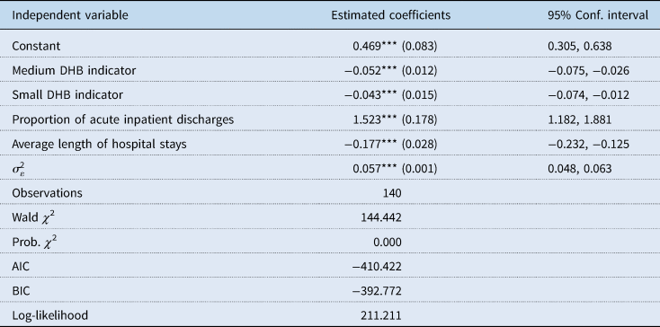
Figures in parentheses are bootstrap standard errors.
The coefficient estimation is undertaken in STATA using command simarwilson – Algorithm 2, with 2000 bootstrap replications.
***, **, * indicate significance at the 1%, 5% and 10% statistical levels, respectively.
The coefficients in Table 3 shows that being a small- and medium-sized does appear to have an association with a lower level of VRS technical efficiency scores. Furthermore, as expected, an increase in the average length of hospital stays is correlated with a decrease in VRS technical efficiency levels among DHBs. On the contrary, an increase in the proportion of acute inpatient is linked to an increase in VRS technical efficiency scores. Furthermore, there are various other variables that may affect technical efficiency performances of DHBs that simply cannot be incorporated in the current study due to the lack of comprehensive data and the limited number of observations. Furthermore, the quality of hospital service, a critical component of public health care is also missing.
Since this study uses the intertemporal DEA (I-DEA) analysis to evaluate the VRS technical efficiency, it would be interesting to assess whether the ranking of the DHBs substantially changes as the period under analysis changes. This is achieved by comparing the intertemporal VRS technical efficiency scores with the window-DEA (W-DEA) and contemporaneous (C-DEA) VRS efficiency scores. The W-DEA analysis requires the selection of a suitable window width where technology is assumed to be constant in each window. However, the technical change cycle of the New Zealand health system is difficult to observe, and little study has been done in the area of health technology diffusion among New Zealand DHBs (Allsopp, Reference Allsopp2006). However, Charnes et al. (Reference Charnes, Cooper, Lewin and Seiford1994) suggested a window width of three or four in general, which represents the best balance of informativeness and stability of the efficiency scores. Therefore, a window width of 3 years is used, which is a suitable neutral compromise to curtail the impact of technological changes during the time period of analysis. Furthermore, the impact of technological changes on the DHBs is gradual, such that in each of the 3-year windows the technological changes are not large enough to make comparisons within that window unreasonable. On the contrary, under the C-DEA approach, the technological frontier is assumed to be changing every year, which is an extreme assumption. The computed mean technical efficiency scores from all three models along with the Spearman rank correlation coefficients are displayed in Table 4. The technical efficiency scores for each DHBs by year under C-DEA and W-DEA approach is presented in Tables A5 and A6, respectively.
Table 4. Spearman rank correlation coefficients
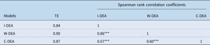
Note: TE is the abbreviation used to represent the measure of VRS technical efficiency.
***, **, * indicate significance at the 1%, 5%, and 10% confidence levels, respectively.
The results in Table 4 shows that obtained DEA scores from I-DEA and W-DEA have a high correlation coefficient of 0.86, implying that the ranking of DHBs is relatively consistent between these two models. However, the correlation between I-DEA and C-DEA is slightly lower at 0.57. Similarly, the correlation between C-DEA and W-DEA is only 0.60. This further implies the assumption of the new technological frontier for each year as assumed under contemporaneous DEA might not be a reasonable assumption.
8. Concluding remarks
This study is the first in the literature to use PCA and intertemporal DEA analysis together to study the dynamic performance behaviour of health care service providers across time using panel data. The main findings of this study are as follows:
(1) The average technical efficiency of New Zealand DHBs in delivering hospital services for the period 2011–2017 stands at 0.84 compared with the theoretical optimum.
(2) The trend in technical efficiency show that majority of large-sized DHBs have witnessed an improvement in their efficiency performance over time, whereas most medium- and small-sized DHBs has not improved their technical efficiency performance between 2011 and 2017.
(3) The top-performing DHBs are large, and provider tertiary level hospital services. These DHBs also operate at a very high level of scale efficiency. On the contrary, all of the poorest performing DHBs are small- and medium-sized except for Lakes, Bay of Plenty and Whanganui who performed comparably well.
(4) The average length of hospital stay among medium- and small-sized DHBs appear to be slightly high than that of large-sized DHBs. The results from truncated regression show that high average length of hospital stay negatively impacts technical efficiency levels of DHBs. Therefore, reducing the average length of hospital stay with quality hospital service might improve the efficiency of small- and medium-sized DHBs.
(5) The DHBs that experience a persistent shortage of clinical staff and operate in areas of high social deprivation appear to operate with a lower level of technical efficiency. However, a more in-depth analysis is required to draw any significant conclusions about the effect of these variables on technical efficiency levels.
Empirically, this study on New Zealand DHBs shows that PCA and DEA intertemporal analysis offers a simple and insightful way to assess efficiency where there is a limited number of DMUs relative to input/output types. This study hopes to pave the way for further analysis in other sectors/countries, where traditionally dimensionality has limited the application of DEA to study the trend of efficiency performance. However, there are many limitations to this study that is worth a mention. First and foremost, the absence of other contextual data that could have been used to assess its impact on technical efficiency levels. Second, the absence of the quality of inpatients and outpatients' services provided by DHBs. Third, the inability to incorporate the unobserved heterogeneity that might be captured as inefficiency. Nevertheless, it is hoped that the results of this study will attract the interest of policymakers in the potential insights to be gained from a more in-depth efficiency analysis of New Zealand's public health care system.
Conflict of interest
None.
Appendix A
Table A1. List of New Zealand DHBs
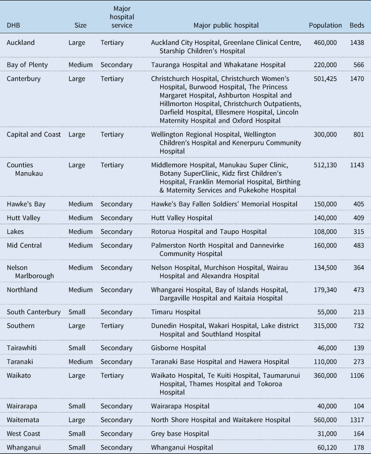
Table A2. Description of variables
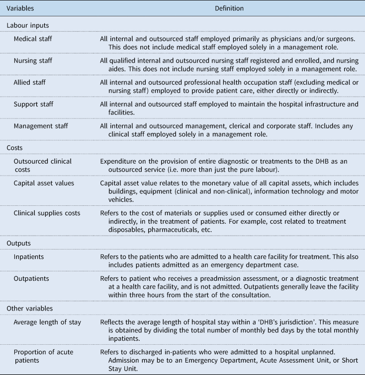
Table A3. PCA of DHB inputs based on the correlation
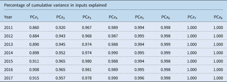
Table A4. VRS intertemporal technical efficiency scores

Table A5. VRS contemporaneous efficiency scores
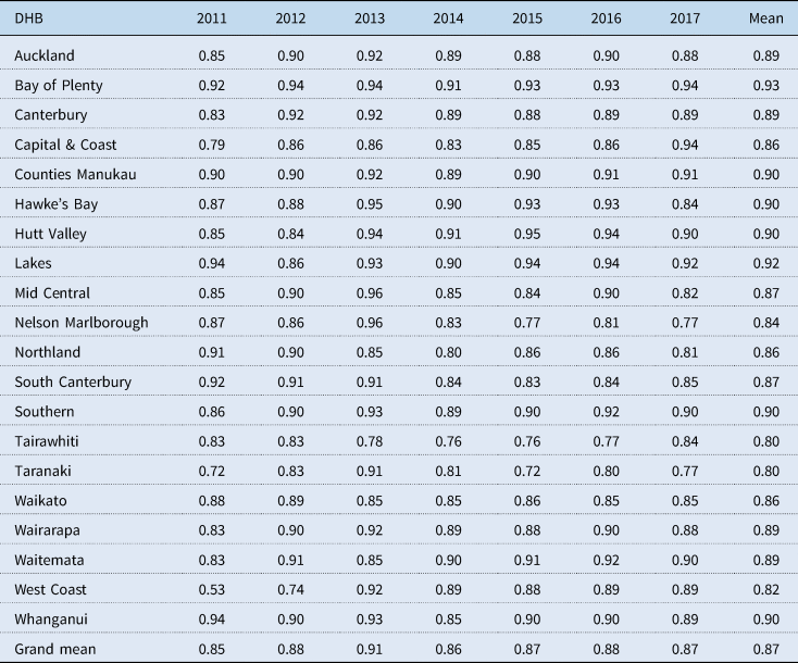
Table A6. VRS window efficiency scores
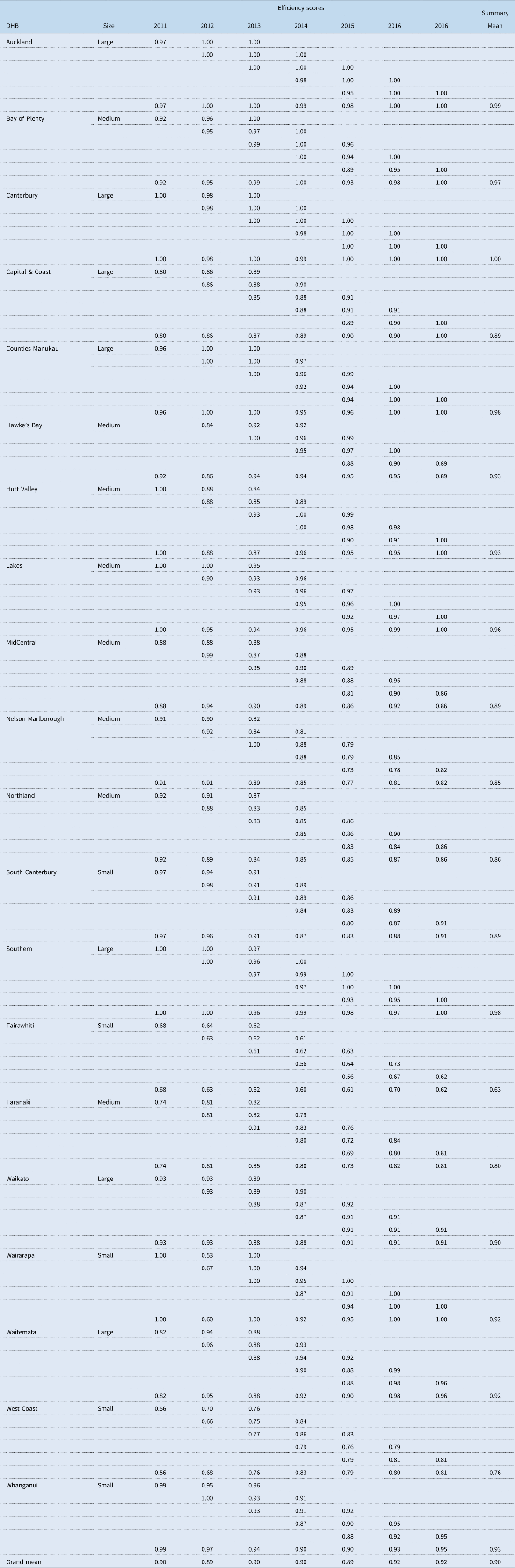

Figure A1. VRS intertemporal technical efficiency scores overtime.


