Conceptualizing and operationalizing party dominance

Any attempt to provide a clear definition (and operationalization) of dominance should start from a review of the main studies reflecting on this important aspect of party politics. Despite being relatively fragmented, the literature on dominance seems to focus on two key dimensions: absolute and relative dominance. A third element is time: that is, how long a party has been in power. However, the literature has tended to complicate the picture by imposing categories and thresholds, which are often arbitrary and, as a consequence, are continuously challenged. In addition, various definitions and operationalizations of dominance are mainly used for the selection of qualitative case studies and are difficult to apply to large-N analyses. The aim of this section is to develop a continuous measure of dominance which includes all the dimensions mentioned above.

One of the first definitions of dominant party was provided by Maurice Duverger (Reference Duverger1954). According to the French scholar, we have a dominant party when its ‘influence exceeds all others for a generation or more’, and its ‘doctrines, ideas, methods, its style, so to speak, coincide with those of the epoch’ (Duverger Reference Duverger1954: 308). This definition effectively captured some of the key aspects of dominance, although it did not provide clear indicators which would allow scholars to assess dominance empirically and develop quantitative comparisons across many cases.

Giovanni Sartori (Reference Sartori1976: 193) moved from Duverger’s starting point and proposed a simpler definition of dominant party:

Sartori also explicitly compared the largest ruling party to its main competitor in order to assess its level of dominance. He mainly referred to electoral returns rather than legislative strength, but the interesting point he made is that dominance is assessed in relation to the competition faced by the ruling party.

Sartori’s definitions of dominance and pre-dominance are central in Matthijs Bogaards’s (Reference Bogaards2004) study of dominant parties and party systems in Africa. Bogaards does not just consider the share of the votes but also refers to the share of the seats obtained by the ‘runner-up’. Therefore, the legislative strength of the largest competitor is explicitly taken into account when assessing the dominance of ruling parties. However, it is not clear how each factor considered by Bogaards – vote share, seat shares of winner and runner-up – contribute to an overall assessment of dominance. A consequence of not linking different indicators together is that it is not possible to rank parties from the most to the least dominant, since no single measure is provided. Things become even more complicated when we move from parties to party systems. Bogaards (Reference Bogaards2004: 288) criticizes ‘continuous measures’, such as the number of effective parties, and warns that they may suggest ‘relevant variation where there is none’. Yet the opposite is also true and indeed Bogaards, who mainly relies on Sartori’s definition, ends up considering as dominant systems those with ruling parties controlling between 48.9% and 100% of the parliamentary seats. Generally, the discrepancies and contradictions existing in the literature, also highlighted by Bogaards, seem to derive from a tendency to convert quantitative, continuous indexes into qualitative, categorical typologies (and vice versa). To avoid these contradictions, this article aims to provide a multidimensional, continuous measure of dominance, without setting any categorical classification based on qualitative aspects of party competition. The two strategies may be complementary but should not overlap. One may rely on a mixed-method strategy (Lieberman Reference Lieberman2005) and use continuous quantitative measures to identify interesting cases of party dominance, which could then be qualitatively analysed.

T.J. Pempel’s (Reference Pempel1990: 3–4) definition seems more compatible with the development of a continuous measure of dominance. He argues that one key aspect of dominance is that a party must be dominant in number. This means that it should win a larger number of seats than its opponents. Interestingly, Pempel does not set a specific threshold beyond which we can categorize a party as dominant but just refers to a ‘plurality’ of seats. Another important aspect of this definition is that it excludes minor parties involved in governing coalitions. Of course, these minor parties may play an important, pivotal role, since they may be necessary for the formation of a government (winning) coalition (Bolleyer Reference Bolleyer2007). However, given their role as junior coalition partners of a larger party, they can be defined as a dominance enabler, rather than dominant. Indeed, they may be crucial in keeping larger parties in government and helping them preserve their dominant role in the party system.

Two other factors identified by Pempel may be important for the development of a measure of dominance: governmental dominance and chronological dominance. In order to be dominant, a party has to be at the core of the government over a substantial period of time. This last point adds a ‘dynamic’, ‘longitudinal’ aspect to the definition of dominance. Again, no threshold is set, and this is quite crucial if, instead of providing rigid categories, we want to measure dominance on a continuum. The importance of adding a time dimension to dominance, without imposing discrete categories, is also underlined by Jingjing Huo (Reference Huo2005).

However, Huo’s definition deviates from Pempel’s one in respect of governmental dominance. Huo identifies two dimensions of dominance – electoral and governmental – and also calculates scores of dominance for parties that have never been in power. This article opts for the definition provided by Pempel and focuses on the largest ruling parties. Indeed, it would be problematic to assess the dominance of political forces that have not even been able to control the executive at least once over a relatively long period of time. Generally, extending the concept of dominance to junior coalition parties and parties in permanent opposition may result in conceptual ‘overstretch’ (Sartori Reference Sartori1970).Footnote ² Political dominance would lose its analytical utility if used interchangeably with political relevance, because the latter concept applies to a much larger number of parties. If we stick to Pempel’s definition, only a subgroup of relevant parties, namely the largest ruling parties across different polities, will be assessed, compared and ranked in terms of their dominance. All other parties may still be assessed as more or less relevant rather than dominant.

Based on the above discussion of various definitions and operationalization strategies, it is possible to identify two key dimensions of dominance. The first dimension is the absolute dominance of the main ruling party. The larger the share of seats such a party controls in parliament, the more dominant this party will be in the legislative process. This aspect is also included by Huo (Reference Huo2005: 746) in his operationalization of ‘electoral dominance’. However, Huo does not consider the fact that the dominant role of a party also depends on the strength of its main competitor. Indeed, a strong opposition party (or coalition partner if the main competitor is also a ruling party, as happens in the event of a grand coalition) would place more pressure on the main ruling party than a small competitor. Thus, absolute dominance tells us only part of the story and is not very meaningful if it is not combined with relative dominance. For instance, there is a big difference between a ruling party controlling 55% of the seats with its main competitor being at 45% and a ruling party still controlling 55% of the seats with the largest competitor winning only 25% of the seats. Equally, relative dominance should not be considered as a sufficient indicator of dominance. Again, a ruling party with twice as many seats as its main competitor would clearly be more dominant if its absolute share of seats was 60% rather than only 30%.

Since the meaning of each of the two dimensions identified above depends on the other, it makes sense to multiply them (Goertz Reference Goertz2006: 95–128) to obtain a measure of ruling party dominance within a legislature. We can also say that relative dominance is weighted by the absolute share of seats that the main ruling party obtains. The formula to calculate dominance is summarized thus:

$$Dominance\,(d)\;{\equals}\;Absolute\;{\asterisk}\;Relative\;{\equals}\;s\;{\asterisk}\;\left( {{{s{\rm }} \over c}} \right)$$

Where s is the share of parliamentary seats controlled by the largest party in government and c is the share of parliamentary seats controlled by its main competitor, which can either be an opposition party or a coalition partner (in the case of grand coalitions). When a party moves into opposition, it is no longer the largest governing party and its d will equal 0.

Yet d only provides a score of dominance at a single point in time (i.e. one particular year) but does not tell us how dominant a party has been over a substantial period of time (several years). The time dimension of dominance is taken into account by calculating the average dominance score of a party that has been in government at least once over a defined period of time. Therefore an overall measure of party dominance (D instead of d) is given by the following formula:

$$Overall\,Dominance\,\left( D \right)\;{\equals}\;{\rm }{{\sum_{i{\equals}1}^n d} \over t}$$

Yearly d scores are added up and then divided by the number of years of the period considered (t). This is basically an average since, when we calculate the overall dominance of a party, the number of its d scores (n) corresponds to t.

It should be highlighted that party dominance is conceptually different from (although it might be related to) electoral vulnerability. This concept was developed and operationalized by Ellen Immergut and Tarik Abou-Chadi (Reference Immergut and Abou-Chadi2014) and is based on two dimensions: electoral pressure and political protection. The first dimension, which includes volatility, disproportionality, effective number of parties and fraction of electoral winners, may be causally linked to dominance. For instance, systems characterized by low levels of volatility and high disproportionality of the voting system may have a positive impact on party dominance. Yet including these aspects in a definition of dominance would risk conflating causes and effects. The second dimension, political protection, which considers the size of governmental majority in relation to the number of governing parties, comes closer to the definition of dominance that is developed here. Yet this measure ignores the relationship between the largest governing parties and its main competitor (i.e. relative dominance). It might be that the governing coalition has a very small majority (or is even a minority government), but it manages to stay in power because the opposition is highly fragmented and the main opposition party obtains considerably fewer seats than the largest governing party and is unable to coalesce with other opposition parties.

This study focuses on party dominance at the subnational level. This aspect has often been neglected by literature on party dominance, which is still clearly influenced by what has been defined as ‘methodological nationalism’ (Jeffery Reference Jeffery2008). The scant attention paid to the subnational dimension is surprising given the variation existing within countries, which is even greater than across countries. Comparing different regions within the same country would also allow to control for ‘statewide’ institutional, economic, political and social characteristics and focus on a limited number of region-specific variables to explain the causes or effects of dominance. Additionally, as shown in the following sections, political dynamics are usually more fluid at the national level, particularly in advanced democracies, and parties are more able to exert long-term control of government in some subnational contexts. Therefore, high levels of dominance are more typical of municipalities and regions than countries. It should also be noted that the strengthening of the regional level of government, the rise of the so-called ‘meso’, has been qualitatively and quantitatively assessed by several studies (Hooghe et al. Reference Hooghe, Marks and Schakel2010; Keating Reference Keating2013) and has attracted increasing attention from scholars focusing on quality of government (Argerberg Reference Argerberg2017; Charron et al. Reference Charron, Dijkstra and Lapuente2014; Putnam Reference Putnam1993). Therefore, an exclusive focus on the national dimension would neglect important territorial shifts in political and policymaking processes. This, however, does not mean that the measure developed here could not be applied to countries or regions beyond those of the three countries included in this article. In fact, one of the positive aspects of this index is that it can be used for a much larger number of cases at different levels of government below or above the regional one. In some respects, this study already applies the index to different levels, since its empirical analysis also considers the association between regional and national dominance.

In the existing literature, only the edited volume by Matthijs Bogaards and François Boucek (Reference Bogaards and Boucek2010) includes two chapters considering regional dominance. One by Amir Abedi and Steffen Schneider (Reference Abedi and Schneider2010) focuses on the Canadian provinces and German Länder; the other one, by Gordon Smith (Reference Smith2010), focuses on the Bavarian Christian Social Union (CSU) as a case of a regionally dominant party. Key aspects of Abedi and Schneider’s analysis are the focus on seats, rather than votes, controlled by ruling parties at the regional level, the development of a quantitative measure of relative dominance (the ‘power’ dimension) and the addition of a time dimension of dominance. However, rather than creating a single, continuous measure of dominance including both dimensions, the two authors rely on power and time to define different categories of dominance, which are not applied to a quantitative analysis but are only used for the selection of qualitative case studies.

In the same book, Jean-François Caulier and Patrick Dumont (Reference Caulier and Dumont2010) do not directly assess dominance of an individual party over a certain period of time but focus on the party system and provide two indexes which measure the effective number of relevant parties (ENRP) and the maximum contribution index of fragmentation (M) after a single election. In the same way as the index presented here, their indexes focus on legislative seat shares and are refinements of more traditional indexes of fragmentation (particularly Laakso and Taagepera Reference Laakso and Taagepera1979). Yet their empirical application is limited to systems that are already well known as being characterized by high levels of dominance (Sweden and Ireland between 1970 and 2006). Lastly, they admit the difficulty of averaging their indexes over a defined period of time (in fact, they do not consider number of years but elections) and, as a consequence, do not directly incorporate a longitudinal dimension in their measure of dominance.

The next section shows that one of the advantages of D is that different levels of dominance across a large number of regions are assessed through a single, but multidimensional, measure which can also be used in explanatory quantitative analyses. It should be highlighted that this article focuses on systems in which the government depends on a majority vote in the legislative body.Footnote ³ This decision is based on the fact that the overwhelming majority of European countries and regions can be classified as parliamentary systems. Application of the index to presidential systems is mentioned in the conclusion as a possible future development.

Party dominance in Italian, Spanish and German regions

D is now applied to the main ruling parties of 54 Italian, Spanish and German regions in the period from 1995 to 2015.Footnote ⁴ The total number of parties included in the sample is 95. As an example, the Appendix reports the calculation of dominance scores for the Social Democratic Party of Germany (SPD) and the Christian Democratic Union (CDU) in Lower Saxony (Table A1). The average of the dominance scores over the 21-year period is 0.302 for the SPD and 0.321 for the CDU.

D scores of all 95 parties are in the third column of Table A2 (in the Appendix). The top 10 of the ranking includes three regionalist parties of the so-called ‘Alpine’ macro-region (Caramani and Mény Reference Caramani and Mény2005): the South Tyrolean People’s Party (SVP), the Valdostan Union (UV) and the CSU. We also find the regional branches of the Italian Democratic Party (PD), the successor of the post-communist party, which in 2007 merged with left-wing Christian Democrats (Vampa Reference Vampa2009).Footnote ⁵ This party is particularly strong in Tuscany, Emilia Romagna and Umbria, which are characterized by a left-wing ‘political sub-culture’ (Trigilia Reference Trigilia1986). Finally, the regional branches of two statewide conservative parties are also included in this top list: the CDU in Saxony and the Spanish People’s Party (PP) in Murcia, Castile and Leon, and Galicia.

As stated above, the aim of this study is not to provide categorizations and thresholds, which may be seen as arbitrary. Rather, D places dominance on a continuum and lacks an upper boundary. It is multidimensional and can be easily applied to quantitative analysis, as shown in the examples provided in later sections of this article. However, it is not clear how D scores can be used in mixed-methods studies. Indeed, setting specific thresholds and boundaries may become particularly relevant for case selection when qualitative analysis follows, and complements, quantitative analysis. One way to address this issue is to look at the distribution of the cases included in the sample and, for instance, consider the scores within the upper quartile as ‘high dominance’, those in the interquartile range as ‘medium dominance’ and those in the lower quartile as ‘low dominance’. Table 1 shows the range of values for each group within the sample.

Table 1 High, Medium and Low Levels of Dominance Based on Sample Distribution

Note: PP=People’s Party.

Weighting dominance scores and comparing D with other measures

As shown above, the overall dominance (D) of a particular party is calculated by dividing the sum of its yearly dominance scores (d) by the number of years of the period considered (t). Since a party is assigned a d score of 0 for each year in opposition, the longer the party stays in opposition during t, the lower its overall D. Conversely, D will tend to be higher for parties that have spent most of t in government. It may be argued that this formula, despite including a time dimension, does not account for the fact that each additional year of continuous government contributes to consolidating the dominant position of a party. A refinement of the index of dominance could take into account this particular aspect by assigning different weights to each d score. Of course, this strategy should be carefully considered because the decision to introduce different weights could be seen as arbitrary and could be challenged by other scholars.

A possible solution would be to multiply each d by an increasing factor. The first d of the series could be multiplied by just 1, the next one by a higher factor, the one after by an even higher factor and so on until the party loses its governmental position. By how much should the factor increase? This study covers the period from 1995 to 2015. The total number of years (t) is 21, but if we consider 1995 as year 0 of the series, then the last year (2015) will be number 20. Therefore, each additional year could lead to a 1/20 (0.05) increase in the value of the weighting factor. This means that the first d of the series can be simply multiplied by 1, the second one by 1.05, the third one by 1.10 and so on. If a party stays in government for the whole period (from 1995 to 2015) the last d will be multiplied by 2, thus being weighted twice as much as the first d in the series. Of course, if a party loses the election and goes into opposition but then returns to power, the series would start again from 1. In this way, the weighting would ‘reward’ continuity in power.

The weighting formula can be summarized as follows:

$$Weighted\,Dominance\,\left( {wd} \right)\;{\equals}\;d{\rm \;{\asterisk}}\;\left[ {1\;{\plus}\;\left( {{1 \over {t{\minus}1}}} \right){\rm \;{\asterisk}}\;g} \right]$$

Where d is the yearly score of dominance of a party, t−1 is the total number of years of the period considered minus one because the first year is the starting point of the series. Finally, g is the number of years the party has continuously been in government during the period considered. As in the case of D, an overall (weighted) measure of dominance (WD) is obtained by dividing the sum of wd scores by the total number of years (t) of the period studied.

As an example, WD is calculated for the SPD and CDU in Lower Saxony between 1995 and 2015 (Appendix Table A3). Compared with D, the 1995–2015 WD of CDU increases by 0.07 while the SPD’s WD increases by less than 0.05. The difference is quite small. Yet since the SPD’s governmental experience was interrupted while the CDU was continuously in government for 10 years (2003–12), the score of the former increases by a smaller margin (16%) than that of the latter (22%). Of course, the difference between original and weighted scores is much more noticeable for parties at the top of Table A1 (see last column), which have been in power for the whole period. Yet changes in the ranking are minimal. Within the top 10 only the Galician PP would be replaced by the PP in Madrid.

Table 2 shows that D and WD are strongly (almost perfectly) correlated (r=0.995) and this points to the fact that the original score already captures important aspects of the time dimension. The table also provides an overview of the correlation between D and other measures that are often used to assess party system or individual party’s dominance. It can be seen, for instance, that this measure is significantly correlated to the effective number of parties (ENP) developed by Markku Laakso and Rein Taagepera (1979). The association is negative since, as expected, in more fragmented party systems, it is more difficult for a single party to establish a clearly dominant position. Yet the association is not very strong. This is because the ENP does not really measure dominance. A party may be more dominant when faced by a highly fragmented opposition. For instance, the SVP, the most dominant party in our sample, has consolidated its position in a context of moderate fragmentation which mainly affected the opposition in South Tyrol. In Lower Saxony, on the other hand, despite competing in a party system that is less fragmented than the South Tyrolean one, neither the CDU nor the SPD achieved high levels of dominance.

Table 2 Correlation between Overall Dominance (D), Overall Weighted Dominance (WD) and Alternative Measures

Notes: * p<0.01. D=overall dominance; WD=overall weighted dominance; ENP=effective number of parties; ENPD=effective number of parties with dominance (Taagepera Reference Taagepera1999); GD=governmental dominance.

More recently Taagepera (Reference Taagepera1999) provided a new measure to take into account the existence of a dominant party. This measure (ENPD) can be applied to the largest parties in regional government. It can be seen that, compared with ENP, the correlation with D is much stronger because ENPD better captures dominance. Of course, it is still negative because the higher the absolute dominance of a party, the lower its ENPD (since ENPD=1/p, where p is the share of seats controlled by the largest party).

Lastly Table 2 includes the measure of governmental dominance (GD) provided by Huo (Reference Huo2005). This measure focuses on the length of government tenure and bargaining strength of a party and, unlike ENP and ENPD, explicitly considers the ‘temporal’ dimension of government. GD correlates positively and rather strongly with both D and WD but is weakly correlated with ENP and ENPD. This may be due to the fact that GD is not clearly linked to the electoral dimension, as admitted by Huo himself. At the same time, both ENP and ENPD ignore the time dimension of dominance and focus on the ‘party system’ rather than individual parties.

A proof of the validity of D is that it is significantly correlated with all its main alternatives (including WD), even though such alternatives are not consistently correlated with each other. Therefore, it seems that it effectively captures different dimensions (electoral, governmental, temporal), which are often difficult to reconcile.

Application of the index: an example

D can be used to provide a preliminary explanation of why some ruling parties are more dominant than others at the regional level.Footnote ⁶ Variation in dominance may depend on various factors. This article includes an exploratory quantitative analysis as an example of application to hypothesis testing. For instance, it can be hypothesized that dominance at the regional level depends on how dominant parties are at the national level. The case of the Christian Democratic Party (DC) in Italy between 1970 and 1990 is a good example of a party that was also able to control the governments of most Italian regions firmly while being nationally dominant.

The positive association between national and regional dominance, however, may be dependent on the level of economic development of a region. The existence of interactions between regional attributes such as identity, distinctiveness or territorial mobilization and economic development has already been shown by studies focusing on regional governance (Keating and Loughlin Reference Keating and Loughlin1997; Tatham and Thau Reference Tatham and Thau2014). Yet less attention has been paid to how statewide dominance is mediated by territorial economic factors. It can be hypothesized that poorer regions are more dependent on centrally allocated resources and, as a consequence, tend to reward those parties that are in power at the national level. Again, the case of the DC is quite useful, since it tended to perform much better in the poorer regions of southern Italy (Leonardi and Wertman Reference Leonardi and Wertman1989). The Spanish Socialist Party (PSOE) during its period of dominance under the leadership of Felipe González established its political stronghold in Andalusia (Bukowski Reference Bukowski2002), one of the poorest Autonomous Communities, which was heavily reliant on the resources allocated by the central government. Takashi Inoguchi (Reference Inoguchi1990) suggests that difficult economic conditions may in fact favour parties that are nationally dominant, particularly in a context of high dependence from centrally allocated resources. On the other hand, the effect of national dominance may be more moderate, or even negative, in wealthier regions, which may be more inclined to challenge central redistribution of resources. Additionally, socioeconomic development may lead to the emergence of post-materialist values (Inglehart and Welzel Reference Inglehart and Welzel2005) and, as a consequence, the tendency to show less deference to dominant political elites at the national level and opt for political alternatives.

D can also be calculated for parties in government at the national level. So, for instance, in Spain, the PSOE has a national D score of 0.224, the PP has a score of 0.441, the regionalist party Convergence and Union (CiU) has a score of 0 (since it has never been in central government), in Germany the SPD has a score of 0.17, and so on.Footnote ⁷ Table 3 shows the results of a relatively simple linear regression model, which also includes country fixed effects to account for different institutional arrangements and country-specific traditions. The ideological orientation of a party on the left–right spectrum is also considered by relying on a simple dummy variable (centre-left=1; centre and centre-right=0). Model 1 shows that the coefficients of both national dominance and regional per capita GDP (both variables are also average values over the period 1995–2015) are positive and statistically significant at 0.05 and 0.01 levels.

Table 3 Explaining Party Dominance at the Regional Level: A Preliminary Model

Notes: * p<0.1; ** p<0.05; *** p<0.01. Standard errors in parentheses.

However, the effect of GDP on regional dominance is negatively affected by national dominance (and vice versa). Indeed, the interaction effect is negative and statistically significant at 0.05, meaning that parties that are nationally dominant are less able to establish their dominance in richer regions. This can be seen clearly in Figure 1, which is based on predicted values (based on the model) and shows that the association between GDP and regional dominance is positive for a party that from 1995 to 2015 has never played a dominant role at the national level (score=0), whereas it becomes negative for a party scoring 0.5 in national dominance and even more negative for a party that has been highly dominant in central government (score=1).

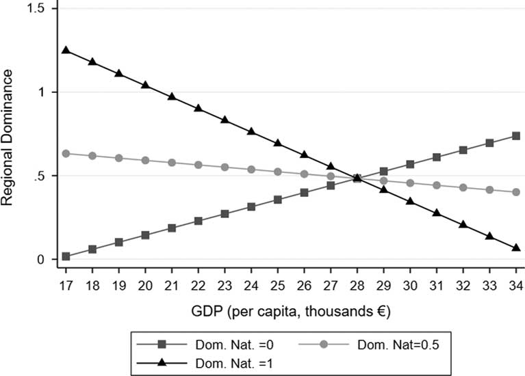
Figure 1 Effect of GDP on Party Regional Dominance Depending on Level of Party National Dominance

Model 2 excludes the country dummies because they are not statistically significant. This seems a good choice since the adjusted R-squared of Model 2 actually increases. Yet, rather than country-specific legacies, party-specific legacies may still play an important role. If we focus on the period from 1995 to 2015, we might hypothesize that parties that dominated regional politics in the previous period (1974–94) may rely on party allegiances that have consolidated over the decades. When we add the legacy control variable, the adjusted R-squared increases substantially from 0.085 to 0.411, meaning that previous levels of dominance may explain a great part of the variation in more recent years. However, our key independent variables remain statistically significant and this confirms that national political dynamics, interacting with territorial variation in economic development, play an important role in explaining different patterns of regional dominance. Future studies may test additional explanations – focusing, for instance, on different voting systems and cleavage structures – by using the index of party dominance presented here and developing more complex statistical models.

Lastly, it should be noted that results of the regression analysis presented in Table 3 would not significantly change if WD was used instead of D as dependent variable.Footnote ⁸

Aggregating dominance

Once individual party scores have been calculated, how can we obtain an overall measure of party dominance for a region? In this case our unit of analysis is no longer the individual party but a polity (the region). The challenge is to aggregate individual party scores in order to compare regional political systems and see which have been characterized by more dominant ruling parties. In order to do so, we need to develop an aggregation strategy that takes into account differences between regions which, over a defined period of time, have been ruled by one party with a large D and others ruled by two (or more) parties alternating in government with smaller D scores.

A simple sum or average of individual party scores would not be adequate. This can easily be shown by the following example. A study focuses on four regions over a period of 10 years. We want to rank them according to the level of dominance of their governing parties. In Region 1, only one party has been the largest one in government with a D of 1. In Region 2, we have two parties alternating in government and each scoring 0.5. In Region 3 we also have two alternating parties but one, with a D of 0.9, has clearly been more dominant than the other, which receives only 0.1. Lastly we have a region in which three parties have alternated as the largest ones in government, scoring 0.3, 0.3 and 0.4. If we simply added the individual D scores we would obtain an aggregate score of 1 in all cases, even though Region 1 was ruled uninterruptedly by one party and Region 3 had a more clearly dominant party than Regions 2 and 4. If instead we decided to calculate the average, the main problem would be that Regions 2 and 3 would receive the same overall score (0.5).

The least squares index used to measure disproportionality (Gallagher Reference Gallagher1991) includes some elements that might also be helpful for the construction of an index that aggregates dominance scores of individual parties while capturing the cross-regional differences highlighted above. In the case of disproportionality, the vote–seat differences of each party are squared, summed and divided by two. Lastly, the square root of the result is taken. In our case we are not dealing with deviations between votes and seats and therefore we do not need to calculate differences and divide the sum of squares by two. However, the logic behind Michael Gallagher’s index is that the square root of a sum of squares will tend to be greater when we have few large deviations than when we have many small deviations. Similarly, if we used the square root of the sum of squares, regions with few parties having large D scores would tend to receive a greater overall score than regions with many parties having small D scores. Therefore, the following formula may be used to aggregate individual party scores for a regional system:

$$Aggregate\,Regional\,Dominance\,\left( {ARD} \right)\;{\equals}\;\sqrt {\mathop \sum\limits_{i{\equals}1}^n D^{2} } $$

Where D is the overall dominance score of each party. Going back to our previous example of four regions, we would obtain the following results:

$${\rm Region}\,1\,\colon\,{\rm ARD}\;{\equals}\;\sqrt {1^{2} } \;{\equals}\;1$$

$${\rm Region}\,2\,\colon\,{\rm ARD}\;{\equals}\;\sqrt {0.5^{{2 }} \;{\plus}\;0.5^{{2 }} } \;{\equals}\;\sqrt {0.25\;{\plus}\;0.25} \;{\equals}\;\sqrt {0.5} \;{\equals}\;0.71$$

$${\rm Region}\,3\,\colon\,{\rm ARD}\;{\equals}\;\sqrt {0.9^{{2 }} \;{\plus}\;0.1^{2} } \;{\equals}\;\sqrt {0.81\;{\plus}\;0.01} \;{\equals}\;\sqrt {0.82} \;{\equals}\;0.91$$

$${\rm Region}\,4\,\colon\,{\rm ARD}\;{\equals}\;\sqrt {0.3^{{2 }} \;{\plus}\; 0.3^{{2 }} \;{\plus}\;0.4^{{2 }} } \;{\equals}\;\sqrt {0.09\;{\plus}\;0.09\;{\plus}\;0.16} \;{\equals}\;\sqrt {0.34} \;{\equals}\;0.58$$

With this method, Region 1, where only one party has been the main ruling party over the period considered (with a D of 1), obtains the highest score. The second largest score goes to Region 3, which has two D scores, but one clearly larger than the other and very close to that of Region 1. Then we have Region 2, where we have two main parties alternating in power with equal dominance. Finally the lowest score goes to Region 4, where, over a period of 10 years, three parties have played the role of largest ruling party and have obtained relatively low dominance scores.

Table A4 in the Appendix shows the ARD scores of the 54 regions considered in this study. The last column of the table also includes the difference between individual regional scores and the national score (calculated by using the same formula). It can be seen that most regions (42 out of 54) display ARDs that are higher than those at the national level (the difference is positive). This seems to confirm what Abedi and Schneider (Reference Abedi and Schneider2010: 77) suggest in their study of Canadian provinces and German Länder: ‘dominant party regimes are more frequent in … sub-national jurisdictions than in the capital cities’. Only some southern Italian regions (plus Friuli Venetia Giulia), Aragon, Cantabria, Berlin and Schleswig-Holstein have lower scores than their national systems. Interestingly, Italian regions are the majority in both the top 10 and bottom 10 in the ARD ranking and this seems to reflect some of the well-known differences existing between the north and the south of the country (Vassallo Reference Vassallo2013). These data also suggest that, generally, regional governments tend to be more stable and more firmly controlled by ruling parties than national governments.

The ARD score can be used as an independent variable to explain variation in institutional performance of regions. So far, a clear measure of political dominance has not been used in studies focusing on ‘quality of government’ (see Charron et al. Reference Charron, Dijkstra and Lapuente2014). Again, a simple model is developed here in order to provide an example of how this measure can be applied to empirical studies in political and social sciences. We can test whether quality of government (QoG) tends to be higher (or lower) in those regions where overall dominance of ruling parties has been greater. We assume that QoG is the outcome of a medium- to long-term process (Putnam Reference Putnam1993). Therefore, it makes sense to test whether today’s QoG is linked to political, economic and institutional factors that have been in place over a period of around two decades (from 1995 to 2015).

Regional QoG, the dependent variable, is measured by relying on the European QoG Index (EQI) developed by Nicholas Charron, Lewis Dijkstra and Victor Lapuente (Reference Charron, Dijkstra and Lapuente2014), ranging from 0 to 100, with higher scores indicating regions with higher-quality government.Footnote ⁹ Charron et al. also present a multiple linear regression model aimed at explaining cross-regional variation in EQI. An updated version of the model may also include our ARD, as the key independent variable to test the hypothesis that regions with more dominant ruling parties are also characterized by better institutional performance. Among the control variables that Charron et al. (Reference Charron, Dijkstra and Lapuente2014) consider, we have human development and institutional autonomy enjoyed by a region. The former variable is measured by the Human Development Index (HDI) developed by Sjoerd Hardeman and Lewis Dijkstra (Reference Hardeman and Dijkstra2014), which ranges from 0 to 100, with higher values suggesting higher levels of socioeconomic development (covering various dimensions such as income, health and education).Footnote ¹⁰ Regional autonomy is measured by relying on the Regional Authority Index (RAI) developed by Liesbet Hooghe, Gary Marks and Arjan Schakel (Reference Hooghe, Marks and Schakel2010). Charron et al. (Reference Charron, Dijkstra and Lapuente2014) also hypothesize that regional QoG may be associated with the size of a region operationalized in terms of population and surface, although they do not predict a clear direction of this association.Footnote ¹¹ They use the logged transformation of both variables, since their distribution is highly skewed and wide. Lastly, we should account for country-specific factors by introducing country fixed effects (reference category: Italy).

Table 4 shows that the model accounts for 82% of the variation in quality of government. Interestingly, our ARD index is positively associated with the dependent variable. One point increase in aggregate dominance is expected to result in an average increase of almost five points in QoG, holding all other independent variables constant, and this effect is statistically significant at 0.05. This means that regions with governments led by more clearly dominant parties are characterized by better-performing institutions regardless of their socioeconomic situation, level of autonomy, population, size and country-specific factors. Coefficients of control variables, such as HDI and population, are statistically significant at 0.01, whereas institutional autonomy, measured by the RAI, is statistically significant at 0.1. Human development, regional authority and surface of the regions are positively associated with the quality of government (although the coefficient of the latter variable is not statistically significant). On the other hand, population size seems to have a negative effect on the dependent variable. Finally, country fixed effects are not statistically significant.

Table 4 Explaining Variation in Regional Quality of Government (measured as EQI): OLS Model Including Aggregate Regional Dominance (ARD) as a Key Independent Variable

Notes: ** p<0.05; *** p<0.01. Standard errors in parentheses.

Of course, this is just an example of how the new index could be applied to a relevant research question. Despite the results shown in the quantitative analysis, this article does not provide a normative framework – which would require a deeper theoretical discussion – and does not argue that party dominance is desirable in all contexts. More evidence is needed to reject (less optimistic) hypotheses that link dominance to corruption, party infighting and decline in governmental responsiveness. In addition, the results discussed here do not tell us anything about the causal direction of the positive association between ARD and EQI. Again, starting from the preliminary results presented here, future studies could shed more light on the effects of party dominance on the effectiveness of subnational and national institutions.