


1. Introduction
The initiation of Himalayan uplift occurred at c. 50 Ma when India and Eurasia collided (Matthews et al. Reference Matthews, Dietmar Müller and Sandwell2016). The Indus River subsequently formed, carrying sediment from the Western Himalaya, Karakoram and Hindu Kush, and depositing it in the Indus Fan in the Arabian Sea (Clift et al. Reference Clift, Shimizu, Layne, Gaedicke, Schl Ter, Clark and Amjad2000, Reference Clift, Lee, Hildebrand, Shimizu, Layne, Blusztajn, Blum, Garzanti and Khan2002; Briggs, Reference Briggs2003). Provenance studies indicate that the Indus River and its associated tributaries have primarily fed the fan since the collision of India and Eurasia (Clift et al. Reference Clift, Shimizu, Layne, Blusztajn, Gaedicke, Schlüter, Clark and Amjad2001), with 90% of the water originating from the Himalayan and Karakoram glaciers and draining an area of c. 950 000 km2 (Lückge et al. Reference Lückge, Deplazes, Schulz, Scheeder, Suckow, Kasten and Haug2012). The Indus Fan is the second-largest submarine fan in the world, second to only the Ganges- and Brahmaputra-fed Bengal Fan, and holds an estimated 5 × 10⁶ km3 of sediment (Naini & Kolla, Reference Naini and Kolla1982; Clift, Reference Clift, Clift, Kroon, Gaedicke and Craig2002).
International Ocean Discovery Program (IODP) Expedition 355 targeted a portion of the Indus Fan deposited in the Laxmi Basin, located in the eastern Arabian Sea (Fig. 1) and running parallel to the west coast of India. Sediment was cored at Sites U1456 and U1457, situated between the Laxmi Ridge to the west and Panikkar Ridge (consisting of Raman and Panikkar Seamounts and Wadia Guyot) to the east (Fig. 2). Laxmi Basin and its fan sediments provide a unique opportunity to better understand the links between changing monsoonal intensity and tectonics through reconstructing the history of erosion and weathering in the Western Himalaya and Karakoram.

Fig. 1. Map of Expedition 355 drill sites and surrounding land masses. Bathymetric map of the Arabian Sea and surrounding landmasses from GeoMapApp (Ryan et al. Reference Ryan, Carbotte, Coplan, Hara, Melkonian, Arko, Weissel, Ferrini, Goodwillie, Nitsche, Bonczkowski and Zemsky2009). Yellow circles – Expedition 355 sites; white lines – major branches of the Indus River and its tributaries; red stars – earlier scientific drilling sites that have sampled the Indus Fan; pink line – approximate extent of the fan after Kolla and Coumes (Reference Kolla and Coumes1987); black box highlights the area covered in Figure 2. Figure modified from Pandey et al. (Reference Pandey, Clift and Kulhanek2016).

Fig. 2. Expedition 355 drill sites and other bathymetric features. Bathymetric map of Laxmi Basin and surrounding area showing the location of Expedition 355 sites in relation to other major bathymetric features, especially Laxmi Ridge. Yellow circles – Expedition 355 sites; black lines – contours in metres below sea level. Bathymetric data are from GeoMapApp (Ryan et al. Reference Ryan, Carbotte, Coplan, Hara, Melkonian, Arko, Weissel, Ferrini, Goodwillie, Nitsche, Bonczkowski and Zemsky2009). Figure modified from Pandey et al. (Reference Pandey, Clift and Kulhanek2016).
In order to improve the chronostratigraphic framework that is key to examining the evolution of the Himalaya and climate during the late Miocene to Holocene Epochs, we undertook new biostratigraphic, palaeomagnetic and geochemical analyses. Here we present updated chronostratigraphic frameworks for Site U1456 using new magnetostratigraphic data and Site U1457 that includes updated and additional biostratigraphic, palaeomagnetic and geochemical results.
2. Regional setting
The Expedition 355 sites were located to sample sediments transported from the Indus Suture Zone and Western Himalaya since the Palaeogene Period. Site U1456 (16° 37.28’ N, 68° 50.22’ E) is located in the Laxmi Basin, c. 475 km west of the Indian coastline and c. 820 km south of the modern Indus River mouth (Figs 1, 2) (Pandey et al. Reference Pandey, Clift and Kulhanek2016). Five holes were cored at this site recovering a total of 1010.67 m of core with c. 70% recovery across all holes using a combination of piston and rotary coring techniques and reaching a maximum depth of 1109.4 m below seafloor (mbsf) in Hole U1456E (Pandey et al. Reference Pandey, Clift and Kulhanek2016). Site U1457 (17° 9.95’ N, 67° 55.80’ E) is located c. 115 km NW of Site U1456 on the margin of Laxmi Ridge (Figs 1, 2) (Pandey et al. Reference Pandey, Clift and Kulhanek2016). Three holes were cored at Site U1457 with a total of 710.91 m of sediment recovered (c. 80% overall recovery) using piston and rotary coring techniques, with a maximum penetration depth of 1108.6 mbsf reached in Hole U1457C (Pandey et al. Reference Pandey, Clift and Kulhanek2016). Site U1457 also recovered c. 8 m of igneous basement rock that will help to determine whether basement is rifted continental crust from the Indian continent or of truly oceanic crustal affinity (Pandey et al. Reference Pandey, Clift and Kulhanek2016).
3. Methods
Age models for each site were constructed during the expedition using a combination of calcareous microfossil biostratigraphy and magnetostratigraphy (Pandey et al. Reference Pandey, Clift and Kulhanek2016). Magnetic inclination plotted against depth was used to determine zones of normal and reverse polarity that were then correlated with the geomagnetic polarity time scale using constraints provided by calcareous microfossil bioevents (i.e. calcareous nannofossil and planktonic foraminifer first and last occurrences). Ages for events are from the Gradstein et al. (Reference Gradstein, Ogg, Schmitz and Ogg2012) geological time scale. Details for shipboard methods and results are given in Pandey et al. (Reference Pandey, Clift and Kulhanek2016). Here we update the age models using new biostratigraphic, palaeomagnetic and strontium isotope stratigraphies.
3.a. Depth scales
Multiple holes were cored at each site, with a depth scale assigned for each hole in metres core depth below seafloor, method A (CSF-A). In order to place samples from different holes onto a common depth scale, a core composite depth below seafloor (CCSF) was constructed during the expedition (Pandey et al. Reference Pandey, Clift and Kulhanek2016). This process, known as stratigraphic correlation, uses unique features in physical property data (e.g. magnetic susceptibility, natural gamma radiation, etc.) and core images to create stratigraphic ties between adjacent holes to construct a complete stratigraphic section. Although the composite depth scale is somewhat expanded (up to c. 10%) relative to the actual stratigraphy, the composite depth scale provides a means to constrain chronostratigraphic events between holes. Here, we report depths using the composite depth scale constructed during the expedition (Site U1456) (Pandey et al. Reference Pandey, Clift and Kulhanek2016) or refined post-cruise (Site U1457) (Lyle & Saraswat, Reference Lyle, Saraswat, Pandey, Clift and Kulhanek2018). Several holes at each of the two sites were not included in the original composite depth scales and required special treatment. For Site U1456, a composite depth scale was constructed for Holes U1456A and U1456C. To place samples from Holes U1456D and U1456E on the composite depth scale, we added a constant offset of 8.79 m to the CSF-A sample depths for both holes to create a composite depth scale (metres CCSF). For Site U1457, a composite depth scale was created for Holes U1457A and U1457B. Samples from Hole U1457C were placed on the composite depth scale for Site U1457 by adding a constant offset of 5.15 m to the CSF-A sample depths.
3.b. Calcareous nannofossils
Shipboard samples were prepared from core catchers at c. 9.5 m intervals from all holes at each site using standard smear slide techniques, with strewn slides prepared when sediment was predominantly sand (Bown & Young, Reference Bown, Young and Bown1998). We analysed 245 samples at Site U1456 and 156 samples at Site U1457 using a Zeiss Axiophot microscope and cross-polarized (XPL), plane-transmitted (PL) or phase contrast (PC) light at 400–1600× magnification. An additional 221 post-cruise samples were analysed at intervals of two per section (every c. 75 cm) from Site U1457 between c. 2 and 8 Ma. Analysis was performed on a Zeiss Photoscope II microscope that was equipped with oil immersion objectives under XPL, PL and PC light at magnifications of 400–1600×.
We used the same semi-quantitative counting technique and taxonomic concepts for shipboard and post-cruise samples for continuity, with calibrated ages of bioevents from Gradstein et al. (Reference Gradstein, Ogg, Schmitz and Ogg2012) unless otherwise noted. Samples were assigned to the zonation schemes of Martini (Reference Martini1971) and Okada & Bukry (Reference Okada and Bukry1980). Taxonomic concepts for species are given in Perch-Nielsen (Reference Perch-Nielsen, Bolli, Saunders and Perch-Nielsen1985) and Bown (Reference Bown1998). The relative abundance of individual calcareous nannofossil species or taxa groups was estimated visually at 1000× magnification as: VA, very abundant (> 100 specimens per field of view (FOV)); A, abundant (10–100 specimens per FOV); C, common (1–10 specimens per FOV); F, few (1 specimen per 2–10 FOV); and R, rare (< 1 specimen per 10 FOV).
Biostratigraphy relies on the identification of bioevents, primarily first occurrences (originations or bases) of a species and last occurrences (extinctions or tops) of a species. Analysis of higher-resolution samples allowed us to refine the position of some shipboard bioevents and identify additional bioevents during post-cruise analysis. Here we report datums as the midpoint depth between the sample in which the highest (lowest) specimen was observed and the next examined sample above (below).
3.c. Foraminifers
Shipboard samples were prepared from core catchers at c. 9.5 m intervals from all holes at each site using water or weak Calgon/hydrogen peroxide (H2O2) solution to disaggregate the sample, which was then washed over a 63 µm sieve. Any lithified material was crushed, heated in Calgon/H2O2 and then sieved. All samples were dried on filter paper in a low-temperature (c. 50 °C) oven and sieved over a 150 µm sieve, with the 63–150 µm size fraction retained for additional observation if necessary. The > 150 µm size fraction was analysed using a Zeiss Discovery V8 microscope and all age-diagnostic species were separated and mounted onto faunal slides; a total of 178 samples were analysed at Site U1456 and 134 samples at Site U1457. Due to the paucity of foraminifers throughout much of the cored interval, no systematic foraminifer biostratigraphic analyses were performed post-cruise. Calibrated ages for foraminifer bioevents are from Gradstein et al. (Reference Gradstein, Ogg, Schmitz and Ogg2012) unless otherwise indicated.
3.d. Palaeomagnetism
The magnetostratigraphies of Sites U1456 and U1457 are based on discrete samples taken and analysed on the ship (Pandey et al. Reference Pandey, Clift and Kulhanek2016), supplemented by additional post-cruise samples analysed in the Scripps Paleomagnetic Laboratory. Palaeomagnetic measurements were analysed with version 4.0 of the PmagPy software package of Tauxe et al. (Reference Tauxe, Shaar, Jonestrask, Swanson-Hysell, Minnett, Koppers, Constable, Jarboe, Gaastra and Fairchild2016), available at http://github.com/PmagPy/PmagPy, and all measurement data and interpretations are available from the Magnetics Information Consortium (MagIC) database (http://earthref.org/MagIC). Step-wise demagnetization of discrete samples produced a wide variety of behaviour (examples shown in Fig. 3). The behaviour shown in Figure 3a,b is that of a quasi-linear decay to the origin, after removal of a soft, usually steeply dipping, coring-induced remanence after demagnetization to 15–20 mT. Such behaviour was classified as Type I in Pandey et al. (Reference Pandey, Clift and Kulhanek2016). We have reinterpreted all shipboard and shore-based data by fitting a line through at least four consecutive measurements. Here we used a threshold value of 15° for the maximum angle of deviation (MAD) and the angle between the best-fit line and the origin (deviation angle, or DANG; Paterson et al. Reference Paterson, Tauxe, Biggin, Shaar and Jonestrask2014), rejecting data that exceeded these bounds. All other behaviours (types II, III and IV in Fig. 3) fail our criteria.

Fig. 3. Examples of behaviour of palaeomagnetic specimens during alternating field (AF) demagnetization. (a–d, f) Vector end-point diagrams. Red circles are x, y pairs (in vertically oriented co-ordinate system where x and y are in the horizontal plane, but are unoriented with respect to geographic north) and the blue squares are x, z pairs. In these plots x is parallel to the natural remnant magnetization (NRM) direction and z is taken as positive down, as per palaeomagnetic practice. The NRM is the untreated initial measurement. Subsequent treatment steps in alternating fields of up to 100 mT are labelled and the bounds of interpretation are indicated by the green squares. (e) Remanence decay versus alternating field treatment. (c, e) Insets are equal-area projections. The line from the centre to the edge is the azimuth of the NRM remanence vector. Figure modified from Pandey et al. (Reference Pandey, Clift and Kulhanek2016).
Type II behaviour (Fig. 3c) fails the criteria for Type I in that the data do not go to the origin. The deviation angle exceeds the threshold value, and the polarity is uncertain. On the equal-area projection, data are initially spread along a great circle suggesting that the characteristic magnetization is upwards directed but is never reached. It is also possible that the characteristic magnetization is downwards directed and is being deflected by the acquisition of a laboratory remanence.
The demagnetization data in Figure 3d,e (Type III) illustrate the acquisition of a gyromagnetic remanence (GRM) by trending towards the origin but then veering strongly away from the origin, growing in magnetization (Fig. 3e). On the equal-area projection (inset to Fig. 3e) the directions spread out along a great circle trending towards the specimen’s y-axis. This fact suggests acquisition of a laboratory remagnetization starting at c. 40–50 mT, perpendicular to the last axis demagnetized (in this case, the specimen’s z-axis), which is characteristic of a GRM. GRM is frequently associated with the authigenic (diagenetic or biogenic) iron sulphide greigite (Fe3S4). We calculated a GRM-index (Fu et al. Reference Fu, von Dobeneck, Franke, Heslop and Kasten2008), which is the remanence after demagnetization to 60 mT minus the minimum value, normalized by the vector difference sum of the portion of demagnetization data prior to the minimum value minus the minimum value. This index quantifies the tendency to gain remanence after the 40 or 50 mT demagnetization step. GRM ranges from 0 to above 1, and the specimen shown in Figure 3e has a value of 0.47. Interpretation of GRM associated with the occurrence of greigite is not straightforward, as many studies have shown that it can grow significantly during diagenesis after initial shallow burial (e.g. Sagnotti et al. Reference Sagnotti, Roberts, Weaver, Verosub, Florindo, Pike, Clayton and Wilson2005). The systematic use of the GRM index throughout all cores allowed us to log the potential occurrence of greigite and to easily identify stratigraphic intervals that may have experienced a diagenetic remagnetization.
The final type of data (Type IV), shown in Figure 3f, show no stability at all. This type of demagnetization behaviour is also ignored.
In order to assess the reliability of the Type I data, we plot the inclinations as histograms in online Supplementary Figure S1 (available at http://journals.cambridge.org/geo) for the two sites. Inclinations within c. 5° of 0° cannot be interpreted as polarity and inclinations steeper than c. 55° are likely to be a drill string remanence. Despite the low latitude of the drill site and the difficulty in identifying characteristic directions, there are two modes of negative and positive inclinations. We interpret these as reverse and normal polarities, respectively.
We transformed the composite depths (CCSF in metres) to ages using the revised tie points listed in Tables 1 and 2, and assuming linear sedimentation rates within each sedimentary unit. The composite depths versus inferred ages for each palaeomagnetic sampling level are plotted in online Supplementary Figure S2 (available at http://journals.cambridge.org/geo) for the two sites. The age tie points used for calibration purposes are plotted as blue stars. The updated magnetostratigraphies for Sites U1456 and U1457 are shown in Figures 4 and 5, respectively.
Table 1. Biostratigraphic datums and magnetic polarity tie points for Site U1456 Holes A–E. CN – calcareous nannofossil; PF – planktonic foraminifer; MR – magnetic reversal; T – top event; B – base event. All palaeomagnetic chron boundaries are the tops.

1 CCSF created by adding constant offset of 8.79 m to Holes U1456D and U1456E CSF-A depth scale.
2 Midpoint depth for biostratigraphic datums is the midpoint between the sample in which the event is identified, and the overlying (underlying) sample for tops (bases). Midpoint depth for a magnetic reversal is the midpoint between the last point of stable polarity and first point of newly stable polarity.
Table 2. Biostratigraphic datums and magnetic polarity tie points for Site U1457 Holes A–C. CN – calcareous nannofossil; PF – planktonic foraminifer; MR – magnetic reversal; T – top event; B – base event. All palaeomagnetic chron boundaries are the tops.
1 CCSF created by adding constant offset of 5.15 m to Hole U1457C CSF-A depth scale.
2 Midpoint depth for biostratigraphic datums is the midpoint between the sample in which the event is identified, and the overlying (underlying) sample for tops (bases). Midpoint depth for a magnetic reversal is the midpoint between the last point of stable polarity and first point of newly stable polarity. Sr isotope data are plotted at the sample depth from which the foraminifers were picked.

Fig. 4. Revised magnetostratigraphic data and interpretations for Site U1456. (a) Inclinations versus composite depth (m CCSF). (b) Gyromagnetic resonance (GRM) index as described in the text. (c) As for (a), but plotted against inferred age. (d) Geomagnetic polarity time scale of Gradstein et al. (Reference Gradstein, Ogg, Schmitz and Ogg2012).

Fig. 5. Revised magnetostratigraphic data and interpretations for Site U1457. (a) Inclinations versus composite depth (m CCSF). (b) Gyromagnetic resonance (GRM) index as described in the text. (c) As for (a) but plotted against inferred age. (d) Geomagnetic polarity time scale of Gradstein et al. (Reference Gradstein, Ogg, Schmitz and Ogg2012).
3.e. Strontium isotope ages
Benthic and planktonic foraminifers were picked from the > 150 µm and 63–150 µm size fractions for isotopic analysis from seven samples from Cores U1457C-46R to U1457C-58R. Foraminifers were chosen for analysis because they are considered typically less susceptible to diagenesis than bulk carbonate (e.g. Hess et al. Reference Hess, Bender and Schilling1986). Sufficient material (at least 400 µg) for Sr-isotope analysis was only found in four samples from the > 150 µm size fraction. Only one sample had sufficient planktonic forms for analysis. A majority of the specimens were broken, without ornamentation and with abraded surfaces, suggesting possible reworking.
Samples were dissolved in 100 μL 8 M ultrapure nitric acid (HNO3), loaded directly onto separation columns containing 125 µL of Eichrom’s Sr specific resin, washed with 2 mL of 8 M ultrapure HNO3, and then collected in 1 mL 0.005 M ultrapure HNO3. A measured blank using this method (8 pg Sr) constitutes << 0.1% of the sample loaded. Isotopic analysis of the prepared samples was carried out using the Neptune Plus multicollector inductively coupled plasma mass spectrometer (MC-ICP-MS) at the University of South Carolina following methods outlined in Scher et al. (Reference Scher, Griffith and Buckley2014). Instrumental mass fractionation was corrected by normalizing to 86Sr/88Sr = 0.1194 using an exponential law. Replicate analysis of the strontium carbonate reference standard SRM 987 yielded 0.710306 ± 0.000012 (2 × standard deviation, n = 13). 87Sr/86Sr data were normalized to SRM 987, which has a reported 87Sr/86Sr value of 0.710248 (McArthur, Reference McArthur1994). Sr isotope values were converted to age estimates using the Strontium Isotope Stratigraphy Look-Up Table Version 5: Fit 26 03 13 (McArthur et al. Reference McArthur, Howarth, Shields, Gradstein, Ogg, Schmitz and Ogg2012). An error estimate of ±1.0 Myr is assigned to the Sr ages as a conservative estimate following previous work (John et al. Reference John, Karner, Browning, Leckie, Mateo, Carson and Lowery2011). The error estimate includes uncertainty in the seawater Sr isotope calibration curve, measured value and rate of change with time of seawater Sr. The Sr ratios versus inferred age for the data from Hole U1457C are shown in online Supplementary Figure S3 (available at http://journals.cambridge.org/geo) and listed in Table 2.
4. Results
4.a. Biostratigraphy
Biostratigraphic datums for Sites U1456 and U1457 are listed in Tables 1 and 2, respectively, and more biostratigraphic detail is provided in online Supplementary Tables S1–S4 (available at http://journals.cambridge.org/geo). Across both sites there are abundant and well-preserved planktonic foraminifers in sediment younger than c. 1 Ma, which consists predominantly of hemipelagic deposits and thin, graded, coarser-grained beds interpreted as turbidites. In these coarser-grained intervals, foraminifers are generally absent or reworked from older sediment (Pandey et al. Reference Pandey, Clift and Kulhanek2016). Due to the scarcity of foraminifers in sediments older than c. 1 Ma, post-cruise analyses resulted in limited updates to the placement of foraminifer bioevents. In addition, foraminifers were utilized for geochemical analysis, with results from Sr-isotope dating reported here (see Section 4.c below). For Site U1457, post-cruise biostratigraphic analysis revised the top of Globigerinoides ruber pink (calibrated at 0.12 Ma) to 3.70 m CCSF. Additionally, the base of Globorotalia truncatulinoides (calibrated at 1.93 Ma) is placed at a revised depth of 400.75 m CCSF at Site U1457. Foraminifer bioevent positions in all holes are given in online Supplementary Tables S1 (U1456) and S2 (U1457). Tables 1 and 2 include only the datum position used for the age model.
At both Sites U1456 and U1457, calcareous nannofossils are generally common to very abundant in ooze/chalk and nannofossil-rich clay lithologies, displaying moderate preservation and minimal reworking. Selected taxa are illustrated in Figure 6. In the coarser-grained lithologies, there is reduced nannofossil abundance and common reworking of Cretaceous and Palaeogene forms that hindered the identification of marker taxa as in situ assemblages were sparse. Post-cruise analysis of calcareous nannofossils focused on the interval older than c. 2 Ma at Site U1457.
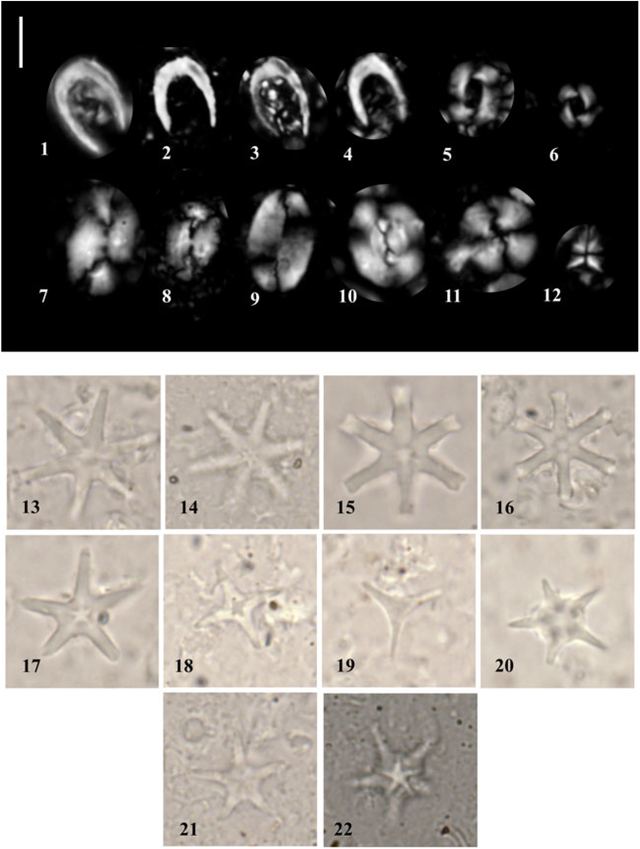
Fig. 6. Photomicrographs of selected calcareous nannofossils from Site U1457. A 5 µm scale bar is shown next to the first image. (1–4) Ceratolithus cristatus; (5) Reticulofenestra pseudoumbilicus; (6) R. pseudoumbilicus (5–7 µm); (7, 8) Helicosphaera carteri; (9) Pontosphaera japonica; (10) Reticulofenestra bisecta (reworked); (11) Calcidiscus leptoporus; (12) Sphenolithus abies; (13, 14) Discoaster brouweri; (15, 16) Discoaster surculus; (17) Discoaster asymmetricus; (18) Discoaster tamalis; (19) Discoaster triradiatus; (20) Discoaster bergenii; and (21, 22) D. berggrenii. (1–6, 8, 10, 12, 21) from U1457C-45R-4, 7 cm; (7, 9, 17, 18) from U1457C-35R-3, 32 cm; and (11, 13–16, 19, 20, 22) from U1457C-49R-2, 27 cm.
Higher-resolution sampling has allowed us to refine the position of some bioevents and add additional bioevents that were not used for construction of the shipboard age model due to their paucity in the examined samples. Positions of nannofossil datums in all holes are given in online Supplementary Tables S3 (U1456) and S4 (U1457), with those used to define the age model included in Tables 1 and 2. Top Discoaster pentaradiatus (2.39 Ma) is placed at 419.54 m CCSF, which is consistent with the revised depth of the base of G. truncatulinoides (1.93 Ma) at 400.75 m CCSF. The increased sampling resolution allowed for a more accurate placement of the top of Discoaster surculus as only sparse numbers of specimens were identified shipboard. The top of D. surculus (2.49 Ma) is identified at 423.63 m CCSF. The top of the genus Sphenolithus is recorded at 515.27 m CCSF and calibrated to 3.54 Ma.
We did not use the base of Discoaster tamalis (4.13 Ma) when constructing the shipboard age model due to its sparse presence; however, a more reliable base was identified post-cruise at 539.40 m CCSF. The top of Discoaster quinqueramus (5.59 Ma) was identified deeper at 539.40 m CCSF during post-cruise analysis, with the sporadic occurrences above considered to be reworked (online Supplementary Table S5, available at http://journals.cambridge.org/geo). Nicklithus amplificus has a relatively short range calibrated to between 6.91 and 5.94 Ma. We recorded its base at 628.94 m CCSF and its top at 610.21 m CCSF. The base Amaurolithus spp. (7.42 Ma) occurs at 644.91 m CCSF.
4.b. Palaeomagnetism
Many of the chron boundaries have been revised slightly based on post-cruise analyses, and their positions are listed in Tables 1 and 2 with the most important adjustments made in the upper Miocene section. We identified 10 magnetic polarity reversals in Site U1456 that we correlate with the geomagnetic polarity time scale (GPTS) of Gradstein et al. (Reference Gradstein, Ogg, Schmitz and Ogg2012) within the constraints provided by biostratigraphy. We also identified 11 magnetic polarity reversals for Site U1457. Based on the new results from the calcareous nannofossils, we made a significant revision to the magnetostratigraphic interpretations for these reversals at Site U1457 with the revised magnetostratigraphy used here shown in Figure 5. Details of the correlation of reversals to the GPTS are discussed in Section 5.a below. All magnetic data are available from the MagIC database.
4.c. Strontium isotope ages
Four samples analysed from Site U1457 yielded ages of 5.08–7.70 Ma (online Supplementary Figure S3; Table 2) that are in reasonably good agreement with the biostratigraphic and palaeomagnetic datums. Planktonic and benthic foraminifer specimens from Sample U1457C-47R-1, 6–10 cm (633.31 m CCSF), were measured in separate runs and yielded significantly different ages of 6.60 Ma and 6.00 Ma, respectively. Diagenetic alteration or inclusion of Sr from clay during analysis would most likely increase the measured 87Sr/86Sr and result in a younger age than expected, which could explain the difference between the benthic and planktonic foraminifer ages from the same sample. This could also explain the young age for Sample U1457C-46R-2, 100–104 cm (625.94 m CCSF).
5. Discussion
5.a. Age models
All datums used for the revised age models are compiled in Table 1 (Site U1456) and Table 2 (Site U1457). Datum label numbers given in the tables correspond to the numbers shown next to chronostratigraphic events in Figures 7 and 8. The two sites record similar sedimentation histories from the late Miocene Epoch to the present, which we divide into sediment packages (called units) that have a distinct origin (mass-transport deposit (MTD)) or are bounded by unconformities. The age and composition of the sediment recovered below the MTD is different between the two sites, with Site U1457 recording a significantly longer hiatus between deposition of the lowermost sediment package and the overlying MTD.
5.a.1. Site U1456
The section recovered at Site U1456 spans the upper Miocene to Holocene stratigraphy (units 3–6) with a short interval of lower–middle Miocene stratigraphy (unit 1) below a large MTD (unit 2) (Fig. 7; Table 1). Unit 1 is dated as early–middle Miocene age based on the presence of the calcareous nannofossil Sphenolithus heteromorphus (event 41 in Fig. 7 and Table 1) at 1111.49 m CCSF.
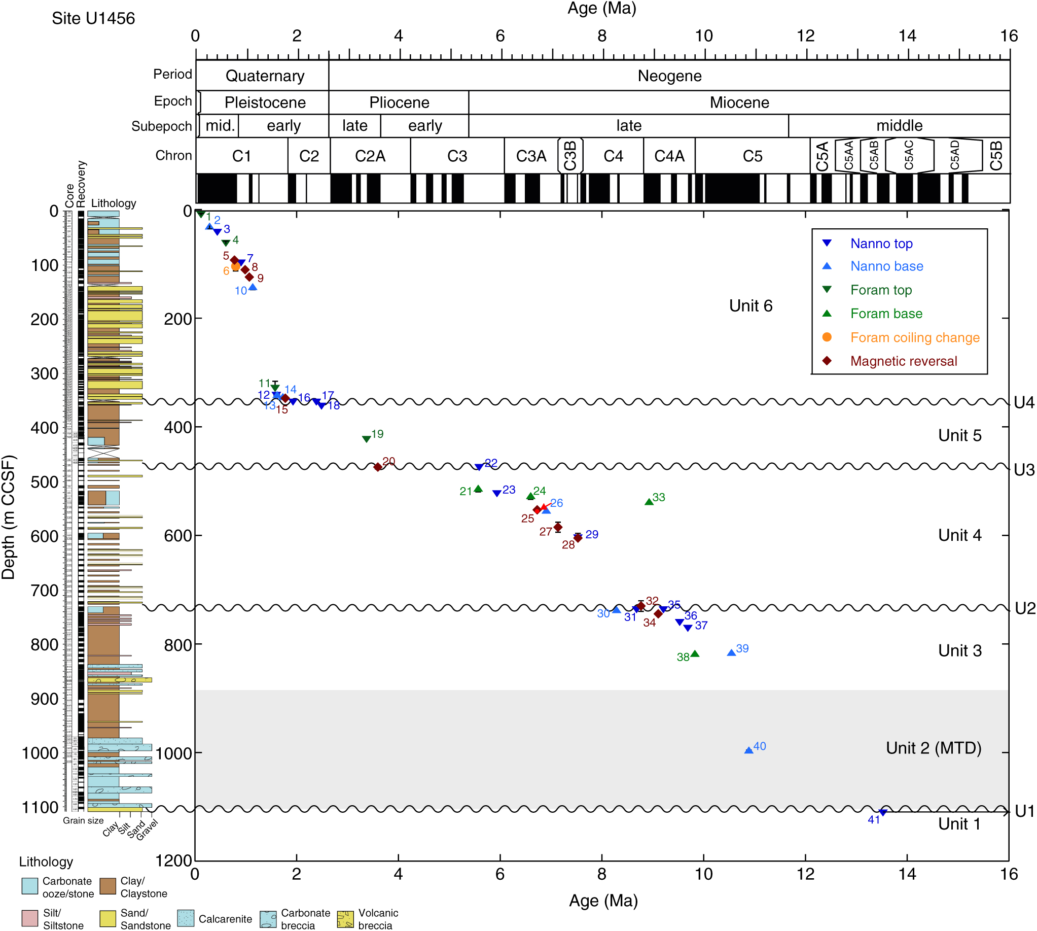
Fig. 7. Chronostratigraphic framework for Site U1456. Blue triangles are calcareous nannofossil events (up are tops, down are bases); green triangles are foraminifera events (up are tops, down are bases); orange circle is change in foraminifer coiling direction; and maroon diamonds are palaeomagnetic chron boundaries. Black lines represent error bars (both age and depth). See text (Section 5.d) for discussion of red arrow. Number represents chronostratigraphic event (refer to datum labels in Table 1).
The base of unit 2 is an unconformity (U1 on Fig. 7) defined by a distinct change in sediment composition at 1110.46 m CCSF. Unit 2 is composed of a mixture of lithologies that show a variety of sedimentary structures including microfaults, folds and inclined to vertical bedding (Pandey et al. Reference Pandey, Clift and Kulhanek2016) that indicate deposition as an MTD (identified as the Nataraja Slide; Calvès et al. Reference Calvès, Huuse, Clift and Brusset2015) and an interruption to hemipelagic and siliciclastic sedimentation at the site. The base of Catinaster coalitus (event 40) at 10.89 Ma occurs at 995.54 m CCSF and is recorded within unit 2. The top of unit 2 is intermixed with the resumption of in situ deposition, tentatively identified in Core U1456D-38R (c. 817 m CCSF), yielding a total MTD thickness of at least 295 m. The timing of the mass-transport event is constrained by the presence of C. coalitus (event 40) at 995.54 m CCSF. The presence of this taxon within the MTD indicates that the event happened sometime after the evolution of C. coalitus at 10.89 Ma.
Two biostratigraphic events at the bottom of Core U1456D-37R constrain the age of in situ deposition (unit 3) overlying the MTD to the late Miocene Epoch. The bases of the nannofossil Discoaster hamatus (10.55 Ma; event 39) and planktonic foraminifer Neogloboquadrina acostaensis (9.83 Ma; event 38) are found at 816.04 m CCSF and 817.72 m CCSF, respectively. Above this is a sequence of biostratigraphic events that includes the top of C. coalitus (9.69 Ma; event 37) at 771.58 m CCSF and the top of D. hamatus (9.53 Ma; event 36) at 760.47 m CCSF. We identify another unconformity (U2) at c. 737.47 m CCSF from a clustering of biostratigraphic events at that depth, including the tops of Discoaster bollii (9.21 Ma; event 35) and Minylitha convallis (8.68 Ma; event 31), and base of Discoaster berggrenii (8.29 Ma; event 30). This sequence of datums allows us to tie two magnetic polarity reversals above and below unconformity U2 to the GPTS (Gradstein et al. Reference Gradstein, Ogg, Schmitz and Ogg2012). The magnetic reversal (event 34) at 745.00 m CCSF in unit 3 is correlated with the top of Chron C4Ar (9.11 Ma), and the magnetic polarity reversal (event 32) at 730.28 m CCSF near the base of unit 4 is tied to the top of Chron C4An (8.77 Ma).
Above unconformity U2, the upper Miocene unit 4 consists of c. 250 m of sediment deposited between c. 8.7 and 5.6 Ma. A series of three magnetic polarity reversals (events 28, 27 and 25) are correlated with the GPTS based on several biostratigraphic datums. The top of Discoaster loeblichii (7.53 Ma; event 29) is identified at 604.68 m CCSF, which allows correlation of the magnetic reversal at 605.11 m CCSF (event 28) with the top of Chron C4n (7.53 Ma). The base of N. amplificus (6.91 Ma; event 26) at 554.01 m CCSF and the base of Pulleniatina primalis (6.60 Ma; event 24) at 527.12 m CCSF constrain the magnetic reversals at 585.21 m CCSF (event 27) and 553.04 m CCSF (event 25) to the tops of Chrons C3Bn (7.14 Ma) and C3Ar (6.73 Ma), respectively.
An interval of chalk was deposited during the late Miocene Epoch (c. 6.6–5.6 Ma), with the age constrained by the base of P. primalis (6.60 Ma; event 24) at 527.12 m CCSF, the top of N. amplificus (5.94 Ma; event 23) at 523.39 m CCSF, and the base of Globorotalia tumida (5.57 Ma; event 21) at 513.42 m CCSF. The top of D. quinqueramus (5.59 Ma; event 22) is recorded at 475.10 m CCSF, above which there is a noticeable change in the nannofossil assemblage that suggests the presence of a hiatus (U3 on Fig. 7) encompassing the Miocene–Pliocene boundary. The absences of Ceratolithus acutus (total range 5.35–5.04 Ma), Amaurolithus primus (top at 4.50 Ma) and Amaurolithus tricorniculatus (top at 3.92 Ma) in the sediment above unconformity U3 indicate an age of younger than 3.92 Ma for the base of unit 5 at c. 475 m CCSF. This allows the magnetic polarity reversal at 474.46 m CCSF (event 20) to be tied to the top of Chron C2Ar (3.596 Ma). Several biostratigraphic events constrain deposition of unit 5 to the late Pliocene – earliest Pleistocene Epochs, including the top of Sphaeroidinellopsis seminulina (3.375 Ma; event 19) at 423.47 m CCSF and the top of D. surculus (2.49 Ma; event 18) at 362.28 m CCSF. The top of unit 5 is marked by another unconformity, identified by the presence of the tops of D. pentaradiatus (2.39 Ma; event 17) and Discoaster brouweri (1.93 Ma; event 17) in the same sample at 354.63 m CCSF.
Several nannofossil datums are identified in close proximity near the base of unit 6, just above unconformity U4, including the base of Gephyrocapsa spp. > 4 µm (1.73 Ma; event 14) at 344.83 m CCSF, base of Gephyrocapsa spp. > 5.5 µm (1.62 Ma; event 13) at 341.10 m CCSF, and top of Calcidiscus macintyrei (1.60 Ma; event 12) at 342.24 m CCSF. This sequence of events allows the magnetic reversal at 347.58 m CCSF (event 15) to be correlated with the top of Chron C2n (1.778 Ma). The age of an interval of rapid sedimentation in the lower part of unit 6 is constrained by the aforementioned nannofossil datums (events 14–12), as well as the top of N. acostaensis (1.58 Ma; event 11) at 329.41 m CCSF. The next biostratigraphic event above this is the base of Reticulofenestra asanoi (1.14 Ma; event 10), identified at 146.38 m CCSF. Magnetic reversals at 124.56 m CCSF (event 9) and 111.00 m CCSF (event 8) are correlated with the tops of Subchrons C1r.2r (1.072 Ma) and C1r.1n (0.988 Ma), respectively.
The age model for sedimentation during the last c. 1 Myr at Site U1456 is well-constrained with seven biostratigraphic and magnetic reversal events (Fig. 7; Table 1). The top of R. asanoi (0.91 Ma; event 7) and the Pulleniatina coiling change to dominantly dextral forms (0.80 Ma; event 6) at 98.60 m CCSF and 104.36 m CCSF, respectively, fit well with the magnetic reversal correlated with the Matuyama–Brunhes boundary (C1r; 0.781 Ma) at 93.17 m CCSF (event 5). Other biostratigraphic events include the top of Globorotalia tosaensis (0.61 Ma; event 4) at 62.10 m CCSF, the top of Pseudoemiliania lacunosa (0.44 Ma; event 3) at 41.93 m CCSF, the base of Emiliania huxleyi (0.29 Ma; event 2) at 30.56 m CCSF, and the top of Globigerinoides ruber pink (0.12 Ma; event 1) at 9.60 m CCSF. An oxygen isotope stratigraphy for this site has also been developed for the last 1.2 Myr by Kim et al. (Reference Kim, Khim, Ikehara and Lee2018).
5.a.2. Site U1457
The succession recovered at Site U1457 is very similar to that cored at Site U1456, and consists of upper Miocene – Holocene sediments (units 3–6) separated by unconformities and overlying an upper Miocene MTD (unit 2) (Table 2; Fig. 8). Unlike at Site U1456, the sediment below the MTD (unit 1) is significantly older (early Paleocene) (Table 2) and consists of c. 30 m of marine sediment with no apparent input from the Indus Fan. The lower Paleocene section is hydrothermally altered and overlies basaltic basement (Pandey et al. Reference Pandey, Clift and Kulhanek2016). It contains an early Paleocene assemblage that includes Coccolithus pelagicus, Cruciplacolithus primus, Cruciplacolithus tenuis and Prinsius spp. The age of unit 1 is younger than 63.25 Ma based on the presence of the nannofossil Ellipsolithus macellus (event 51 on Table 2 and Fig. 8) at 1084.45 m CCSF. The absence of Fasciculithus spp. (event 50 on Table 2) further constrains the age to older than 62.13 Ma.

The top of unit 1 is marked by an abrupt lithologic change between Cores U1457C-92R and 93R (1067.35 m CCSF). The range of lithologies in unit 2 (MTD) at Site U1457 is similar to that of unit 2 at Site U1456, although the total thickness of the MTD at Site U1457 is significantly less (c. 190 m). As at Site U1456, the age of the transported deposit is constrained by the presence of C. coalitus (base at 10.89 Ma; event 49), as well as Discoaster bellus (base at 10.40 Ma; event 48), which are both present within the MTD at 1003.10 m CCSF. Another event, the base of N. acostaensis (9.83 Ma; event 47), is identified near the top of the MTD at 889.66 m CCSF, somewhat below the first downhole appearance of tilted bedding in Core U1457C-71R at c. 870 m CCSF. This event is identified just above obviously deformed bedding at Site U1456, so its presence below tilted bedding at Site U1457 may help to further constrain the timing of MTD emplacement if it was not introduced into the uppermost MTD sediments through burrowing. The presence of these taxa within the MTD provide a maximum age of 9.83 Ma (based on N. acostaensis) or 10.89 Ma (based on C. coalitus) for the timing of the event, whereas sediment in unit 3 overlying the MTD provides a minimum age of 9.69 Ma. The timing of the event is further discussed in Section 5.b below.
The resumption of background sedimentation at Site U1457 is indicated by a succession of biostratigraphic events and one palaeomagnetic reversal. The top of C. coalitus (9.69 Ma; event 45) is identified at 860.57 m CCSF and the top of D. bollii (9.21 Ma; event 44) is found at 851.06 m CCSF. These events help to correlate the magnetic polarity reversal at 865.19 m CCSF (event 46) with the top of Chron C5n. The concurrence of two nannofossil datums, the top of M. convallis (8.68 Ma; event 43) and the base of D. quinqueramus (8.12 Ma event 42), at 839.24 m CCSF indicates an unconformity (U2) at the top of unit 3.
The lower part of unit 4 (between c. 839 m and 675 m CCSF) lacks age control; however, the overlying hemipelagic succession between 675 m and 610 m CCSF is well dated with a sequence of biostratigraphic events, Sr isotope ages and magnetic polarity reversals. The revised placement of the bases of Amaurolithus spp. (7.42 Ma; event 38) and N. amplificus (6.91 Ma; event 35) are identified at 644.91 m CCSF and 628.94 m CCSF, respectively. The base of Pulleniatina primalis (6.60 Ma; event 33) is found at 618.43 m CCSF, and the top of N. amplificus (5.94 Ma; event 30) is found at 610.21 m CCSF. These biostratigraphic events help to constrain a sequence of four magnetic polarity reversals. The reversals at 675.05 m CCSF (event 41) and 663.92 m CCSF (event 39) are correlated with the tops of Chrons C4r (8.11 Ma) and C4n (7.53 Ma), respectively. The events at 643.60 m CCSF (event 36) and 624.83 m CCSF (event 32) are correlated with the tops of Subchrons C3Br.2r (7.29 Ma) and C3An.1r (6.25 Ma), respectively. Sr isotope ages from near the base of the unit (events 40 and 37) correlate well with the other chronostratigraphic tie points (Fig. 8). Events 31 and 34 are Sr isotope ages from benthic and planktonic foraminifers picked from the same sample but yielding significantly different ages, with the age from the benthic foraminifer (event 31) appearing too young. This is also the case for the Sr isotope age at 625.94 m CCSF (event 27), although both of these ages are within error (±1 Myr) of the overall line of correlation.
The top of unit 4 is marked by an unconformity (U3) that spans the Miocene–Pliocene boundary. The length of the hiatus is well constrained at this site (c. 1.5 Myr), with the identification of two nannofossil events at the same depth (539.40 m CCSF): the top of D. quinqueramus (5.59 Ma; event 28) and the base of D. tamalis (4.13 Ma; event 26). The top of Globoquadrina dehiscens (5.92 Ma; event 29) may be reworked up-section, as it is found at 519.87 m CCSF, above unconformity U3 (Fig. 8).
Unit 5 is dated to between c. 4.1 and 2.3 Ma. The tops of Sphenolithus spp. (3.54 Ma; event 24) and Dentoglobigerina altispira (3.30 Ma; event 23) are identified at 515.27 m CCSF and 485.27 m CCSF, respectively. These datums help to correlate the magnetic polarity reversal at 484.56 m CCSF (event 25) with the top of Chron C2Ar (3.596 Ma). The bases of D. surculus (2.49 Ma; event 21) and D. pentaradiatus (2.39 Ma; event 20) are found in close proximity to each other at 423.63 m CCSF and 419.54 m CCSF, respectively. These data constrain the magnetic polarity reversal at 422.16 m CCSF (event 22), allowing correlation with the top of Chron C2An (2.58 Ma).
A short unconformity (U4) marks the top of unit 5 and is identified by the concurrence of the tops of Globoturborotalita woodi (2.30 Ma; event 19) and D. brouweri (1.93 Ma; event 17) at 402.62 m CCSF. The base of G. truncatulinoides (1.93 Ma; event 16) is also found near this depth at 400.75 m CCSF. These data help to correlate the magnetic reversal at 403.02 m CCSF (event 15) with the top of Chron C2n (1.778 Ma). The age of the lower part of unit 6 is constrained by the bases of Gephyrocapsa spp. > 4 µm (1.73 Ma; event 14) and Gephyrocapsa spp. > 5.5 µm (1.62 Ma; event 13) at 388.72 m CCSF and 365.23 m CCSF, respectively. The top of the foraminifer N. acostaensis (1.58 Ma; event 12) is present at 211.64 m CCSF, although this event may be reworked up-section here, as it is found near the base of the sequence at Site U1456 (event 11 in Fig. 7).
A series of biostratigraphic events and magnetic polarity reversals constrains the age model for the top 95.69 m CCSF of the site. The tops of Globoturborotalita obliquus (1.30 Ma; event 11) and Gephyrocapsa spp. > 5.5 µm (1.24 Ma; event 10) and the base of R. asanoi (1.14 Ma; event 9) are identified at 95.69 m CCSF, 89.33 m CCSF and 80.04 m CCSF, respectively. These events help to correlate magnetic polarity reversals at 76.20 m CCSF (event 8) and 66.98 m CCSF (event 7) with the tops of Subchrons C1r.2r (1.072 Ma) and C1r.1n (0.988 Ma), respectively. The tops of R. asanoi (0.91 Ma; event 6) and G. tosaensis (0.61 Ma; event 4) at 54.86 m CCSF and 31.53 m CCSF, respectively, constrain the magnetic polarity reversal at 47.15 m CCSF to the Matuyama–Brunhes boundary (top of Chron C1r; 0.781 Ma). The remainder of the stratigraphy is constrained by the top of Pseudoemiliania lacunosa (0.44 Ma; event 3) at 21.47 m CCSF, the base of Emiliania huxleyi (0.29 Ma; event 2) at 25.87 m CCSF, and the top of Globigerinoides ruber pink (0.12 Ma; event 1) at 3.70 m CCSF. We note that the sequence of events for P. lacunosa and E. huxleyi appear to be reversed; however, this is likely due to uncertainty from only looking at samples every c. 10 m, as well as the difficulty of identifying the base of E. huxleyi using a transmitted light microscope instead of a scanning electron microscope.
5.b. Sedimentary succession
The sedimentary successions are similar at the two sites, with four units of sediment (units 3–6) overlying an MTD (unit 2). Emplacement of the MTD eroded different amounts of sediment at each site, as indicated by the very different ages of sediment underlying the MTD: early–middle Miocene (13.53–17.71 Ma) at Site U1456 and early Paleocene (62.13–63.25 Ma) at Site U1457. The sedimentary sequence at Site U1456 is thicker (estimated at c. 1490 m based on seismic reflection profiles) as the site is located in the middle of the Laxmi Basin (Fig. 2), whereas Site U1457 is located on the flank of Laxmi Ridge and has only c. 1090 m of sedimentary fill overlying the basaltic basement (Pandey et al. Reference Pandey, Clift and Kulhanek2016). At Site U1457, much of the Cenozoic sediments that were emplaced were removed by the MTD and only c. 30 m of lower Paleocene marine sediment that lacks Indus-derived material (unit 1 on Fig. 8) remains between the base of the MTD and basement. With a significantly thicker sedimentary succession at Site U1456, the MTD removed only Miocene-aged material, with upper-lower–middle Miocene sediment present below the MTD. At Site U1456, the Miocene sediment in unit 1 is composed of interbedded grey silty claystone and silty sandstone, and likely represents a mixture of Indus Fan and hemipelagic deposition (Pandey et al. Reference Pandey, Clift and Kulhanek2016).
The MTD (unit 2) varies in thickness from c. 300 m at Site U1456 to c. 190 m at Site U1457. The MTD is dominated by calcarenite, calcilutite, breccia and limestone that show deformation structures throughout the deposit including microfaults, tilted bedding and slickensides (Pandey et al. Reference Pandey, Clift and Kulhanek2016). Clasts of vesicular volcanic rock may derive from Deccan Plateau basalt and some of the limestone indicates deposition in shallow water, suggesting that the MTD is of shelf origin (Pandey et al. Reference Pandey, Clift and Kulhanek2016). Calvès et al. (Reference Calvès, Huuse, Clift and Brusset2015) identified a potential source area for the MTD on the West India continental margin offshore of the Saurashtra platform using seismic profiles and bathymetric maps. They named the MTD the Nataraja Slide and estimated a total volume of c. 19 × 103 km3, making it the second-largest known submarine landslide. Shipboard biostratigraphy indicates that much of the sediment within the MTD is of Palaeogene age, although there are intervals that also contain early–middle Miocene taxa (Pandey et al. Reference Pandey, Clift and Kulhanek2016). The presence of the nannofossil C. coalitus (total range 10.89–9.69 Ma) within the MTD at both sites constrains the timing of emplacement, which must have happened after the origination of C. coalitus at 10.89 Ma. Furthermore, the planktonic foraminifer N. acostaensis (base at 9.83 Ma) is found in sediment immediately above obviously deformed strata at Site U1456 and just below obviously deformed strata at Site U1457, suggesting that the event occurred after 9.83 Ma. At both sites, C. coalitus is present in undeformed sediment above the MTD. While we cannot completely rule out reworking, we interpret that emplacement happened before the extinction of C. coalitus at 9.69 Ma, providing a narrow interval between c. 9.83 and 9.69 Ma for MTD emplacement. The age of this event also constrains the length of the hiatus in unconformity U1 to 3.8–8.0 Myr at Site U1456 and c. 52.5–53.5 Myr at Site U1457.
At both sites, sediment above the MTD (unit 3) is primarily mudstone with sparse interbedded, graded sand beds that are interpreted as distal turbidites (Pandey et al. Reference Pandey, Clift and Kulhanek2016). A similar sequence of biostratigraphic events is found in unit 3 at both sites, indicating a late Miocene age. The sedimentation rate in unit 3 is higher at Site U1456 (10 cm/kyr) compared with Site U1457 (c. 6 cm/kyr). Unit 3 is separated from the overlying unit 4 by a disconformity (U2 on Figs 7, 8) in the upper Miocene sediments, constrained to 9.21–8.12 Ma. At Site U1456, the hiatus is identified by the tops of M. convallis (8.68 Ma) and D. bollii (9.21 Ma), as well as the base of D. berggrenii (8.29 Ma) at the same horizon, indicating a hiatus of at least 0.9 Myr. The last occurrence of D. bollii is found slightly deeper than the last occurrence of M. convallis at Site U1457 (851.06 m CCSF and 839.24 m CCSF, respectively), which suggests deposition continued at this site slightly longer after 9.21 Ma relative to Site U1456. At Site U1457, the top of D. quinqueramus (8.12 Ma) is found at the same horizon as M. convallis (top at 8.68 Ma), indicating a hiatus of at least 0.56 Myr.
Unit 4 is also dominated by mudstone; however, thin sand beds are more frequent and intervals of hemipelagic chalk are also present in the upper part of unit 4 at both sites. The terrigenous sediment is interpreted as distal turbidity current deposits, with similar sedimentation rates at both sites (c. 9–10 cm/kyr). Siliciclastic-dominated deposition was interrupted during the late Miocene Epoch by deposition of hemipelagic chalk at c. 8–6 Ma, which correlates with a climate transition marked by a change from C3- to C4-dominated terrestrial vegetation in the region (e.g. Quade et al. Reference Quade, Cerling and Bowman1989; Cerling et al. Reference Cerling, Harris, MacFadden, Leakey, Quade, Eisenmann and Ehieringer1997; Strömberg, Reference Strömberg2011). Resumption of siliciclastic input occurred at c. 6 Ma at both sites, with renewed deposition of sand and mud.
A hiatus of c. 1.4–1.6 Myr that spans the Miocene–Pliocene boundary (U3 on Figs 7, 8) separates unit 4 from unit 5 at both sites. At Site U1457, the presence of D. quinqueramus (top at 5.59 Ma) and D. tamalis (base at 4.13 Ma) at the same horizon (539.40 m CCSF) indicates a minimum hiatus duration of 1.46 Myr. The disconformity is better constrained at Site U1457 than at Site U1456, where D. tamalis was not identified. Sediment in unit 5 is similar to that of unit 4 and is dominantly siliciclastic, albeit with thin intervals of hemipelagic chalk. Sediment appears to be somewhat coarser-grained at Site U1457 relative to Site U1456 (Pandey et al. Reference Pandey, Clift and Kulhanek2016), although poor recovery at Site U1457 prevented this observation from being quantified. Sedimentation rates were similar at the two sites, at c. 8–10 cm/kyr.
Another short hiatus (unconformity U4) separates unit 5 from unit 6 and encompasses part of the early Pleistocene Epoch. It is identified by the tops of D. brouweri (1.93 Ma) and D. pentaradiatus (2.39 Ma) at the same horizon (354.63 m CCSF) at Site U1456. At Site U1457, the hiatus appears to be of slightly shorter duration and is indicated by the tops of Globoturborotalita woodi (2.3 Ma) and D. brouweri (1.93 Ma) at the same horizon (402.62 m CCSF). Furthermore, the last occurrence of D. brouweri occurs within a normal polarity zone at both Sites U1456 and U1457, whereas its extinction at 1.93 Ma is correlated with a reversed polarity interval at the top of Chron C2r (Gradstein et al. Reference Gradstein, Ogg, Schmitz and Ogg2012). Taken together, these lines of evidence suggest a hiatus of c. 0.45 Myr duration during the early Pleistocene Epoch.
The lower part of unit 6 consists of a thick section (> 200 m) of siliciclastic sediment deposited very rapidly during the early Pleistocene Epoch. This sediment is very coarse-grained at Site U1456. Recovery of this interval at Site U1457 was much poorer due to use of the rotary core barrel coring assembly, so it is difficult to determine the dominant grain size. Regardless, sedimentation rates over this interval were at least 40 cm/kyr at Site U1456 and 60 cm/kyr at Site U1457. These deposits are interpreted as a sheet-type lobe in a middle or lower fan setting (Pandey et al. Reference Pandey, Clift and Kulhanek2016). Sedimentation at both sites since c. 1.2 Ma was dominantly hemipelagic, with the sediment comprising deep-sea calcareous ooze interbedded with clay, silt and sand, where the sand layers comprise thin turbidite sequences likely deposited in a distal basin setting (Pandey et al. Reference Pandey, Clift and Kulhanek2016).
5.c. Regional comparison
Previous drilling in the Arabian Sea during Deep Sea Drilling Project (DSDP) Leg 23 and Ocean Drilling Program (ODP) Leg 117 (Fig. 1) provided age control for distal Indus Fan sediments. At Site 219 on the Laccadive Ridge and Site 223 on the Murray Ridge to the SE and west of our drill sites, respectively, the oldest sediment recovered was late Paleocene in age (Whitmarsh et al. Reference Whitmarsh, Weser, Ali, Boudreaux, Fleisher, Jipa, Kidd, Mallik, Matter, Nigrini, Siddiquie, Stoffers, Hamilton and Hunziker1974). This cross-basin comparison aligns with sediments at Site U1457, where a c. 30 m thick section of lower Paleocene sediment was recovered directly below the MTD and overlying the basaltic basement (Pandey et al. Reference Pandey, Clift and Kulhanek2016).
Comparison of biostratigraphic events across the Arabian Sea from the Laxmi Basin to the western-most edge of the Indus Fan indicates the rarity or absence of several Miocene nannofossil biomarkers including the genera Amaurolithus and Ceratolithus, as well as a few species of Discoaster (e.g. D. surculus, D. asymmetricus and D. tamalis) at both Sites U1456 and U1457 as well as at Sites 721, 722 and 731 (Prell et al. Reference Prell, Niitsuma, Emeis, Al-Sulaiman, Al-Tobbah, Anderson, Barnes, Bilak, Bloemendal, Bray, Busch, Clemens, de Menocal, Krissek, Kroon, Murray, Nigrini, Pedersen, Ricken, Shimmield, Spaulding, Takayama, ten Haven, Lo and Weedon1989). Genera belonging to the family Ceratolithaceae (e.g. Amaurolithus and Ceratolithus) are considered to be warm-water, open-ocean dwellers (Wade & Bown, Reference Wade and Bown2006) but are noticeably rare to absent in the Arabian Sea. This scarcity in the fan setting might be a result of dilution due to high rates of terrigenous sediment input or, in the wider Arabian Sea, by exclusion from higher-productivity environments.
The hiatus encompassing the Miocene–Pliocene boundary at Sites U1456 and U1457 is recorded at several other sites within the Arabian Sea, from the southern-most and western-most edge of the Indus Fan (DSDP Sites 221 and 224 and ODP Sites 720, 721 and 722 and possibly Site 731). Other sites drilled in the Arabian Sea (including DSDP Sites 219, 220, 222 and 223) recovered the Miocene–Pliocene boundary.
5.d. Taxonomy and age calibrations
The family Ceratolithaceae includes the distinctive and biostratigraphically important Neogene genera Amaurolithus, Ceratolithus, Nicklithus, Orthorhabdus and Triquetrorhabdulus. The ornate nannolith genera Amaurolithus, Ceratolithus and Nicklithus are useful late Miocene – Pliocene biostratigraphic markers for low-latitude, open-ocean settings.
Amaurolithus primus is the first representative of the genus Amaurolithus, which evolved from Triquetrorhabdulus rugosus during the late Miocene Epoch (Raffi et al. Reference Raffi, Backman and Rio1998). This event is dated to 7.42 Ma in the eastern Mediterranean using astronomical tuning (Raffi et al. Reference Raffi, Mozzato, Fornaciari, Hilgen and Rio2003), but is known to occur slightly later (7.36 Ma) in the Atlantic at ODP Sites 925 and 926 (Backman & Raffi, Reference Backman and Raffi1997; Shackleton & Crowhurst, Reference Shackleton, Crowhurst, Shackleton, Curry, Richter and Bralower1997). In the eastern equatorial Pacific (ODP Leg 138), the base of Amaurolithus was dated to c. 7.25 Ma at Site 844 (Shackleton et al. Reference Shackleton, Baldauf, Flores, Iwai, Moore, Raffi, Vincent, Pisias, Mayer, Janecek, Palmer-Julson and van Andel1995). The position of this event falls within the middle of Subchron C3Br.2r based on the magnetostratigraphy of Schneider (Reference Schneider, Pisias, Mayer, Janecek, Palmer-Julson and van Andel1995), equivalent to c. 7.3 Ma on the GPTS2012. At ODP Site 710 in the equatorial Indian Ocean, this event falls within Subchron C3.Br.1r (Rio et al. Reference Rio, Fornaciari, Raffi, Duncan, Backman and Peterson1990), which is equivalent to c. 7.23 Ma on the GPTS2012. The first appearance of this genus is therefore diachronous between the Mediterranean, South Atlantic, Pacific and Indian oceans, and is closer to 7.3 or 7.2 Ma in the Indian Ocean. While we plot the age as 7.42 Ma in Figure 8 (as given in GPTS2012), we suggest that this event occurs 100 or 200 kyr later at this site, which better aligns with the magnetostratigraphic interpretation for polarity reversal events above and below this datum (see red circle and arrow for event 38 in Fig. 8).
The genus Nicklithus was once included within Amaurolithus; however, phylogenetic evidence presented by Raffi et al. (Reference Raffi, Backman and Rio1998) suggested that it evolved independently and proposed a new genus. Both the evolution and extinction of N. amplificus are stratigraphically significant bioevents in the late Miocene Epoch (range reported as 6.91–5.94 Ma in Gradstein et al. Reference Gradstein, Ogg, Schmitz and Ogg2012). The evolution of N. amplificus is astronomically tuned at 6.91 Ma in the South Atlantic at ODP Sites 925 and 926 (Backman & Raffi, Reference Backman and Raffi1997; Shackleton & Crowhurst, Reference Shackleton, Crowhurst, Shackleton, Curry, Richter and Bralower1997). Its first appearance is known to occur later in the eastern Mediterranean (6.68 Ma; Raffi et al. Reference Raffi, Mozzato, Fornaciari, Hilgen and Rio2003). Raffi et al. (Reference Raffi, Rio, D’Atri, Fornaciari, Rocchetti, Pisias, Mayer, Janecek, Palmer-Julson and van Andel1995) examined the occurrences of Miocene bioevents in the equatorial Indian (ODP Leg 115) and Pacific (ODP Leg 138) oceans. They reported that the first occurrence of N. amplificus occurs very near the Chron C3Ar/C3An boundary (c. 6.73 Ma) at sites in both oceans, including Sites 844 and 845 (Raffi & Flores, Reference Raffi, Flores, Pisias, Mayer, Janecek, Palmer-Julson and van Andel1995; Schneider, Reference Schneider, Pisias, Mayer, Janecek, Palmer-Julson and van Andel1995) and Site 710 (Rio et al. Reference Rio, Fornaciari, Raffi, Duncan, Backman and Peterson1990). At Site U1456, the base of N. amplificus is found within 1 m of a magnetic polarity reversal; we interpret this as the top of Chron C3Ar (6.73 Ma), supporting the younger age of c. 6.7 Ma for the evolution of N. amplificus in the Indian Ocean (see red circle and arrow for event 26 in Fig. 7 and event 35 in Fig. 8).
5.e. Microfossil reworking
The abundance of reworked Cretaceous and Palaeogene calcareous nannofossils recorded throughout the stratigraphy at Sites U1456 and U1457 were similarly recorded at Sites 222 and 731 in the western Arabian Sea (Whitmarsh et al. Reference Whitmarsh, Weser, Ali, Boudreaux, Fleisher, Jipa, Kidd, Mallik, Matter, Nigrini, Siddiquie, Stoffers, Hamilton and Hunziker1974; Prell et al. Reference Prell, Niitsuma, Emeis, Al-Sulaiman, Al-Tobbah, Anderson, Barnes, Bilak, Bloemendal, Bray, Busch, Clemens, de Menocal, Krissek, Kroon, Murray, Nigrini, Pedersen, Ricken, Shimmield, Spaulding, Takayama, ten Haven, Lo and Weedon1989). Reworked forms appear to have undergone significant diagenesis as well as dissolution and breakage, likely because of the distance travelled post-deposition. The source of the Cretaceous reworking is not immediately clear, but could originate from Cretaceous limestone outcrops in Western Pakistan and/or eroded from the Himalaya and transported by the Indus River into the fan sediments (Whitmarsh et al. Reference Whitmarsh, Weser, Ali, Boudreaux, Fleisher, Jipa, Kidd, Mallik, Matter, Nigrini, Siddiquie, Stoffers, Hamilton and Hunziker1974).
6. Conclusions
IODP Expedition 355 to the Arabian Sea cored Sites U1456 and U1457 in the Laxmi Basin. The integration of new and shipboard biostratigraphic, palaeomagnetic and geochemical data has allowed us to revise the age models, which are critical to examining the relationship between Himalayan uplift, erosion and climate during the Cenozoic Era. The stratigraphy is similar at the two sites, and includes four units of Neogene and Quaternary sediment separated by unconformities that overlay an MTD emplaced during the late Miocene Epoch. Below the MTD, the age and composition of the sediments are very different between the two sites.
Unit 1 underlies the MTD. At Site U1456, unit 1 consists of a mixture of terrigenous (likely sourced from the Indus River) and hemipelagic sediment of early–middle Miocene age. At Site U1457, unit 1 is of early Paleocene age and consists of 30 m of hydrothermally altered marine mud that directly overlies the basaltic basement.
Unit 2 is the MTD that is composed of a wide variety of mixed lithologies, including calcilutite, calcarenite, limestone and mudstone with a variety of deformation features consistent with emplacement during a mass-transport event. Biostratigraphy indicates that the MTD was emplaced between c. 9.83 and 9.69 Ma.
Unit 3 represents a return to in situ deposition above the MTD and is composed of nannofossil-rich mudstone with thin graded sandstone beds, interpreted as turbidites of the Indus Fan. The sedimentation rate for unit 3 was c. 10 cm/kyr at Site U1456 and c. 6 cm/kyr at Site U1457. The top of this unit is marked by a hiatus (unconformity U2) at both sites between c. 9.21 and 8.12 Ma.
Unit 4 includes a sequence of interbedded coarser-grained sand and mud deposited at c. 9–10 cm/kyr. Turbidite deposition was interrupted between c. 8 and 6 Ma (late Miocene) by hemipelagic chalk deposition. Turbidite deposition resumed during the late Miocene Epoch at c. 6 Ma, with sedimentation rates again c. 10 cm/kyr. The top of unit 3 is a longer hiatus (1.4–1.6 Myr) that encompasses the Miocene–Pliocene boundary.
Turbidite deposition continued in unit 5 at a rate of c. 8–10 cm/kyr. This unit was deposited between c. 4.1 and 2.4 Ma. The top of unit 5 is a short (c. 0.45 Myr) hiatus in the lower Pleistocene stratigraphy.
Unit 6 consists of a thick (c. 200 m) sequence of coarse-grained sediment deposited very rapidly (c. 40–45 cm/kyr at Site U1456 and c. 60 cm/kyr at Site U1457) between c. 1.9 and 1.2 Ma. Hemipelagic deposition has dominated the region since c. 1.2 Ma. Sedimentation rates were still high (c. 7–12 cm/kyr), but much slower than deposition during the early Pleistocene Epoch.
These revised age models will enable tighter constraint of tectonic and climate interaction as a result of Himalayan uplift.
Supplementary material
To view supplementary material for this article, please visit https://doi.org/10.1017/S0016756819000104.
Author ORCIDs
Denise K. Kulhanek, 0000-0002-2156-6383; Arun D. Singh, 0000-0003-1287-8067; Rajeev Saraswat, 0000-0003-2110-2578
Acknowledgements
This research used samples and data provided by the International Ocean Discovery Program. We thank the operational and technical staff as well as the shipboard science party for an enjoyable and successful expedition. We also thank Paul Bown, who provided suggestions for an earlier version of this manuscript, and the anonymous reviewers and editor Peter Clift for useful comments that improved this manuscript. This work was partially supported by the US Science Support Program (USSSP) National Science Foundation (NSF) award OCE1450528 funding to Lamont Doherty Earth Observatory/Columbia University (CMR, DKK, LT) and NSF Grant EAR1547263 (LT).
Declaration of interest
The authors have no conflicts of interest to declare.


