


1. Introduction
Ushered in with Wegener's (Reference Wegener1912) hypothesis of continental drift was a simple yet profound concept that later found its way into early conceptions of mantle convection by Holmes (Reference Holmes1931) before ultimately emerging as a central tenet in the theory of plate tectonics: global-scale mobilism. In the form of Wegener's continental drift, mobilism already provided a wealth of new insights; explaining, for example, the spatio-temporal distribution of faunas and facies through the shifting position of continents rather than the raising and sinking of land bridges or the total restructuring of climatic belts. But Wegener's hypothesis was hampered by the lack of a driving mechanism; what could move continents? Holmes’ (Reference Holmes1931) pioneering ideas on mantle convection provided early clues, but ones not fully appreciated or broadly adopted before the recognition of seafloor spreading (Dietz, Reference Dietz1961; Hess, Reference Hess, Engel, James and Leonard1962; Vine & Matthews, Reference Vine and Matthews1963) and the ensuing formulation of plate tectonics (Wilson, Reference Wilson1965; McKenzie & Parker, Reference McKenzie and Parker1967; Le Pichon, Reference Le Pichon1968; Morgan, Reference Morgan1968). But plate tectonics did far more than supply continental drift with a means, rather it recast Wegener's mobilistic ideas into a more fundamental mould, one in which the entire surface of Earth was at play, together with the mantle beneath it.
The development of plate tectonics in the 1960s was as transformative to the Earth sciences as Darwin's theory of evolution had been to the life sciences a century before, and it would be difficult to overstate its impact on our discipline. Through plate tectonics it has been possible to understand the process of mountain building (Dewey & Bird, Reference Dewey and Bird1970; Dewey & Burke, Reference Dewey and Burke1973; Molnar & Tapponnier, Reference Molnar and Tapponnier1975), the formation of ophiolites and accretionary complexes (Gass, Reference Gass1968; Matsuda & Uyeda, Reference Matsuda and Uyeda1971; Moores, Reference Moores1982; Cawood et al. Reference Cawood, Kröner, Collins, Kusky, Mooney and Windley2009; Dilek & Furnes, Reference Dilek and Furnes2011), the distribution of earthquakes and magmatic arcs (Isacks, Oliver & Sykes, Reference Isacks, Oliver and Sykes1968; Dickinson, Reference Dickinson1970; Ringwood, Reference Ringwood1974; Davies & Stevenson, Reference Davies and Stevenson1992; Grove et al. Reference Grove, Till, Lev, Chatterjee and Médard2009), and the nature of high and ultrahigh pressure (HP-UHP) metamorphic belts (Ernst, Reference Ernst1971; Miyashiro, Reference Miyashiro1972; Chopin, Reference Chopin2003; Ernst & Liou, Reference Ernst and Liou2008), among many other phenomena. And this new paradigm brought with it something else important: kinematic rules. By extending simple logic about how rigid caps could move about the surface of a sphere, the motion of plates could be used to predict the formation of particular boundaries, and so too could the occurrence of particular boundaries be used to infer the past motion of plates. This being immediately recognized, the early days of the plate tectonic revolution were marked by intense activity and fast-paced discovery, such that the major boundaries of the present-day plates and their recent motions were basically established within a few years (Chase, Reference Chase1972, Reference Chase1978; Minster et al. Reference Minster, Jordan, Molnar and Haines1974; Minster & Jordan, Reference Minster and Jordan1978).
In the decades that have followed, important progress and new discoveries have been achieved through the application of those plate tectonic rules to the past, in the Cenozoic and late Mesozoic. Marine magnetic anomalies and fracture zone geometries in the oceanic crust present an exquisite record of the position and orientation of fossil plate boundaries, and provide a means to directly infer the ancient relative motions between plates (Cox & Hart, Reference Cox and Hart1986). By utilizing such information, it has been possible to construct global relative plate motion models for the last ~200 Ma, which together with information from hotspot tracks can be placed into a mantle-based, or ‘absolute’, reference frame (Müller, Royer & Lawver, Reference Müller, Royer and Lawver1993; Steinberger, Sutherland & O'Connell, Reference Steinberger, Sutherland and O'connell2004; O'Neill, Müller & Steinberger, Reference O'Neill, Müller and Steinberger2005; Torsvik et al. Reference Torsvik, Müller, Van der Voo, Steinberger and Gaina2008; Doubrovine, Steinberger & Torsvik, Reference Doubrovine, Steinberger and Torsvik2012; Seton et al. Reference Seton, Müller, Zahirovic, Gaina, Torsvik, Shephard, Talsma, Gurnis, Turner and Maus2012). Such reconstructions have provided a wealth of insights, both in the pursuit of disentangling the geologic history of the surface, but also in understanding the co-evolution and interplay between the lithosphere and the mantle beneath it. The latter prospect is particularly noteworthy because the mantle – physically inaccessible and convecting – effectively veils its history.
But why stop at ~200 Ma? The plate tectonic revolution also brought with it the recognition that large-scale mobilism did not start with Pangaea; J. Tuzo Wilson realized already in 1966 that the North Atlantic basin had been preceded by an earlier ocean (later named Iapetus (Harland & Gayer, Reference Harland and Gayer1972)), introducing the concept of ‘Wilson Cycles’ (Wilson, Reference Wilson1966). The question of when modern-style plate tectonics began remains contentious, but it was certainly operating by the Neoproterozoic (~1 Ga), from which time there are unambiguous ophiolite relics and HP-UHP metamorphic assemblages (Stern, Reference Stern2005). A multitude of ‘global’ palaeogeographic reconstructions have been published for times between 1 Ga and 200 Ma (Scotese et al. Reference Scotese, Bambach, Barton, Van der Voo and Ziegler1979; Scotese & McKerrow, Reference Scotese, McKerrow, McKerrow and Scotese1990; Dalziel, Reference Dalziel1997; Meert & Van der Voo, Reference Meert and Van der Voo1997; Cocks & Torsvik, Reference Cocks and Torsvik2002; Golonka, Reference Golonka, Kiessling, Flugel and Golonka2002; Meert & Torsvik, Reference Meert and Torsvik2003; Pisarevsky et al. Reference Pisarevsky, Wingate, Powell, Johnson, Evans, Yoshida, Windley and Dasgupta2003; Torsvik & Cocks, Reference Torsvik and Cocks2004; Li et al. Reference Li, Bogdanova, Collins, Davidson, De Waele, Ernst, Fitzsimons, Fuck, Gladkochub and Jacobs2008; Domeier, Van der Voo & Torsvik, Reference Domeier, Van der Voo and Torsvik2012; Torsvik et al. Reference Torsvik, Van der Voo, Preeden, Mac Niocaill, Steinberger, Doubrovine, van Hinsbergen, Domeier, Gaina and Tohver2012, among many others), but these models have been near-exclusively built from considerations of only the positions of the continents; i.e. without explicit regard for the movement of complete (‘full’) tectonic plates. In a way, ironically, these models represent a return to Wegener's paradigm of continental drift – and as such forgo many of the powerful insights and advancements afforded by plate tectonics. The reason for this is simple: owing to the relentless operation of subduction, virtually all in situ oceanic crust older than 200 Ma has been recycled, and with it the marine magnetic anomalies, fracture zones and hotspot tracks that documented the pre-200 Ma kinematics of ~70% of the Earth's surface (Fig. 1).
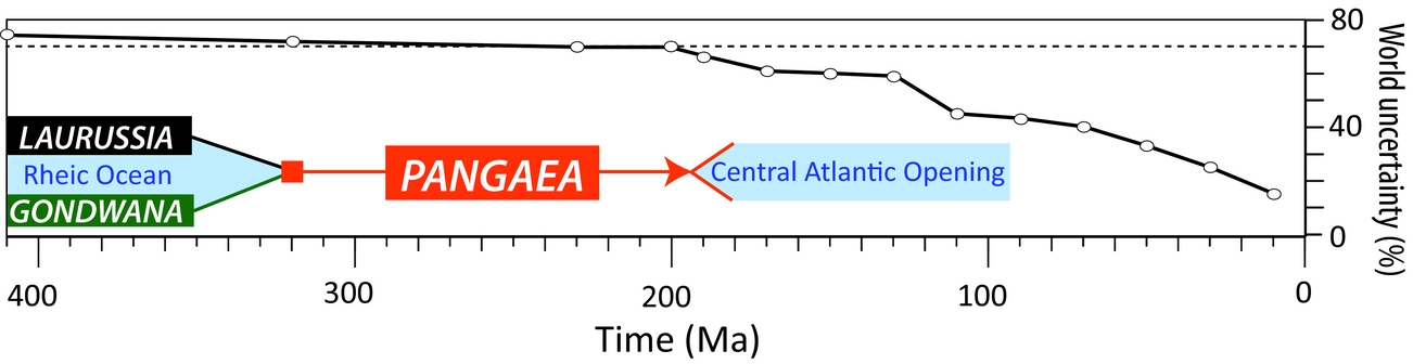
Figure 1. World uncertainty back to 410 Ma. The ‘world uncertainty’ is the fraction of the global surface area that is missing at any given time – mostly owing to the loss of oceanic lithosphere by subduction – and will therefore be a synthetic estimation in any given plate model. The flattening of the curve at ~200 Ma occurs because oceanic lithosphere is near-entirely lost by that time and the remaining ~30% of the surface is continental lithosphere. The late Palaeozoic was dominated by the great continent of Gondwana and Laurussia (Baltica, Avalonia and Laurentia) which collided at ~320 Ma to form the supercontinent Pangaea. The break-up of Pangaea corresponded with the opening of the Central Atlantic and formation of the bulk of the earliest in situ oceanic crust still preserved today.
The task of constructing a pre-Jurassic plate tectonic model is thus challenging, but the motivations for trying are compelling. Geodynamic simulations and tomographic–palaeogeographic correlations suggest that mantle overturn occurs on a timescale of ~150–200Ma (Bunge et al. Reference Bunge, Richards, Lithgow-Bertelloni, Baumgardner, Grand and Romanowicz1998; Steinberger, Torsvik & Becker, Reference Steinberger, Torsvik and Becker2012; Domeier et al. Reference Domeier, Doubrovine, Torsvik, Spakman and Bull2016), meaning that coupling of Mesozoic–Cenozoic plate models with numerical mantle simulations will only yield information about the most recent mantle convection cycle. To investigate longer-term changes in mantle convection, longer-term plate models are needed. Such investigations would also be useful in furthering present debates about the nature, stability and longevity of the large low shear velocity provinces (LLSVP) in the lowermost mantle (Bull, Domeier & Torsvik, Reference Bull, Domeier and Torsvik2014; Zhong & Rudolph, Reference Zhong and Rudolph2015; Flament et al. Reference Flament, Williams, Müller, Gurnis and Bower2017; Torsvik & Domeier, Reference Zhong and Rudolph2017). Pre-Jurassic plate models also open new possibilities for palaeoclimate modelling, allowing simulations to be run with global palaeogeography and synthetic bathymetry, and enabling quantification of and direct comparison with a host of climatically-important, global-scale processes (seafloor production rate, subduction flux, volcanic arc length, etc.) (Vérard et al. Reference Vérard, Hochard, Baumgartner, Stampfli and Liu2015). Global plate models, being inherently seamless in space and time, also wield predictive power, allowing new and testable hypotheses to be formulated from the model itself, which can be evaluated against new observations.
In this paper we present tools, methods and a workflow that can be used to construct pre-Jurassic full-plate models. ‘Full-plate models’ (hereafter just ‘plate models’) require the explicit definition and management of the entire breadth of lithospheric plates, i.e. including both continental and oceanic components. A ‘global’ plate model is therefore completely globally defined, meaning that all points on the surface are registered to a plate at any given time. The constituent plates of the model are moreover required to evolve continuously in time and in accordance with plate tectonic expectations. In the following sections we discuss tools and methods with specific reference to the reconstruction software GPlates (www.gplates.org), but the concepts presented are general and thus applicable to any other reconstruction software.
2. Basic tools
2.a. Euler poles and reconstruction networks
The fundamental mathematical tool of plate tectonics, as demonstrated by McKenzie & Parker (Reference McKenzie and Parker1967) and Morgan (Reference Morgan1968), is Euler's rotation theorem, from which it can be shown that any displacement of a rigid body across the surface of a sphere can be represented by a rotation about an axis which passes through the centre of the sphere (Fig. 2). So long as the plates are assumed to be rigid, all their various motions can therefore be neatly and concisely catalogued as a series of poles paired with angular displacements. In the general case, the reconstruction of a given plate can be defined by a rotation with respect to another plate (or otherwise mobile reference), and so in practice it is necessary to also document the identity of this reference. Most plate reconstruction algorithms (including that in GPlates) operate from rotation files built simply from this information, as in the following:
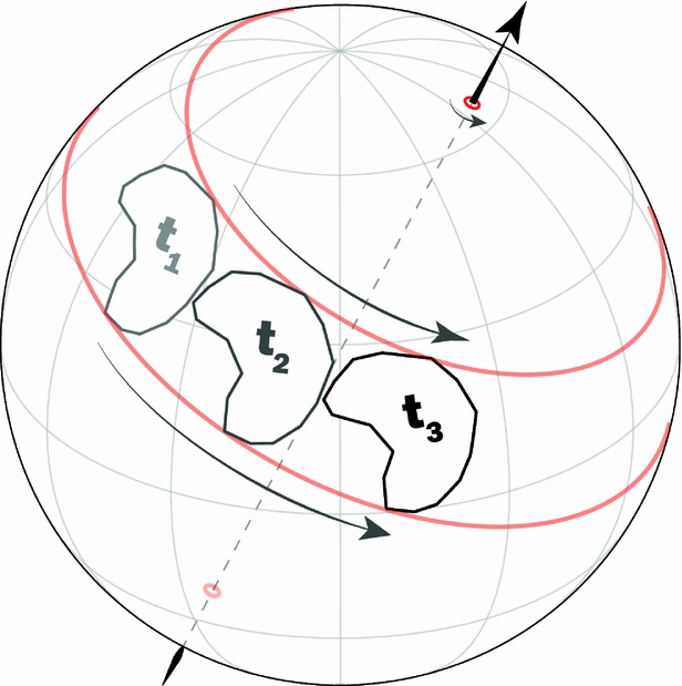
Figure 2. Motion on a sphere defined by rotation about an Euler pole. The continent's motion from time t 1 to t 3 can be represented by a rotation about an axis that passes through the centre of the sphere, as shown. To avoid ambiguity, the motion is specifically described with respect to one of the two poles of that axis (where the axis intersects the spherical surface), a so-called ‘Euler pole’. By convention, a positive rotation is anticlockwise about an Euler pole, as depicted here. The motion depicted could be equivalently described by a negative rotation of the same magnitude about the antipodal Euler pole.

In rotation models where plate motions are regularly referenced to other plates, the reconstruction is said to be networked, and often these reconstruction networks are hierarchical, resembling a branching tree (Fig. 3). This is almost invariably the structure of Cenozoic to late Mesozoic plate models because they are most commonly founded on marine geophysical records which preserve information about relative, rather than absolute, plate motions. In a global model of such relative motions, one plate is elected to be the ‘anchor’ plate, which, in the reference frame of the relative motion model, is stationary – and this anchor plate also typically acts as the ‘root’ of the reconstruction tree. The restoration of that anchor plate to its appropriate position in an absolute reference frame (according to palaeomagnetic or hotspot track data, for example), would thus result in the passive restoration of all other elements of the plate model to their appropriate absolute positions (Torsvik et al. Reference Torsvik, Müller, Van der Voo, Steinberger and Gaina2008).

Figure 3. Reconstruction networks. (a) An example of a highly hierarchical (tree-like) structure, derived from the rotation model of Matthews et al. (Reference Matthews, Maloney, Zahirovic, Williams, Seton and Müller2016) at 50 Ma. All plates are first referenced to South Africa (the anchor plate) through a network of relative motions. The entire relative motion network is then restored to an absolute framework (Torsvik et al. Reference Torsvik, Müller, Van der Voo, Steinberger and Gaina2008) by the reconstruction of South Africa. (b) An example of a flatter network structure, derived from the rotation model of Domeier & Torsvik (Reference Domeier and Torsvik2014) at 400 Ma. Most continents are referenced directly to the spin axis, unless they are physically unified with other continents, as in the case of the constituents of Laurussia (internally referenced to North America) and Gondwana (internally referenced to South Africa).
Such hierarchical reconstruction trees are very practical in the Cenozoic and late Mesozoic, because the relative motions established by marine geophysical records are generally better established than the individual absolute reconstructions of all given plates. In other words, it is more exact and efficient to first construct a global relative plate motion model before restoring the entire system to an absolute reference frame according to a few very robust constraints (usually derived from palaeomagnetism and/or hotspot tracks).
In pre-Jurassic time, however, there is no comparable argument for the use of a hierarchical reconstruction tree. In fact, as is discussed below, the strength of relative v. absolute motion constraints is actually reversed in pre-Jurassic time, meaning that, in general, the absolute position of a given plate is better established than is its relative motion with respect to its neighbouring plates. Consequently, a hierarchical reconstruction tree is far less useful in the construction of pre-Jurassic models, and can rather be a hindrance. We therefore advocate the use of a flatter (generally non-hierarchical) reconstruction approach, where plates are mostly referenced directly to the selected reference frame – which is usually the spin axis – unless a given plate's motion can only be established by relative motion indicators, in which case its motion is referenced to a neighbouring plate (Fig. 3).
2.b. Plate boundaries and continuously closing plate polygons
Each tectonic plate is encircled by tectonic boundaries, and these boundaries in fact define the plates. Here we assume that all tectonic boundaries are linked, such that the global network of tectonic plate boundaries is continuous (we assume there are no ‘dead ends’), and that they are narrow and discrete. Although this is not strictly true owing to the fact that plates can suffer internal deformation and thus boundaries can be locally diffuse (Molnar, Reference Molnar1988; Gordon, Reference Gordon1998), this assumption will serve as a useful approximation for the temporal and spatial scales we are concerned with herein. As an aside, it is possible to model the internal deformation of plates in GPlates, but as our priority here is to establish the first-order palaeogeographic framework and kinematics of the plates in pre-Jurassic time, this capability is not of great importance and is not discussed further.
Like the continents and oceans themselves, plate boundaries can be individually reconstructed in GPlates using Euler poles. This is important because some plate boundaries, notably ridges, will have a different velocity than the plate itself. As a rule, subduction zones should move coherently with the overriding plate, but sometimes it may be useful to reconstruct subduction zones independently to allow for the opening and closing of minor back-arcs. With the ability to independently reconstruct plate boundaries, however, comes the complexity that their junctions will be dynamic, necessitating the use of a continuously closing plate polygon algorithm (Gurnis et al. Reference Gurnis, Turner, Zahirovic, DiCaprio, Spasojevic, Müller, Boyden, Seton, Manea and Bower2012). Such an algorithm (which is built into GPlates) forces all plate polygons to self-close at any arbitrary time-step across the time frame for which they are defined, by dynamically defining boundary junctions according to the reconstructed position of all the (potentially independent) plate boundaries (Fig. 4). This functionality is particularly important if a plate model is to be used as input for numerical simulations, as the plate model's temporal resolution can be scaled arbitrarily as needed.

Figure 4. Continuously closing plate polygons. (a) A three-plate system (X, Y and Z) is formed by a network of plate boundaries. (b, c) As the plate system evolves plate X becomes smaller and eventually is segmented into two smaller, independent plates (X and V). These changes in the shape and size of the plates can be automatically tracked by self-closing polygons, which dynamically register the evolving intersection points between the plates as their boundaries shift (marked by circles).
3. Moving continents
Because pre-Jurassic in situ oceanic crust is virtually absent, observations that can be used to make reconstructions can only be directly drawn from the geologic record of the continents. It is therefore of the utmost importance that the continents themselves be reconstructed correctly, and so the first and most critical step in the construction of a pre-Jurassic plate model is the construction of a continental rotation model (Fig. 5). A continental rotation model is essentially a temporally continuous ‘continental drift’ model, wherein the motions of all the continents are defined across the entire time frame of interest.
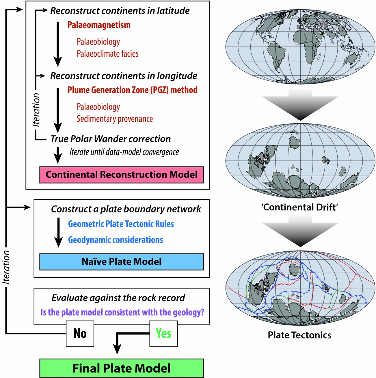
Figure 5. Simplified workflow for making pre-Jurassic plate models, as described in the text.
Of the tools available to make pre-Jurassic reconstructions, palaeomagnetism is by far the most important, and the only truly quantitative method. Palaeomagnetism is the study of the ancient magnetic field as it is preserved in rocks, and, owing to the dipolar nature of the time-averaged geomagnetic field (McElhinny, McFadden & Merrill, Reference McElhinny, McFadden and Merrill1996; Besse & Courtillot, Reference Besse and Courtillot2002; Evans, Reference Evans2006; Swanson-Hysell et al. Reference Swanson-Hysell, Maloof, Weiss and Evans2009), there is a unique relationship between magnetic inclination and latitude that can be used to convert a measured palaeomagnetic direction into palaeolatitude (Fig. 6a) (Tauxe, Reference Tauxe2010). As all magnetic directions should have originally pointed north (or south if the field was reversed), the palaeomagnetic declination can also be used to determine the azimuthal orientation that the continent was in at the time of magnetization acquisition. Because the geomagnetic field is axially symmetric, palaeolongitude is indeterminable from palaeomagnetic data, and palaeolongitude is thus the greatest uncertainty in pre-Jurassic plate models. However, the spatio-temporal distribution of palaeomagnetic data is also strongly heterogeneous, such that the palaeolatitude/orientation of a given continent may be likewise undefined for some (or all) of the modelled interval. Notably, in being inherently quantitative, palaeomagnetic data are complemented by a measure of uncertainty that is otherwise unique to pre-Jurassic reconstructive tools. Directional (spatial) errors occur at a variety of levels in palaeomagnetic analysis, but are often summarized at the study level as an ‘A95’, which is the angle from the computed mean within which 95% of the sample means lie (i.e. 2σ), assuming a Fisherian distribution (Fisher, Reference Fisher1953). Accompanying uncertainties in the age of the remnant magnetizations are typically more difficult to quantify (and are not likewise standardized), but a practical method of gauging and attenuating temporal errors from palaeomagnetic compilations is via the construction of apparent polar wander paths (APWPs), wherein palaeomagnetic data are merged and averaged by moving time-windows or spherical splines (Torsvik et al. Reference Torsvik, Van der Voo, Preeden, Mac Niocaill, Steinberger, Doubrovine, van Hinsbergen, Domeier, Gaina and Tohver2012).
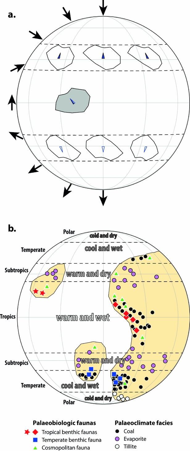
Figure 6. Methods for reconstructing ancient latitudes. (a) Palaeomagnetism. Observed magnetic inclinations from the grey continent can be used to restore it to a particular latitude (north or south, depending on the magnetic field polarity), shown by the dashed lines. The solid black arrows show the changing inclination angle from pole to pole in a normal-polarity, axial dipole field. The azimuthal orientation of the continent can be constrained by the magnetic declination (blue arrows), which originally pointed north or south (again, depending on the original field polarity). Longitude cannot be constrained by palaeomagnetism, so the various depicted positions of the reconstructed continent are all equally viable from the palaeomagnetic data alone. (b) Palaeoclimate facies and palaeobiology. Palaeoclimate facies (e.g. coals, evaporites, tillites, etc.) can allow a qualitative estimation of latitude as they tend to occur in particular climatic zones which are partly latitudinally controlled. Coals, for example, tend to form in the wet tropical and temperate belts, whereas evaporites are more common in subtropical arid belts. Palaeobiologic faunas can sometimes be used to infer latitude if they are temperature-sensitive. Palaeobiology may also be used to infer relative longitude (proximity) according to the similarity of benthic faunas. For example, similar temperate faunas are found on two formerly neighbouring blocks (blue squares), whereas dissimilar red tropical faunas (red stars and diamonds) indicate a significant separation of two landmasses, in this case by a large ocean. Note that cosmopolitan faunas are not generally useful for latitude or longitude determination.
Although palaeomagnetism is the only quantitative tool available for the determination of pre-Jurassic palaeolatitude, there are a number of other methods that can provide semi-quantitative or qualitative constraints on palaeolatitude and/or relative palaeolongitude (Fig. 6b). In some instances, fossils can provide both a qualitative estimate of the latitude of a continent – due to the latitude dependence of temperature – and its relative proximity to other blocks, according to the similarity of their faunas (Cocks & Fortey, Reference Cocks and Fortey1982; McKerrow & Cocks, Reference McKerrow and Cocks1986). However, the comparison of faunas needs to be made with some care and prudence, as common pitfalls – for example evaluating continent proximity by pelagic or cosmopolitan faunas – are rife in the literature. Palaeoclimatic indicators, notably evaporites, coals and tillites, can also be useful for estimating palaeolatitude, or for evaluating those established by palaeomagnetism (Irving & Briden, Reference Irving and Briden1962; Gordon, Reference Gordon1975; Scotese & Barrett, Reference Scotese, Barrett, McKerrow and Scotese1990; Evans, Reference Evans2006; Boucot et al. Reference Boucot, Xu, Scotese and Morley2013). Evaporites form most readily in subtropical arid belts on either side of the equator (presently between 20° and 30° N and S), whereas coals form along wet belts at the equator and mid-latitudes, and tillites are normally restricted to high latitudes (excepting periods of postulated global glaciation in the late Precambrian (Hoffman et al. Reference Hoffman, Kaufman, Halverson and Schrag1998)). Sedimentary provenance and correlative lithostratigraphy can also play a useful role in reconstructing conjugate continents, but again these tools must be used cautiously. For example, the discovery of highly similar detrital zircon records between two regions does not necessarily imply that they had a shared geologic history, or that the zircons themselves were derived from a common source (Andersen, Reference Andersen2014). Consequently, a consideration of possible transport pathways should be a prerequisite for drawing any source–sink connections (Thomas, Reference Thomas2011). Owing to the durability of zircon, sedimentary recycling can also play a dominant role in the shaping of provenance signatures, and may profoundly obscure true pre-existing spatio-temporal relationships (Andersen, Kristoffersen & Elburg, Reference Andersen, Kristoffersen and Elburg2016).
Our modern-day longitudinal reference system is an arbitrary human construct, and seafaring navigators struggled with a means to determine longitude long after the calculation of latitude was routine (Sobel, Reference Sobel2007). It should thus be unsurprising that the determination of longitude in the geologic past remains a great challenge. For the last ~120 Ma, palaeolongitude can be inferred from hotspot tracks, but prior to that time we lack direct palaeolongitude observables. Nevertheless, there have been several novel methodologies developed in the last decade which have opened new possibilities for palaeolongitude determination in deeper time. In the so-called subduction reference frame, if one assumes that subducted lithosphere sinks vertically, lithospheric slabs identified in the mantle by seismic tomography can be related back to a former subduction zone at the surface, and can thereby provide reconstructed subduction zones with palaeolongitudinal constraints (Van der Meer et al. Reference Van Der Meer, Spakman, Van Hinsbergen, Amaru and Torsvik2010) (Fig. 7a). However, although there have been proposals that this technique can be used back to possibly 300 Ma, objective global correlation exercises rather suggest that the temporal limit of this method lies between ~130 and 200 Ma (Domeier et al. Reference Domeier, Doubrovine, Torsvik, Spakman and Bull2016). An alternative approach that is applicable back to ~300 Ma is the ‘zero-longitude Africa’ reconstruction method of Burke & Torsvik (Reference Burke and Torsvik2004). This approach works by assuming that Africa – which probably moved the least in longitude of all plates since Pangaea break-up because it has been flanked by spreading ridges since that time – actually has not moved in longitude at all. If all the other plates are referenced to Africa in a global relative motion model, this allows the palaeolongitude of all the other plates to be determined. Although it is known that the palaeolongitude for Africa was not actually zero for the last 120 Ma (according to hotspot tracks (Doubrovine, Steinberger & Torsvik, Reference Doubrovine, Steinberger and Torsvik2016)), this approach acts to minimize the (unknown) global palaeolongitude error for earlier times.
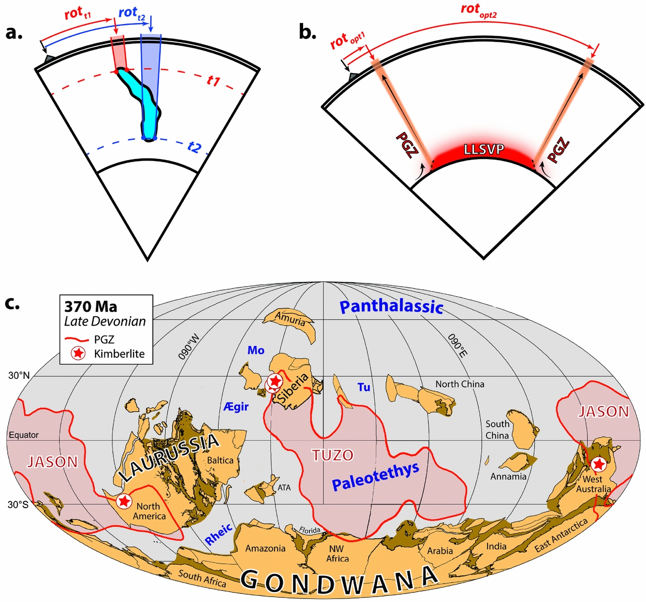
Figure 7. Methods for reconstructing ancient longitudes. (a) Subduction reference frame. A subducted lithospheric slab imaged by seismic tomography (irregular blue volume) is assumed to have sunk vertically from the surface following subduction, so that vertical projections of horizontal slices of that body (at depth) back to the surface reveal former locations of the subduction zone through time (red and blue fields). The age of the bottom of the slab, t 2 = onset of subduction, and the top of the slab, t 1 = cessation of subduction, may be dated directly from geological records, or by assuming an average slab sinking speed. Rotations can then be determined to restore the former active margin (grey triangle) to the appropriate locations at the appropriate times. (b) Plume generation zone (PGZ) reconstruction method. The large low shear velocity provinces (LLSVPs) at the base of the mantle (dubbed TUZO and JASON in (c); only one shown in (b)) are assumed to be stable, and plumes originate along their margins. Surface features related to plumes, namely large igneous provinces (LIPs) and kimberlites, can therefore be used to estimate the longitude of a continent at the time of their emplacement by assuming they erupted above one of the PGZs. The grey triangle represents a continent bearing a LIP or kimberlite; generally there will be some ambiguity in the restoration because there are multiple LLSVP margins (in the example shown, there are two equally plausible alternatives, opt1 and opt2). (c) Example reconstruction using the PGZ reconstruction method at 370 Ma. At this time kimberlites were intruded into West Australia and North America (linked to JASON), and Siberia (linked to TUZO). Although the reconstruction of any individual continent to an LLSVP margin would leave several options, by reconstructing them all together the alternative possibilities are greatly reduced.
The most promising methodology, and the only potential means of estimating absolute palaeolongitude prior to Pangaea formation, is the plume generation zone (PGZ) reconstruction method (Torsvik et al. Reference Torsvik, Van der Voo, Doubrovine, Burke, Steinberger, Ashwal, Trønnes, Webb and Bull2014). The PGZ method is based on the observation that most hotspots, large igneous provinces (LIPs) and kimberlites of the last 300 Ma, when reconstructed to their original palaeogeographic positions at the time of eruption, lie above the margins of the two large low shear velocity provinces (LLSVPs) below, in the lowermost mantle (Burke et al. Reference Burke, Steinberger, Torsvik and Smethurst2008; Torsvik et al. Reference Torsvik, Burke, Steinberger, Webb and Ashwal2010b). That observed correspondence suggests both that hotspots, LIPs and kimberlites are related to plumes sourced from the LLSVP margins and that the LLSVPs have remained effectively stable over the last 300 Ma. With that as a starting point, we pose the question: if the LLSVPs have been apparently stable since 300 Ma, why could they not have been stable for longer? Working from the assumption that the LLSVPs could have been stable prior to 300 Ma, one can exploit the observed relationship between LIPs, kimberlites and the LLSVP margins to use the occurrence of LIPs and/or kimberlites as a constraint on palaeolongitude in deeper time. In other words, continents bearing a LIP or kimberlite at a particular time need to be restored to a position such that they lay over one of the LLSVP margins at that time (Fig. 7b, c) (Torsvik et al. Reference Torsvik, Van der Voo, Doubrovine, Burke, Steinberger, Ashwal, Trønnes, Webb and Bull2014). If a LIP- or kimberlite-bearing continent is also constrained in latitude and orientation at the same time by palaeomagnetism (e.g. by palaeomagnetic data from a LIP or kimberlite), then the continent can be fully reconstructed. Notably, the selection of an LLSVP boundary in any isolated case would generally be arbitrary, but when working with the global assemblage of continents and following the ‘principle of least astonishment’ (i.e. Ockham's razor), often only one boundary is available or otherwise suitable. We stress again that LLSVP stability has only been demonstrated for the last 300 Ma, and our assumption of stability earlier in time has not been validated, but without this assumption it is impossible to estimate absolute palaeolongitude prior to 300 Ma. Obviously, further scrutiny and novel approaches to testing this assumption are of great importance.
A significant complication involved with use of the PGZ method is that reconstructions employing it must first be in a mantle reference frame. Because the entire solid Earth (crust and mantle) can rotate due to internal mass distribution changes – a process called true polar wander (TPW) (Gold, Reference Gold1955; Goldreich & Toomre, Reference Goldreich and Toomre1969) – the position and orientation of the LLSVPs can change with respect to the spin axis over time. Palaeomagnetic-based reconstructions, on the other hand, are referenced directly to the spin axis. This means that time-dependent TPW needs to be removed from palaeomagnetic reconstructions (or, equivalently, added to the mantle reference frame) in order to allow direct comparison between a palaeomagnetic-based continental reconstruction and the deep mantle LLSVPs – and thus to employ the PGZ method. As a net rotation of the entire solid Earth, TPW can be identified from the residual of globally integrated plate motions for any given time (i.e. the net displacement field from the summed plate motions) (Jurdy & Van der Voo, Reference Jurdy and Van der Voo1975), but this approach introduces several problems. Firstly, because such a calculation requires first knowing global plate motions, the determination of TPW and the determination of palaeolongitude by the PGZ method present heavily convolved problems that can only be solved iteratively (Torsvik et al. Reference Torsvik, Van der Voo, Doubrovine, Burke, Steinberger, Ashwal, Trønnes, Webb and Bull2014). TPW is recalculated from the global plate velocity field according to new longitudinal adjustments, which results in a new TPW correction, in turn necessitating new longitudinal adjustments. The aim is to reach a time-dependent TPW estimate that appropriately restores the plates to the longitudes required by the PGZ method for each time. A second problem is that, for pre-Jurassic time, the oceanic lithosphere is missing, so TPW estimates can only be based on the global continental velocity field (Steinberger & Torsvik, Reference Steinberger and Torsvik2008) (and so too the iterative approach just described). Finally, it is also possible that a net rotation observed from globally integrated plate motions is due to a net rotation of the lithosphere (NR) (Conrad & Behn, Reference Conrad and Behn2010; Torsvik et al. Reference Torsvik, Steinberger, Gurnis and Gaina2010a), which differs from TPW in that the underlying mantle does not participate. The latter two problems can be overcome by exploiting the observation that, at least for the last ~300 Ma (during part of which we can distinguish between NR and TPW with reference to hotspot tracks), the predominant axis of TPW (0°, ~11°E) was closely associated with the major axis of Earth's geoid, which passes nearly through the centroids of the LLSVPs (Torsvik et al. Reference Torsvik, Van der Voo, Preeden, Mac Niocaill, Steinberger, Doubrovine, van Hinsbergen, Domeier, Gaina and Tohver2012). If the LLSVPs were stable in earlier times, it is likely that the axis of TPW was too. By fixing the axis of TPW, the estimation of its time-dependent magnitude from the continental velocity field becomes more robust, and it may be possible to discriminate between TPW and NR (where the latter is not about an axis similar to that assumed for TPW).
4. Playing by ‘the rules’
With the time-dependent palaeogeography of the continents established, work can proceed on the reconstruction of plate boundaries, and finally the construction of full tectonic plates. The reconstruction of plate boundaries can be achieved both through the application of plate tectonic ‘rules’, and from the analysis of continental margin geology. In general, both of these approaches are essential. In practice, plate boundary reconstruction is often a highly iterative process, and while it is not necessary to start with the application of plate tectonic rules (as opposed to starting from the continental margin geology), for the purposes of this discussion it will be informative to do so. What therefore follows is an explanation of how we can use plate tectonic rules, applied to our now-completed continental rotation model, to estimate the nature, location and orientation of plate boundaries. Importantly, this is done without reference to the rock record, and so these plate boundaries can be considered ‘naïve’ (uninformed). While it may initially seem futile to generate such naïve boundaries, this exercise presents an important illustration of the wealth of additional information – implicit to any given continental rotation model – that is almost always discarded; the value of this information thus appears widely under-appreciated. In the next section, we improve our naïve plate boundary network by testing it against the continental rock record (Fig. 5).
The oft-cited ‘rules’ of plate tectonics can be divided into two types: geometric and dynamic. The geometric rules are few and simple, but powerful. The most fundamental of these is area conservation. Because both the volume and shape of the Earth have remained effectively constant since at least the Archaean, the surface area of the planet must also have remained constant over that time. The global surface area consumed by subduction per unit time in a plate model must therefore be balanced by the global surface area generated by ridges in the model. Because most reconstruction software operates by default on a fixed-area spherical surface, this conservation law is commonly pre-assured and so may seem inconsequential. However, this conservation law holds at any arbitrary scale (so long as deformation is negligible), and it is at smaller scales that this rule becomes very useful. Where two continents are moving apart, for example, a spreading centre is required to develop (here, and in the following, we assume continents and plates are purely rigid), and this will be true whether or not we have direct observational evidence of that former boundary (Fig. 8). Likewise, in the zone between two converging blocks, subduction must occur.
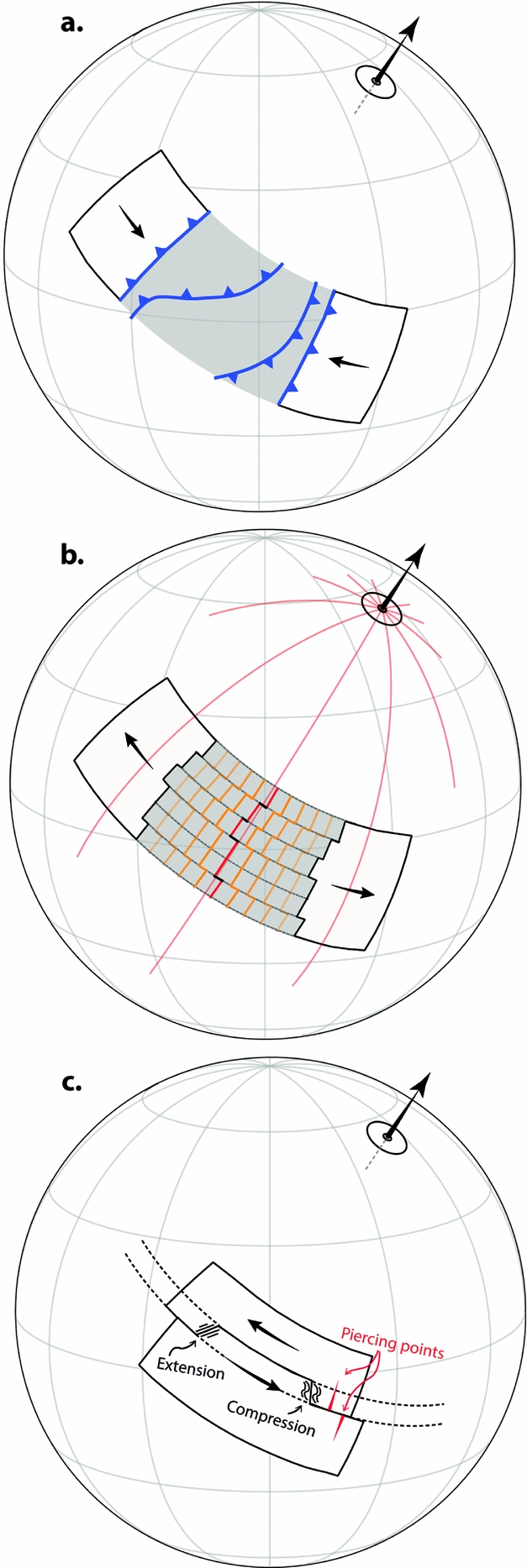
Figure 8. Basic plate tectonic rules concerning plate boundaries. In each of the three examples ((a) convergent, (b) divergent and (c) transform), relative motion between the plates is described by the depicted Euler pole. (a) Convergent boundaries are not geometrically required to follow any orientation with respect to the Euler pole (four equally valid alternatives among the innumerable possibilities are shown), but must fully traverse the converging area (grey region). (b) Divergent boundaries tend to align themselves along the trace of a great circle passing through the Euler pole (red lines); transform segments offsetting the ridge will follow small circles about the Euler pole (dotted black lines). Spreading along the ridge is assumed to be symmetrical, so the location of the ridge is predictable if the motions of the flanking continents are known. (c) Transform boundaries follow small circles about the Euler pole (dashed lines); deviations from the small circle traces result in extension or compression. Where both margins are preserved, piercing points can be used to establish the sense and magnitude of motion along the boundary.
Though area conservation may require a spreading ridge or subduction zone to occur in a region between two continents, it does not specify where that boundary must be for any time other than when the blocks are infinitesimally close (at which point the ridge or trench must occur along their shared boundary). In the scenario of two converging blocks prior to collision, the trench could lie along the inner edge of either of the blocks, or it could occur as an intraoceanic subduction system anywhere in between them (Fig. 8a). Indeed, geometry stipulates only that the convergent boundary must fully transect the converging area (normal to the convergence direction), but this can be via any path. Thus, all such possibilities are equally plausible geometrically, but there will of course be strong distinctions in which scenarios are most dynamically plausible. And, most importantly, there may be direct geologic evidence that can be used to evaluate these alternatives, as discussed in the next section.
Ridges, like subduction zones, are not geometrically required to assume any particular orientation between a pair of diverging plates, but they commonly tend to align themselves approximately perpendicular to the direction of spreading – or, expressed another way, they tend to follow the trace of a great circle which lies in the same plane as the rotation axis that defines the relative motion of the bounding plates (Fig. 8b). There is also no geometric reason why spreading along a ridge should necessarily be symmetrical, but from global observations of extant oceanic crust it appears that approximately symmetrical spreading is a reasonable first-order assumption for spreading ridges in major ocean basins (except back-arc basins) (Müller et al. Reference Müller, Sdrolias, Gaina and Roest2008). In particular, there appears to be no general correlation between absolute plate motion velocities and spreading asymmetry, and strong spreading asymmetries outside of back-arc basins are largely attributable to the local influence of hotspots (Müller et al. Reference Müller, Sdrolias, Gaina and Roest2008). Given these two simple assumptions – that ridges tend to align themselves perpendicular to the direction of spreading and that spreading is symmetrical – it is straightforward to determine the position and orientation of a ridge between a pair of diverging blocks and to track it through time, so long as the motions of the diverging blocks themselves are known.
Unlike ridges and trenches, the orientation of transform boundaries is geometrically constrained as long as they are defined as boundaries of pure slip. Such boundaries are always parallel to the relative motion vector of their bounding plates, meaning that they are confined to the trace of a small circle about the Euler pole describing the relative plate motion (Fig. 8c). Deviations from that path are necessarily deviations from the condition of pure slip, and will result in compression or extension, depending on the sense of relative motion. This is a particularly powerful observation because it means that transform boundaries, where they can be recognized in the rock record, can be used to locate Euler poles directly.
Dynamic considerations are inherently looser than the geometric rules of plate tectonics, but are nonetheless critical to the task of constructing pre-Jurassic plate tectonic models. Arguably, the most useful of these is the concept of a plate tectonic ‘speed limit’ (Meert et al. Reference Meert, Van der Voo, Powell, Li, McElhinny, Chen and Symons1993; Zahirovic et al. Reference Zahirovic, Müller, Seton and Flament2015). By establishing the maximum theoretical velocity of plates, one can immediately reject countless alternative models which, while otherwise conforming to geometric and geologic constraints, would require plates to move at rates in excess of that threshold. Unfortunately, the true plate tectonic speed limit is unknown. The global mean plate speed over the last 200 Ma was ~4 cm a−1 (Zahirovic et al. Reference Zahirovic, Müller, Seton and Flament2015), but that figure masks significant variability, including the notoriously fast Cretaceous–Palaeogene motion of India, which reached velocities in excess of 18 cm a−1 (Klootwijk et al. Reference Klootwijk, Gee, Peirce, Smith and McFadden1992). That variability has been ascribed to differences in the make-up of plates and the types of boundaries that circumscribe them, with the fastest plates being mostly oceanic and actively subducting, and the slowest plates having a greater continental area and lacking active margins (Schult & Gordon, Reference Schult and Gordon1984; Zahirovic et al. Reference Zahirovic, Müller, Seton and Flament2015). But whether those trends are time-independent and thus broadly applicable to times prior to ~200 Ma remains unclear (Meert et al. Reference Meert, Van der Voo, Powell, Li, McElhinny, Chen and Symons1993; Gurnis & Torsvik, Reference Gurnis and Torsvik1994). Still, as a practical tool, plate speed minimization presents an important semi-quantitative means of independent model evaluation, and very high plate speeds (>30 cm a−1) should be considered suspicious.
Drawing on knowledge gleaned from numerical and analytical models as well as studies of Mesozoic–Cenozoic plate motions (Forsyth & Uyeda, Reference Forsyth and Uyeda1975; Cloos, Reference Cloos1993; Lithgow-Bertelloni & Richards, Reference Lithgow-Bertelloni and Richards1998; Conrad & Lithgow-Bertelloni, Reference Conrad and Lithgow-Bertelloni2002), Stampfli & Borel (Reference Stampfli and Borel2002) introduced the concept of using presumed plate driving forces (specifically slab-pull and slab buoyancy) to inform plate reconstructions. Such an approach thus entails the formulation and evaluation of alternative geodynamic scenarios (whether conceptual or quantitative) as part of the plate boundary construction process. This approach is very useful, particularly in regions of time and space where physical constraints may otherwise be altogether lacking, but it is essential to proceed prudently, and with the recognition that our understanding of the plate driving forces is both incomplete and temporally biased. Notably, Stampfli & Borel (Reference Stampfli and Borel2002) (and many derivative works) ignore the contribution of mantle dynamics to the motion of plates, despite the fact that plumes appear to have played a prominent (if not central) role in continental break-up (Buiter & Torsvik, Reference Buiter and Torsvik2014), the reorganization of oceanic plates (Chandler et al. Reference Chandler, Wessel, Taylor, Seton, Kim and Hyeong2012) and the redirection of plate motions in several examples in the last 300 Ma (Torsvik & Cocks, Reference Torsvik and Cocks2017).
Another useful consideration concerns the trench-perpendicular motion of subduction zones, which (if not stationary) can be classified as ‘retreating’ (away from the overriding plate) or ‘advancing’ (towards the overriding plate). Both retreating and advancing trenches are observed on Earth, in analogue experiments and in numerical simulations (Jarrard, Reference Jarrard1986; Royden & Husson, Reference Royden and Husson2006; Schellart et al. Reference Schellart, Freeman, Stegman, Moresi and May2007; Di Giuseppe et al. Reference Di Giuseppe, Van Hunen, Funiciello, Faccenna and Giardini2008; Funiciello et al. Reference Funiciello, Faccenna, Heuret, Lallemand, Di Giuseppe and Becker2008; Stegman et al. Reference Stegman, Farrington, Capitanio and Schellart2010), but in general retreating trenches appear to be preferred, as could be expected from a simple subduction system driven by negative slab buoyancy (Schellart, Stegman & Freeman, Reference Schellart, Stegman and Freeman2008). From contemporary plate motions, Schellart, Stegman & Freeman (Reference Schellart, Stegman and Freeman2008) found ~62–78% of trenches to be retreating, and Williams et al. (Reference Williams, Flament, Müller and Butterworth2015) showed that over the last 130 Ma, the ratio of trench retreat to advance was ~2:1, but with notable temporal variation. However, as also pointed out by Schellart, Stegman & Freeman (Reference Schellart, Stegman and Freeman2008), strong trench migration (either retreating or advancing) is not generally expected as it necessitates displacement of large volumes of upper mantle material, and so a minimization of trench-perpendicular motion should be preferred.
Other applicable dynamic considerations relate to theoretical expectations for NR and TPW, which we present as a means of model evaluation in Section 6.
5. Looking to the rocks
At this point we have properly reconstructed the continents and generated a plate boundary network around them, such that we have a fully functional, albeit naïve, plate model. This plate model is now to be tested against the continental rock record, and where the model is in conflict with the geological observations, modifications must be made (Fig. 5). Importantly, all revisions to the plate boundary network require reconsideration of the tasks performed earlier. That is to say, any modifications to the plate boundary network must be made in compliance with the aforementioned plate tectonic rules, in the specific context of the underlying continental rotation model. In some instances the continental geology and plate tectonic constraints together indicate that a revision to the underlying continental rotation model is necessary (in supplying novel palaeogeographic information, such instances are a clear demonstration of why full-plate models are superior to their continental drift precursors). Testing of the naïve plate model and the progressive construction of an ‘informed’ plate model by incorporation of geologic data is thus an iterative process.
The geologic data which are most valuable for such testing are those which communicate information about relative plate motion and marginal plate dynamics. Often the clearest records are those from former active margins, which can be marked by arc-related igneous rocks, HP-UHP metamorphic rocks, accretionary complexes, ophiolites and nappes. Where the original structural relationships of those features can be unambiguously established – the magmatic arc, accretionary complex and HP-UHP metamorphic belt, for example – the polarity of subduction can be determined (Dickinson, Reference Dickinson1971; Stern, Reference Stern2002). The age of onset and cessation of subduction can also be constrained by those records; for example, the first appearance of arc-related magmatism or of a supra-subduction ophiolite provides a minimum onset age, whereas syn-orogenic intrusions, the appearance of molasse, the transport of nappes or the beginning of HP-UHP metamorphism can reflect a collision.
Geologic records of divergent margins from pre-Jurassic time are inherently more limited because unlike trenches, which are approximately fixed to the overriding plate, spreading centres are mobile with respect to both plates. Direct records of divergent margins from continental margin geology are therefore restricted to relics of pre-drift rifting and break-up-related magmatism, and are succeeded by the development of a passive margin (Lister, Etheridge & Symonds, Reference Lister, Etheridge and Symonds1986; Bradley, Reference Bradley2008; Peron-Pinvidic, Manatschal & Osmundsen, Reference Peron-Pinvidic, Manatschal and Osmundsen2013). Those relics provide excellent constraints on the nascent development of a divergent margin, but the ability to directly track its evolution from the continental margin geology is quickly lost with the onset of seafloor spreading. Nevertheless, the persistence and maturation of passive margins themselves can provide useful information, not the least of which is a clear demarcation of where tectonic boundaries cannot lie. Passive margins can also be useful in locating former rift zones where syn-rift sequences may not be obvious, as nearly all passive margins were pre-dated by marginal rifting (the exceptions being ‘sheared passive continental margins’ (Scrutton, Reference Scrutton and Scrutton1982)) (Bradley, Reference Bradley2008).
Transform boundaries are typically the most difficult to recognize from the rock record, and particularly so for pre-Jurassic time because the once-conjugate margins that define such boundaries are generally no longer in contact. Where a fossil transform is preserved between two blocks that have remained in contact along their shared (and now extinct or dormant) boundary, the former relative motion can often be worked out from the identification of piercing points, or features that have been offset along that boundary (Fig. 8c). This is critical because although the trend of a transform boundary constrains the orientation of the Euler pole (as described above), it does not constrain the sense of motion, which can be either dextral or sinistral. However, even in the general case where only one margin of a former transform boundary remains, the sense of motion along that boundary can often be surmised because transforms on Earth are never ‘perfect’. They often deviate from the trace of a pure-slip boundary, resulting in restraining and releasing bends, and thus zones of transpression and transtension, respectively (Teyssier, Tikoff & Markley, Reference Teyssier, Tikoff and Markley1995; Dewey, Holdsworth & Strachan, Reference Dewey, Holdsworth, Strachan, Holdsworth, Strachan and Dewey1998). Where such zones can be recognized together with respect to the main transform boundary, they can be used to infer the former sense of motion. Such analysis is best performed at the margin scale, but where records are only regionally or locally preserved, even outcrop-scale kinematic indicators can be used to evaluate or inform a plate model (Simpson & De Paor, Reference Simpson and De Paor1993).
6. State of the art and future directions
The first pre-Jurassic full-plate model was produced at the University of Lausanne, Switzerland, under the direction of Gérard Stampfli, whose group first introduced the concept of making reconstructions with ‘dynamic plate boundaries’ (Stampfli & Borel, Reference Stampfli and Borel2002). A recent version of their model (Hochard, Reference Hochard2008; Vérard et al. Reference Vérard, Hochard, Baumgartner, Stampfli and Liu2015; hereafter ‘UL’ model) extends back to 600 Ma (with true global coverage extending back to ~460 Ma) and includes synthetic isochrons, but was constructed under a Baltica-fixed (back to 400 Ma) or Gondwana-fixed (from 400 to 600 Ma) reference frame, without absolute longitude constraints. Most problematic, however, is that the UL model was sold to industry in 2010, and so the details are proprietary and thus inaccessible to the wider scientific community. Following that pioneering work, Domeier & Torsvik (Reference Domeier and Torsvik2014) published the first publicly released pre-Jurassic plate model, which specifically spanned the late Palaeozoic, extending from 410 to 250 Ma. That model, which is based on the continental rotation model and PGZ reconstruction method presented by Torsvik et al. (Reference Torsvik, Van der Voo, Doubrovine, Burke, Steinberger, Ashwal, Trønnes, Webb and Bull2014), also represents the first pre-Jurassic plate model with absolute longitudes. Subsequently, Domeier (Reference Domeier2016) presented an early Palaeozoic (500–410 Ma) regional plate model with absolute longitudes for the Iapetus and Rheic domains (flanked by Laurentia, Baltica and west Gondwana), as part of an ongoing initiative to build a global early Palaeozoic plate model. With the aim of bridging the late Palaeozoic model of Domeier & Torsvik (Reference Domeier and Torsvik2014) with Jurassic to modern (200–0 Ma) plate models, Matthews et al. (Reference Matthews, Maloney, Zahirovic, Williams, Seton and Müller2016) presented a new Triassic plate model and modified Domeier & Torsvik (Reference Domeier and Torsvik2014) and Seton et al. (Reference Seton, Müller, Zahirovic, Gaina, Torsvik, Shephard, Talsma, Gurnis, Turner and Maus2012) to produce a merged plate model that extends from 410 Ma to the present day. Most recently, Merdith et al. (Reference Merdith, Collins, Williams, Pisarevsky, Foden, Archibald, Blades, Alessio, Armistead and Plavsa2017) presented a plate model for the Neoproterozoic (1000–520 Ma), although without absolute longitude constraints. Much ground-laying work therefore remains to be done, in particular on the completion of an early Palaeozoic global model and the determination of absolute palaeolongitude in the Neoproterozoic.
In addition to the construction of new models, much also remains to be done on the testing and refinement of existing models. One particularly powerful aspect of full-plate models is their capacity to make novel and quantitative palaeomagnetic predictions, which can be directly validated (or rejected) by the acquisition of new data. But how can these plate models, which are underpinned by palaeomagnetic data, generate truly novel palaeomagnetic predictions (i.e. predictions that are not already directly borne out by existing palaeomagnetic data)? The reason is that these models have been infused with additional information derived from plate tectonic principles and from the geologic record. As an example, no reliable palaeomagnetic data are published for any of the pre-Jurassic blocks of Afghanistan, and so their palaeolatitudes are entirely unconstrained by that method. Nevertheless, the geologic records of those blocks reveal that they were part of an elongate ribbon continent (Cimmeria) that broke away from the northern margin of Gondwana in the Permian in response to subduction of the Palaeotethys Ocean to the north (Fig. 9a, b) (Şengör, Reference Şengör1984; Stampfli, Reference Stampfli, Bozkurt, Winchester and Piper2000). Because other terranes of Cimmeria have yielded late Palaeozoic – early Mesozoic palaeomagnetic data, namely the Iranian and Tibetan terranes (Huang et al. Reference Huang, Opdyke, Peng and Li1992; Muttoni et al. Reference Muttoni, Mattei, Balini, Zanchi, Gaetani, Berra, Brunet, Wilmsen and Granath2009), the palaeogeography of the Afghan blocks can be established indirectly. And although indirect, that restoration is quantified in the plate model, such that synthetic (predicted) palaeomagnetic directions can be generated for any location among those blocks, for any modelled time (Fig. 9c). By testing such novel predictions against new data, the veracity of a plate model can be critically evaluated in a way never before possible.
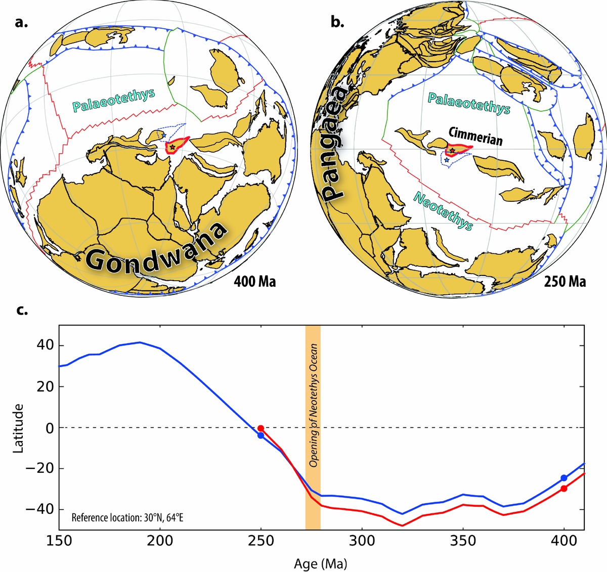
Figure 9. Example of predictive power of full-plate models. (a, b) Full plate reconstructions at 400 and 250 Ma (Domeier & Torsvik, Reference Domeier and Torsvik2014) showing the location and tectonic context of the central Afghan terranes, outlined in red; blue dashed outline is the position of the same terrane in Matthews et al. (Reference Matthews, Maloney, Zahirovic, Williams, Seton and Müller2016). (c) Predicted palaeolatitude of a reference location (starred) in the central Afghan terrane, derived from Domeier & Torsvik (Reference Domeier and Torsvik2014) (410–250 Ma, red curve) and Matthews et al. (Reference Matthews, Maloney, Zahirovic, Williams, Seton and Müller2016) (410–150 Ma, blue curve). The yellow band at ~275 Ma marks the opening of the Neotethys Ocean, which resulted in the rifting of the Cimmerian ribbon continent (including the central Afghan terranes) from northern Gondwana.
Another possible means to test this new generation of plate models involves taking advantage of the full kinematic definition of ridges and plates to generate synthetic isochrons and oceanic age grids (Müller et al. Reference Müller, Sdrolias, Gaina and Roest2008). With an oceanic age grid it is straightforward to track the age of the oceanic lithosphere as it subducts anywhere at any time, presenting a powerful opportunity to check the model against available ophiolite generation and emplacement ages. This potential is particularly attractive in that it could offer direct constraints on the location of ridges that may otherwise be inscrutable. It is worth noting, however, that many (if not most) ophiolites appear to be of supra-subduction origin (Pearce, Lippard & Roberts, Reference Pearce, Lippard, Roberts, Kokelaar and Howells1984; Metcalf & Shervais, Reference Metcalf, Shervais, Wright and Shervais2008; Whattam & Stern, Reference Whattam and Stern2011), and are thus of limited use in constraining the position of ancient ridges.
A third and rather more precarious approach to testing and refining global plate models involves optimization of the time-dependent global plate velocity field according to some expectations related to TPW and/or NR. TPW is associated with a time-dependent, often non-zero angular displacement. Theoretically, the spin axis may move (with respect to the solid Earth) as much as 1–2° Ma−1 (Tsai & Stevenson, Reference Tsai and Stevenson2007; Steinberger & Torsvik, Reference Steinberger and Torsvik2010), but the Phanerozoic pattern of TPW, as determined from the continental rotation model of Torsvik et al. (Reference Torsvik, Van der Voo, Doubrovine, Burke, Steinberger, Ashwal, Trønnes, Webb and Bull2014), is dominated by slow (<1° Ma−1) oscillatory swings around approximately the same axis (0°N, ~11°E). The maximum net TPW angle (deviation from the present location of the spin axis) for the past 410 Ma is estimated to be 31° (Fig 10a). However, it is not straightforward to determine Palaeozoic TPW before the Carboniferous (~350 Ma) because the continental masses are dominantly at polar latitudes in the southern hemisphere (e.g. Fig. 9a). It is therefore more difficult to differentiate between plate motion and TPW without assuming a specific location for Earth's minimum inertial axis, which we assume to be at 0°N, ~11°E, as in late Palaeozoic–Mesozoic time.
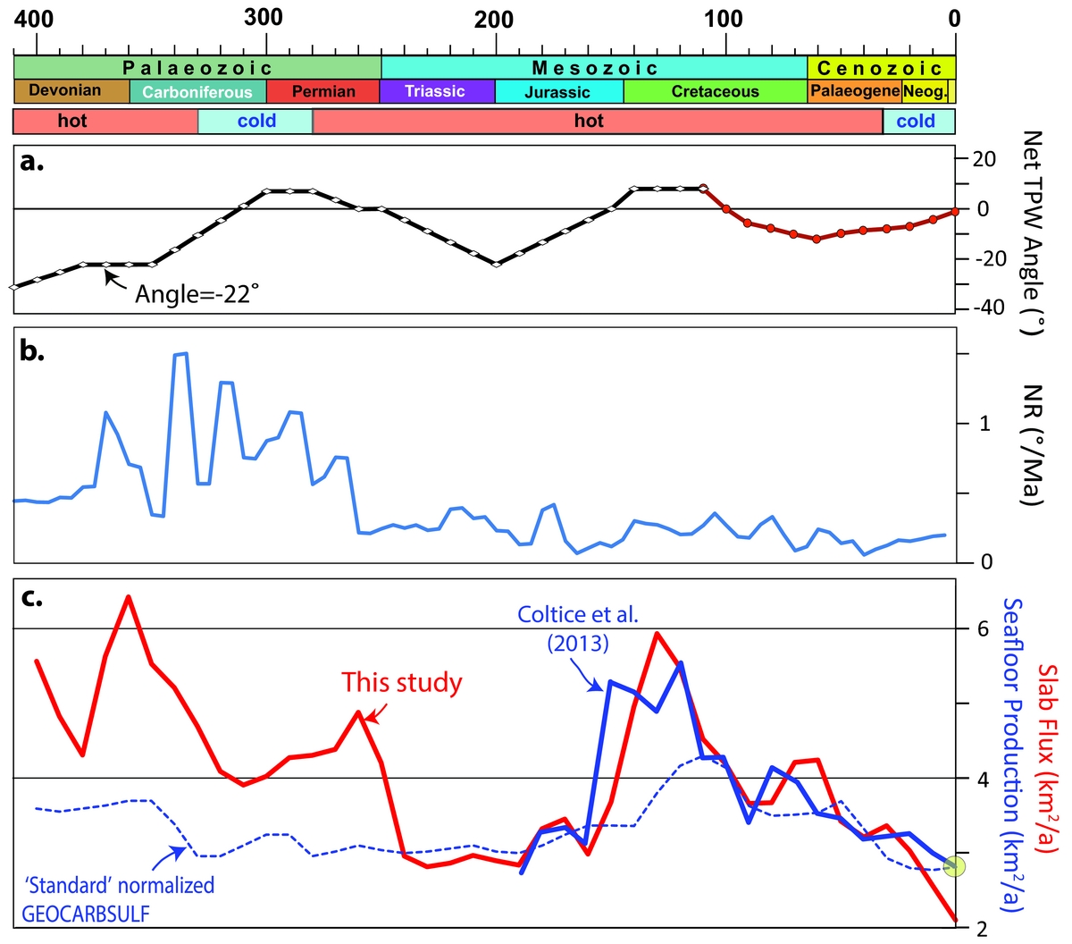
Figure 10. Phanerozoic timescale, icehouse (cold) versus greenhouse (hot) conditions (Torsvik & Cocks, Reference Torsvik and Cocks2017), and estimates of true polar wander (TPW), net lithosphere rotation (NR) and subduction flux since 410 Ma. (a) Net TPW angle (deviation from the present location of the spin axis) estimated from palaeomagnetic data (410–110 Ma; Torsvik et al., Reference Torsvik, Van der Voo, Doubrovine, Burke, Steinberger, Ashwal, Trønnes, Webb and Bull2014) and from a direct comparison of palaeomagnetic and hotspot reference frames (Doubrovine, Steinberger & Torsvik, Reference Doubrovine, Steinberger and Torsvik2012) for the last 110 Ma. (b) Net lithosphere rotation (based on Domeier & Torsvik, Reference Domeier and Torsvik2014; Matthews et al. Reference Matthews, Maloney, Zahirovic, Williams, Seton and Müller2016). (c) Subduction flux calculated from a full-plate model for the past 410 Ma (red line: Domeier & Torsvik, Reference Domeier and Torsvik2014; Matthews et al. Reference Matthews, Maloney, Zahirovic, Williams, Seton and Müller2016). Subduction flux estimates are compared with a seafloor production curve for the past 200 Ma (blue line: Coltice et al. Reference Coltice, Seton, Rolf, Müller and Tackley2013). The stippled blue line is the GEOCARBSULF standard curve for normalized seafloor production (ƒSR parameter) and here normalized to the Coltice et al. (Reference Coltice, Seton, Rolf, Müller and Tackley2013) estimate of present-day seafloor production.
In the course of the construction of a new continental rotation model, TPW must be re-estimated (as the final estimate in the iterative approach to solving the convolved problems of TPW correction and PGZ longitude restoration; Fig. 5), but this estimate is only determined from the continental velocity field in times prior to the mid-Cretaceous. If the subsequent construction of plate boundaries (and thus the oceanic portions of plates) is done without consideration of this TPW estimate, the resulting global plate velocity field will almost certainly differ from it. By default, the boundaries defining large oceanic plates for which there is little or no direct evidence should be designed in the simplest manner possible. An alternative approach could thus endeavour to design the entirely synthetic plates in such a way that the globally integrated plate motions yield a residual (that is, TPW) which is the same as or highly similar to that determined from the continental motions alone.
Estimating NR is important in geodynamic modelling, and the basic assumption is that NR should be zero unless individual lithospheric plates have different couplings to the underlying asthenosphere (O'Connell, Gable & Hager, Reference O'Connell, Gable, Hager, Sabadini, Lambeck and Boschi1991; Ricard, Doglioni & Sabadini, Reference Ricard, Doglioni and Sabadini1991). But most plate models for recent times predict varying degrees of westward drift of the lithosphere with respect to the deep mantle (Gordon & Jurdy, Reference Gordon and Jurdy1986; Conrad & Behn, Reference Conrad and Behn2010; Torsvik et al. Reference Torsvik, Steinberger, Gurnis and Gaina2010a). NR since 30 Ma has varied between 0.1° and 0.2° Ma−1 and fluctuations in NR before that time – with peaks approaching 0.5° Ma−1 in the Mesozoic and exceeding 1° Ma−1 in the Palaeozoic (Fig. 10b) – are probably artificial variations caused by the design of the synthetic oceanic plates (Torsvik & Cocks, Reference Torsvik and Cocks2017). Because NR can be defined as any remaining residual from the globally integrated plate motions after TPW correction, the oceanic plates could also be designed to minimize this residual.
The significant shortcoming of these approaches, however, is that the continents alone may not accurately portray TPW and/or NR, and so endeavouring to construct oceanic plate polygons to match a TPW/NR estimate derived from global continental motions could be deleterious. Similarly, if the axis of TPW is not approximately fixed over time as we have assumed here, TPW estimates will be erroneous and so too any plate models constructed to comply with them. TPW is driven by changes to Earth's internal mass distribution, and is notably sensitive to subduction at intermediate to high latitude (Steinberger & Torsvik, Reference Steinberger and Torsvik2010), so an alternative and more rigorous approach to constructing a plate model consistent with continental TPW estimates would be to ensure that the global framework of subduction in the model could drive the integrated motion observed from the continents. However, this would entail iterative refinements to a plate model paired with numerical simulations, which would be laborious, and a systematic study of how subduction zone locations relate to TPW (Steinberger & Torsvik, Reference Steinberger and Torsvik2010) has never been attempted for pre-Mesozoic times.
The testing of pre-Jurassic plate models by the predictions that they yield is particularly important in that it is not generally straightforward to assign quantitative error estimates to these models, or rather to their constituent Euler poles. For plate models of the last ~200 Ma, statistical tools have been developed to quantify and propagate the rotational uncertainties associated with the relative fitting of marine magnetic anomalies and fracture zones (Hellinger, Reference Hellinger1981; Molnar & Stock, Reference Molnar and Stock1985; Chang, Reference Chang1988; Kirkwood et al. Reference Kirkwood, Royer, Chang and Gordon1999), and they have also been applied to estimate the rotational uncertainties in the fitting of hotspot tracks (O'Neill, Müller & Steinberger, Reference O'Neill, Müller and Steinberger2005; Doubrovine, Steinberger & Torsvik, Reference Doubrovine, Steinberger and Torsvik2012). But as pre-Jurassic oceanic crust and hotspot tracks have been lost to subduction, these statistical tools are not readily useful in reconstructions of the pre-Jurassic world. As noted above, concerning pre-Jurassic reconstructive methods, explicit quantitative uncertainties are only routinely provided by paleomagnetic data, which constrain only continental latitude and azimuthal orientation. Because the estimation of palaeolongitude is accomplished by qualitative to semi-quantitative means generally lacking defined uncertainty estimates, the routine assignment of error to pre-Jurassic Euler poles is problematic. Conceivably, if uncertainty estimates could be assigned to each palaeolongitude determination, error estimates could be derived for the Euler poles and propagated where necessary. However, it is not clear how this could be feasibly achieved at present. Estimates of the uncertainty of palaeolongitude reconstructions based on faunas and facies, for example, would be very difficult to formulate objectively. Conversely, application of a uniform uncertainty for all palaeolongitude estimations based on such data would mask the immense variability in the quality of those determinations. Palaeolongitude estimates by the PGZ reconstruction method are perhaps the most amenable to a standardized uncertainty quantification, but as the hypothesis of long-term LLSVP stability itself remains to be validated, a consideration of such error estimation seems premature. Given these impediments to meaningful error estimation, we contend that the most practical way to evaluate pre-Jurassic plate models is by testing the predictions that they present. The problem of rigorous error estimation clearly poses an outstanding challenge for the future.
Although the capacity of full-plate models to provide testable predictions is critical, ultimately their function should extend further, to provide novel information about events or processes that may otherwise be inscrutable. It is not our intention here to try to explore this very large and still uncharted opportunity space, most of which will require further modelling with the employment of full-plate models as an input. Nevertheless, some tantalizing questions that may now be approachable include: Is there a persistent pattern in global plate motions across Wilson Cycles (Conrad, Steinberger & Torsvik, Reference Conrad, Steinberger and Torsvik2013)? Does the broad planform of mantle convection evolve on the timescale of mantle overturn (~150–200 Ma) (Zhong et al. Reference Zhong, Zhang, Li and Roberts2007)? Can we observe telling trends in possible climate-forcing mechanisms over hundreds of millions of years (Van der Meer et al. Reference Van Der Meer, Zeebe, van Hinsbergen, Sluijs, Spakman and Torsvik2014)? As a brief example of the latter (or, flagrant speculation in lieu of detailed modelling), we note that seafloor spreading can be used to gauge tectonic contributions to the global atmospheric CO2 budget (Sano & Williams, Reference Sano and Williams1996; Marty & Tolstikhin, Reference Marty and Tolstikhin1998; Van der Meer et al. Reference Van Der Meer, Zeebe, van Hinsbergen, Sluijs, Spakman and Torsvik2014), and so the time-dependent seafloor production rate (SPR) is a key parameter in the estimation of past CO2 fluxes. For the past 84 Ma (since the end of the Cretaceous Normal Superchron), the SPR can be calculated directly and with confidence from marine magnetic anomalies (e.g. Coltice et al. Reference Coltice, Seton, Rolf, Müller and Tackley2013), whereas prior to that we must turn to indirect means. One possible indication of a change in SPR is a change in sea level, and the ‘standard’ estimate of SPR in the GEOCARBSULF climate model is estimated from sea-level inversions before the Jurassic (Berner, Reference Berner2004; Royer, Reference Royer2014). Alternatively, with a global plate model, the time-dependent SPR (or, equivalently on our fixed-area planet, the subduction flux) can be extracted directly. In Figure 10c we compare the SPR of the standard curve with our new estimate derived from the plate model of Matthews et al. (Reference Matthews, Maloney, Zahirovic, Williams, Seton and Müller2016). Our estimate is at times much higher than the standard curve, but using our estimates in place of the standard curve in GEOCARBSULF (without changing any other parameters) results in CO2 levels of 500–550 ppm in the Late Carboniferous – Early Permian, which is close to the estimated threshold (Lowry et al. Reference Lowry, Poulsen, Horton, Torsvik and Pollard2014) to allow continental-scale glaciations at that time.
To close, we express the hope that the arguments made and methodology described here will encourage others to endeavour to make, test and/or revise palaeogeographic models based on plate tectonics rather than continental drift. The construction of such models, particularly on a global scale, is a colossal task – and so to get the grand puzzle of our dynamic Earth properly reassembled in both space and time will require input from across our broad community.
Acknowledgements
We thank Peter Cawood and an anonymous reviewer for comments that improved the manuscript. This work was supported by the Research Council of Norway (RCN), through its Centres of Excellence funding scheme, project number 223272 (CEED), and through RCN project 250111 to M.D.


