


1. Introduction
The Sonoma Foreland Basin (SFB, western USA; Fig. 1a) provides an excellent Early Triassic fossil and sedimentary record (Hofmann et al. Reference Hofmann, Hautmann, Brayard, Nuetzel, Bylund, Jenks, Vennin, Olivier and Bucher2014; Brayard et al. Reference Brayard, Meier, Escarguel, Fara, Nuetzel, Olivier, Bylund, Jenks, Stephen, Hautmann, Vennin and Bucher2015; Thomazo et al. Reference Thomazo, Vennin, Brayard, Bour, Mathieu, Elmeknassi, Olivier, Escarguel, Bylund and Jenks2016). This N–S-trending foreland system (sensu DeCelles & Giles, Reference DeCelles and Giles1996) was located on the western Pangea margin and results from the emplacement of the Golconda Allochthon (GA) during the Sonoma orogeny around the Permian–Triassic boundary (Fig. 1; Burchfiel & Davis, Reference Burchfiel and Davis1975; Speed & Silberling, Reference Speed and Silberling1989; Ingersoll, Reference Ingersoll2008; Dickinson, Reference Dickinson2013). Nevertheless, despite numerous studies, the geometry and the palaeogeography of this basin remain poorly constrained. The SFB covered a large area including present-day eastern Nevada, Utah, Idaho and parts of Wyoming (Marzolf, Reference Marzolf, Dunn and McDougall1993; Dickinson, Reference Dickinson2006, Reference Dickinson2013; Ingersoll, Reference Ingersoll2008).
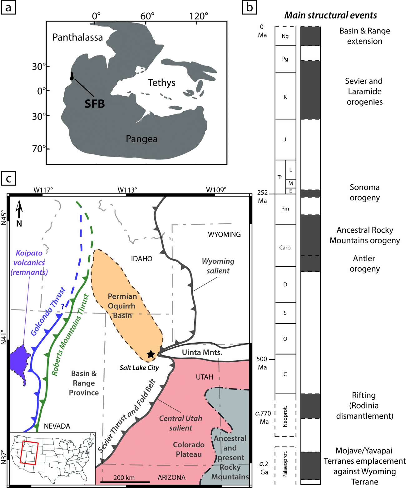
Figure 1. (a) Early Triassic location of the Sonoma Foreland Basin (SFB; after Brayard et al. Reference Brayard, Bylund, Jenks, Stephen, Olivier, Escarguel, Fara and Vennin2013). (b) Simplified chronostratigraphy of the succession of structuring events in the studied area since Palaeoproterozoic time (after Oldow et al. Reference Oldow, Bally, Avé Lallemant, Leeman, Bally and Palmer1989; Whitmeyer & Karlstrom, Reference Whitmeyer and Karlstrom2007; Dickinson, Reference Dickinson2013). (c) Simplified map of the study area with location of the main structural elements discussed and mentioned in this work (after Bond et al. Reference Bond, Christie-Blick, Kominz and Devlin1985; Walker, Reference Walker1985; Dickinson, Reference Dickinson2004, Reference Dickinson2006, Reference Dickinson2013; Vetz, Reference Vetz2011; Yonkee & Weil, Reference Yonkee and Weil2015).
Foreland sedimentary basins are generally considered as passive systems resulting from the flexural subsidence of the elastic lithosphere in response to crustal thickening and sediment loading (e.g. DeCelles & Giles, Reference DeCelles and Giles1996; Allen & Allen, Reference Allen and Allen2005). If the flexural isostatic model is a reasonable first-order explanation for the overall shape of foreland basins, sediment thickness variations and peculiar stratigraphic successions involve a differential local subsidence. In order to decipher such potential mechanisms at the origin of the SFB structuring and sedimentary record variations, we use a multidisciplinary approach. We perform a subsidence analysis of the basin within a high-resolution biostratigraphically controlled timeframe from the Permian–Triassic unconformity (PTU) up until late Smithian time (a c. 1.3 Ma long interval; the Smithian is the third substage of the Early Triassic). This allows us to characterize the basin infill in relation to the emplacement of the Golconda Allochthon during the Sonoma orogeny. We also provide new evidence indicating that the studied area is a foreland basin. Using a complementary backstripping approach and numerical models we discuss the main factors controlling the subsidence variations observed in the SFB, including the impact of lithospheric and rheological features, on basement partitioning and sedimentation.
2. Geological setting
2.a. Brief geological history of the study area
The Sonoma Foreland Basin lies within a region of the North American continent showing a very long and complex tectonosedimentary history starting during Proterozoic time and still active today (e.g. Dickinson, Reference Dickinson2013). The first documented structuring of the region dates back to the Palaeoproterozoic period when Mojave and Yavapai terranes were emplaced against the Archean Wyoming craton (Fig. 1b; Whitmeyer & Karlstrom, Reference Whitmeyer and Karlstrom2007; Lund et al. Reference Lund, Box, Holm-Denoma, San Juan, Blakely, Saltus, Anderson and Dewitt2015). This event generated multiple crustal fault zones along which later reactivations were possible with deformational episodes (Oldow et al. Reference Oldow, Bally, Avé Lallemant, Leeman, Bally and Palmer1989; Dickerson, Reference Dickerson2003). At least two rifting events took place in this region during subsequent Proterozoic times (Burchfiel & Davis, Reference Burchfiel and Davis1975; Oldow et al. Reference Oldow, Bally, Avé Lallemant, Leeman, Bally and Palmer1989), the most recent being during Neoproterozoic time (c. 770 Ma) and linked to the fragmentation of the supercontinent Rodinia (Fig. 1b; Dickinson, Reference Dickinson2006). The long period of tectonic quiescence following the formation of this passive margin lasted until Late Devonian time (c. 380 Ma) and corresponds to the deposition of a thick sedimentary prism formerly known as the ‘Cordilleran Miogeocline’ (Clark, Reference Clark1957; Paull & Paull, Reference Paull and Paull1991; Dickinson, Reference Dickinson2006, Reference Dickinson2013).
Starting during Late Devonian time and lasting until late Early Carboniferous time, the Antler orogeny marks the beginning of a period of nearly continuous structural events that are still active today (Fig. 1b). The Antler orogeny was caused by the convergence and accretion of exotic island-arcs against the western margin of the North American Plate. This orogeny is characterized by the emplacement of a large obducted accretionary prism located in Central Nevada today (i.e. Roberts Mountains Thrust, Fig. 1c; Burchfiel & Davis, Reference Burchfiel and Davis1975; Speed & Sleep, Reference Speed and Sleep1982; Speed & Silberling, Reference Speed and Silberling1989; Burchfiel & Royden, Reference Burchfiel and Royden1991). The Roberts Mountains Allochthon led to the formation of the N–S-trending westwards-dipping Antler Foreland Basin (Speed & Sleep, Reference Speed and Sleep1982; Burchfiel & Royden, Reference Burchfiel and Royden1991; Blakey, Reference Blakey2008; Ingersoll, Reference Ingersoll2008; Dickinson, Reference Dickinson2004, Reference Dickinson2006, Reference Dickinson2013).
Soon after the Antler orogeny the Ancestral Rocky Mountains (ARM) orogeny occurred on the eastern part of the region (Fig. 1c), ranging over Early Carboniferous to early–middle Permian time (c. 350–270 Ma; Fig. 1b). This mountain-building event resulted from a succession of crustal uplifts because of important long-range intracratonic deformations. There, transtensional and transpressional constraints occurred along with lithospheric buckling as a response to the Laurentia–Gondwana continental collision (Kluth & Coney, Reference Kluth and Coney1981; Ye et al. Reference Ye, Royden, Burchfiel and Schuepbach1996; Geslin, Reference Geslin1998; Dickerson, Reference Dickerson2003; Dickinson, Reference Dickinson2006, Reference Dickinson2013; Blakey, Reference Blakey2008). The resulting chain probably showed a marked topographic relief, some of which could have persisted until Early Triassic time (Kluth & Coney, Reference Kluth and Coney1981; Blakey, Reference Blakey2008). Most of these crustal uplifts were emplaced according to lithospheric weaknesses inherited from the Proterozoic structural events (Kluth & Coney, Reference Kluth and Coney1981; Dickerson, Reference Dickerson2003).
Many sedimentary basins formed during the Carboniferous–Permian interval (Dickerson, Reference Dickerson2003). For instance, the Permian Oquirrh Basin (Fig. 1c) probably resulted from the complex interplay between intracratonic deformations to the east and the reactivation of Antler faults to the west (Geslin Reference Geslin1998: fig. 12; Trexler & Nitchman, Reference Trexler and Nitchman1990; Dickerson, Reference Dickerson2003; Blakey, Reference Blakey2008). This highly subsiding basin recorded up to 6 km of marine strata (Walker, Reference Walker1985; Yonkee & Weil, Reference Yonkee and Weil2015).
Similarly to the Antler orogeny, the Sonoma orogeny is the result of the eastwards migration and accretion of exotic island-arc systems belonging to the Sonomia microplate onto the North American Plate around the Permian–Triassic boundary (Burchfiel & Davis, Reference Burchfiel and Davis1975; Speed & Silberling, Reference Speed and Silberling1989; Dickinson, Reference Dickinson2006, Reference Dickinson2013; Blakey, Reference Blakey2008; Ingersoll, Reference Ingersoll2008). The Sonoma orogeny is characterized by the thrusting of an accretionary prism above continental crust, known as the Golconda Allochthon, and emplaced in the same area as the older Roberts Mountains Allochthon (Fig. 1c). The Golconda Allochthon is thought to have initiated the formation of a foreland basin – the Sonoma Foreland Basin (Dickinson, Reference Dickinson2006, Reference Dickinson2013; Blakey, Reference Blakey2008; Ingersoll, Reference Ingersoll2008) – which recorded sediments deposited during Early Triassic time. However, field evidence pointing towards the location and extension of the Golconda Allochthon is restricted to only a few remnants (e.g. ‘Koipato volcanics’) near the southern part of the basin, which are presently located in Central Nevada (Fig. 1c; Snyder & Brueckner, Reference Snyder, Brueckner and Stevens1983; Walker, Reference Walker1985; Schweickert & Lahren, Reference Schweickert and Lahren1987; Oldow et al. Reference Oldow, Bally, Avé Lallemant, Leeman, Bally and Palmer1989; Dickinson, Reference Dickinson2006, Reference Dickinson2013; Blakey, Reference Blakey2008; Ingersoll, Reference Ingersoll2008). Remnants of the Golconda Allochthon, if any, are yet to be found in the northern part of the basin, especially in Idaho (Schweickert & Lahren, Reference Schweickert and Lahren1987; Oldow et al. Reference Oldow, Bally, Avé Lallemant, Leeman, Bally and Palmer1989). This allochthon is sealed in present-day Nevada by the rhyolitic Koipato Formation volcanism, presumably emplaced by the end of the Sonoma orogeny (Vetz, Reference Vetz2011). A minimum age of Anisian (Middle Triassic) can be given to this volcanic formation using geochronology (Vetz, Reference Vetz2011) and due to the occurrence of Anisian ammonites in the unconformably overlying sedimentary series (Nichols & Silberling, Reference Nichols and Silberling1977; Bucher, Reference Bucher1988; Vetz, Reference Vetz2011). The potential presence of older ammonoid faunas is not to be discarded.
The following Sevier orogeny is of Early Cretaceous – Eocene age (c. 140–50 Ma; Fig. 1b) and it originated from the subduction of the Farallon Plate under the North American continental plate (Burchfiel & Davis, Reference Burchfiel and Davis1975; Dickinson, Reference Dickinson2006, Reference Dickinson2013). E–W-directed compressive constraints resulted in the formation of a large Sevier thrust-and-fold belt which is still present today and constitutes the eastern border of the Great Basin (Fig. 1c; Dickinson, Reference Dickinson2006, Reference Dickinson2013; Yonkee & Weil, Reference Yonkee and Weil2010; Yonkee et al. Reference Yonkee, Dehler, Link, Balgord, Keeley, Hayes, Wells, Fanning and Johnston2014). This thrust-and-fold belt is however not homogeneous along its N–S-trending front, and displays two convex-to-the-foreland ‘salients’ (Fig. 2) with varying estimated tectonic shortening and eastwards displacement of terrains reaching up to 140 km (DeCelles & Coogan, Reference DeCelles and Coogan2006; Schelling et al. Reference Schelling, Strickland, Johnson, Vrona, Willis, Hylland, Clark and Chidsey2007; Dickinson, Reference Dickinson2006, Reference Dickinson2013; Yonkee & Weil, Reference Yonkee and Weil2010, Reference Yonkee and Weil2015; Yonkee et al. Reference Yonkee, Dehler, Link, Balgord, Keeley, Hayes, Wells, Fanning and Johnston2014). These Wyoming and Central Utah salients are separated by a conspicuous recess formed by a lateral ramp and located west of the Uinta Mountains (Figs 1c, 2). Its formation results from inherited features of the basement (see Section 4.c; e.g. Lawton, Boyer & Schmitt, Reference Lawton, Boyer and Schmitt1994; Mukul & Mitra, Reference Mukul and Mitra1998; Paulsen & Marshak, Reference Paulsen and Marshak1999; Wilkerson, Apotria & Farid, Reference Wilkerson, Apotria and Farid2002).
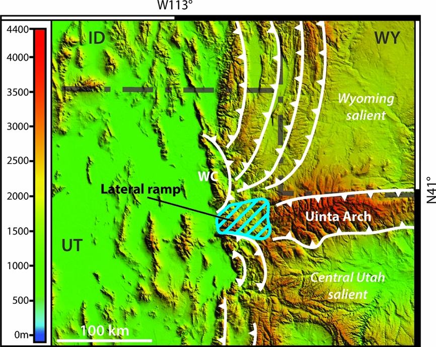
Figure 2. Topographic map of the central part of current-day Sevier thrust-and-fold belt with accentuation of the Wyoming and Central Utah salients thrusts. A lateral ramp is present between the two salients (after Paulsen & Marshak, Reference Paulsen and Marshak1999).
Also during Early Cretaceous – Eocene time, the eastern Laramide orogeny reactivated basal crustal uplifts set during the Ancestral Rocky Mountains orogeny. This led to the formation of the modern-day Rocky Mountains which overlapped older structures in the Colorado Plateau (Fig. 1b, c; Oldow et al. Reference Oldow, Bally, Avé Lallemant, Leeman, Bally and Palmer1989; Ye et al. Reference Ye, Royden, Burchfiel and Schuepbach1996; Dickinson, pers. comm. 2015).
Finally, the Basin and Range extension of the entire region started during Neogene time (c. 20 Ma; Fig. 1b) and is still active today (Oldow et al. Reference Oldow, Bally, Avé Lallemant, Leeman, Bally and Palmer1989; DeCelles & Coogan, Reference DeCelles and Coogan2006; Dickinson, Reference Dickinson2002, Reference Dickinson2006, Reference Dickinson2013). This extension is the result of internal forces (Kreemer & Hammond, Reference Kreemer and Hammond2007) that generated transtensional stresses and pure shear (Parsons, Thompson & Sleep, Reference Parsons, Thompson and Sleep1994; Gans & Bohrson, Reference Gans and Bohrson1998; Dickinson, Reference Dickinson2002, Reference Dickinson2006). However, the origin of these extensional constraints is still being discussed. Several possible mechanisms have been proposed, including: (1) a mantellic ‘wide rift-like’ process with ascent and underplating of mantellic material leading to thermal lamination of the lithosphere (Lachenbruch & Morgan, Reference Lachenbruch and Morgan1990; Parsons, Thompson & Sleep, Reference Parsons, Thompson and Sleep1994, Gans & Bohrson, Reference Gans and Bohrson1998); or (2) a mechanical origin with the extension occurring in a late orogenic context, due to the instability and gravity collapse of the thickened lithospheric crust present in Nevada and westernmost Utah (Fletcher & Hallet Reference Fletcher and Hallet1983; Malavieille, Reference Malavieille1993; Zandt, Myers & Wallace, Reference Zandt, Myers and Wallace1995). Nevertheless, the easternmost borders of the basin (e.g. Colorado Plateau or Uinta Mountains) are not affected by these displacements (Fig. 1c; Dickinson, Reference Dickinson2006, Reference Dickinson2013). It is also worth noting that this extension reactivates in inversion some of the thrust faults created during the Sevier orogeny (Coney, Reference Coney1987; Dickinson, Reference Dickinson2006, Reference Dickinson2013).
2.b. Sedimentary record of the Sonoma Foreland Basin
Here we focus on the Early Triassic sedimentary record of the Sonoma Foreland Basin (Figs 3a, 4). The stratigraphic succession displays marked spatial differences in thickness and in dominant lithologies (Fig. 4). The sedimentary record is considered as almost continuous throughout the basin, with local erosion surfaces being under the temporal resolution of ammonoid biozones for this Early Triassic interval (e.g. Olivier et al. Reference Olivier, Brayard, Fara, Bylund, Jenks, Vennin, Stephen and Escarguel2014, Reference Olivier, Brayard, Vennin, Escarguel, Fara, Bylund, Jenks, Caravaca and Stephen2016; Vennin et al. Reference Vennin, Olivier, Brayard, Bour, Thomazo, Escarguel, Fara, Bylund, Jenks, Stephen and Hofmann2015). In its southern part (Figs 3a, 4), the basin is mainly filled with transitional continental to marine coarse sandstones to conglomerates known as ‘red beds’ of the Moenkopi Group (Fig. 5a–c, e; sensu Lucas, Krainer & Milner, Reference Lucas, Krainer and Milner2007; Brayard et al. Reference Brayard, Bylund, Jenks, Stephen, Olivier, Escarguel, Fara and Vennin2013). At the top of the Moenkopi Group, metric-scale beds of intertidal microbial limestones can be observed (Figs 3a, 4, 5e; Brayard et al. Reference Brayard, Bylund, Jenks, Stephen, Olivier, Escarguel, Fara and Vennin2013; Vennin et al. Reference Vennin, Olivier, Brayard, Bour, Thomazo, Escarguel, Fara, Bylund, Jenks, Stephen and Hofmann2015; Olivier et al. Reference Olivier, Brayard, Vennin, Escarguel, Fara, Bylund, Jenks, Caravaca and Stephen2016). The upper part of the sedimentary pile is characterized by open-marine bioclastic limestones (locally shales) of the Thaynes Group (Figs 3a, 4, 5d, f; sensu Lucas, Krainer & Milner, Reference Lucas, Krainer and Milner2007), marking the maximum flooding of the Smithian third-order transgression (Embry, Reference Embry1997; Vennin et al. Reference Vennin, Olivier, Brayard, Bour, Thomazo, Escarguel, Fara, Bylund, Jenks, Stephen and Hofmann2015). This flooding event is characterized by the presence of the ammonoid genus Anasibirites (Figs 3a, 4; Lucas, Krainer & Milner, Reference Lucas, Krainer and Milner2007; Brayard et al. Reference Brayard, Bylund, Jenks, Stephen, Olivier, Escarguel, Fara and Vennin2013; Jattiot et al. Reference Jattiot, Bucher, Brayard, Monnet, Jenks and Hautmann2015, in press). In the northern part of the basin (Figs 3a, 4) the sedimentary record differs at its base by the presence of the Dinwoody and Woodside formations, characterized by fine marine siltstones (Figs 3a, 4, 5g; Kummel, Reference Kummel1954, Reference Kummel and Ladd1957; Sadler, Reference Sadler1981; Paull & Paull, Reference Paull and Paull1991). Above these formations, the sedimentary record resembles that observed in the southern part and corresponds to the open-marine bioclastic limestones and shales of the Thaynes Group (Figs 3a, 4, 5d, h). A basin-scale synthetic facies analysis with associated depositional environments and estimations of the palaeobathymetries can be found in online Supplementary Table S1 (available at http://journals.cambridge.org/geo).
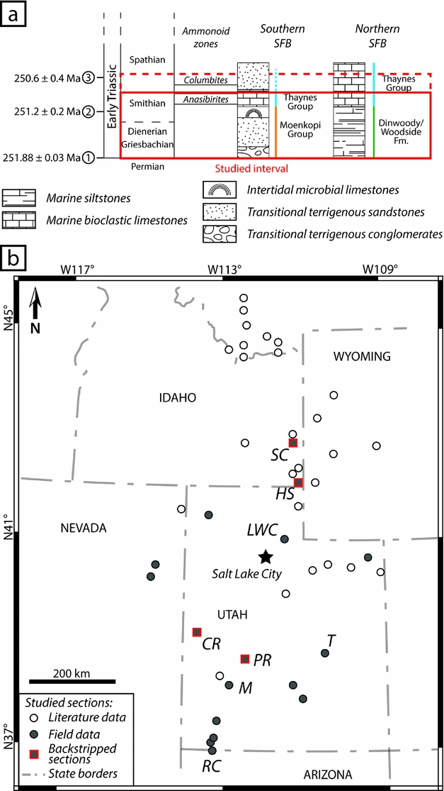
Figure 3. (a) Simplified litho- and chronostratigraphic subdivisions of the Early Triassic Sonoma Foreland Basin (SFB). This study encompasses the PTU-Smithian interval, with Spathian complement for the subsidence analysis. Main ammonoid markers used in this study are the Anasibirites beds and the Columbites beds. Radiometric ages: (1) from Burgess, Bowring & Shen (Reference Burgess, Bowring and Shen2014); (2) and (3) from Galfetti et al. (Reference Galfetti, Bucher, Ovtcharova, Schaltegger, Brayard, Brühwiler, Goudemand, Weissert, Hochuli, Cordey and Guodun2007). (b) State map of the study area showing current location of the 43 studied sections, from both literature data (open circles) and field data (grey circles). Complete GPS coordinates and references are given in online Supplementary Table S2. Red outlines highlight the sections used for the subsidence analysis, and selected for their completeness, temporal resolution and spatial distribution. Sections detailed in Figure 4: SC: Sheep Creek; HS: Hot Springs; LWC: Lower Weber Canyon; CR: Confusion Range; T: Torrey area; PR: Pahvant Range; M: Minersville; RC: Rock Canyon.

Figure 4. Biostratigraphic correlation based on the Anasibirites and Columbites beds observed in 8 of the 43 studied sections, illustrating the discrepancy in sedimentary thickness between the southern and northern parts of the Sonoma Foreland Basin (with simplified lithology). Base of the sections corresponds to the regionally recognized Permian–Triassic unconformity (Brayard et al. Reference Brayard, Bylund, Jenks, Stephen, Olivier, Escarguel, Fara and Vennin2013).
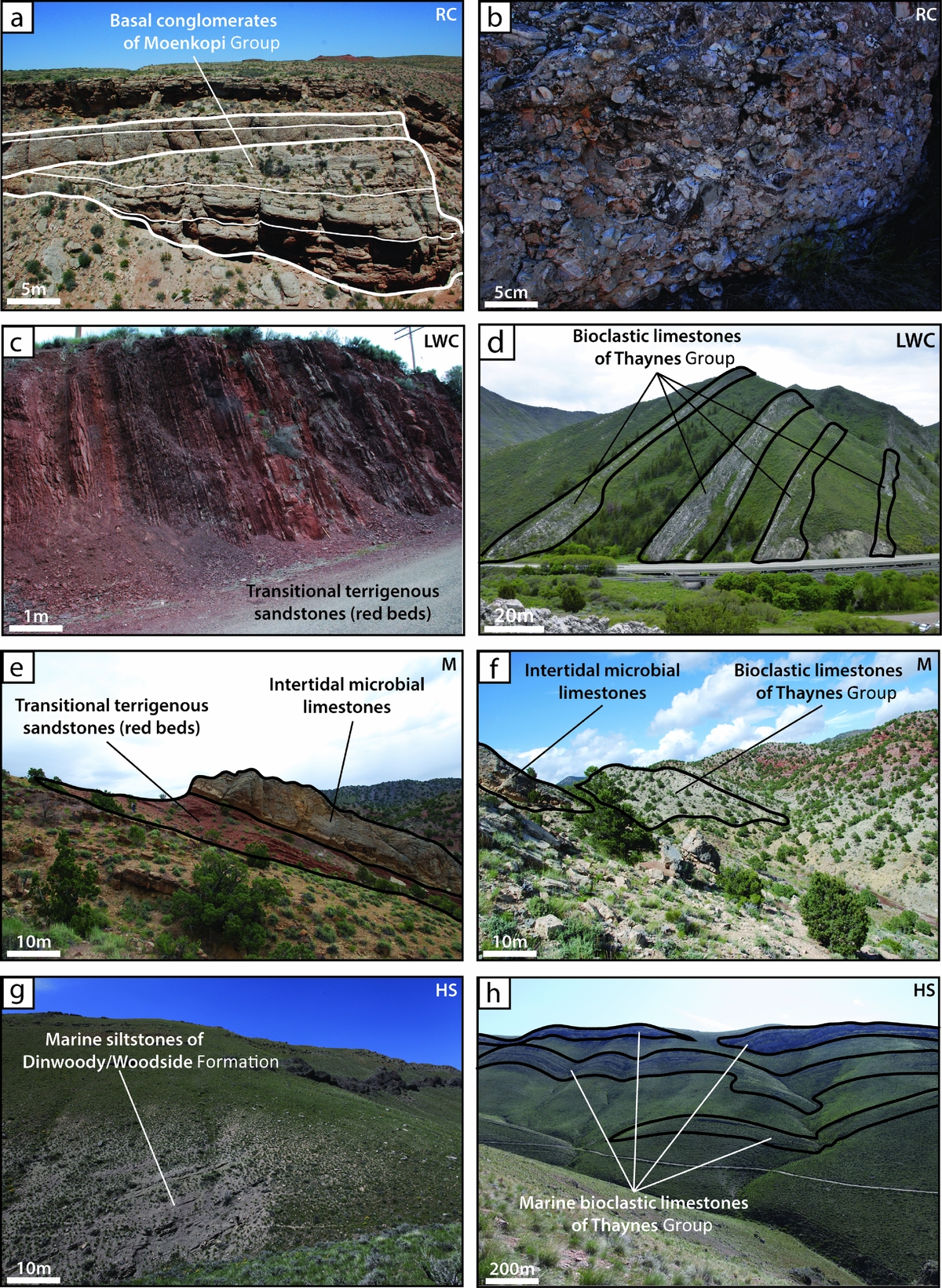
Figure 5. Photographs of different outcrops in the SFB, showing variations in dominant lithologies and sedimentary thicknesses encountered throughout the basin. (a) Panorama of Rock Canyon (RC) outcrop, showing the plurimetric beds of conglomerates from the basal Moenkopi Group. (b) Detail photograph of the conglomerate from Rock Canyon. (c) Photograph of the terrigenous red beds of the Moenkopi Group at Lower Weber Canyon (LWC). (d) Panorama of the limestones beds of the Thaynes Group limestones at Lower Weber Canyon. (e) Panorama of the Moenkopi Group at Minersville (M), showing succession of terrigenous red beds and microbial limestones. (f) Panorama of the transition between Moenkopi and Thaynes Group showing succession of microbial limestones and bioclastic limestones at Minersville. (g) Photograph of the marine siltstones of the Dinwoody and Woodside Formation at Hot Springs (HS). (h) Panorama of the Hot Springs section, showing succession of limestone levels of the Thaynes Group bioclastic limestones.
3. Dataset and methods
3.a. Dataset
We compiled a comprehensive sedimentary and biostratigraphic dataset for the Early Triassic outcrops in the Sonoma Foreland Basin, including previously published works (e.g. Kummel, Reference Kummel1954, Reference Kummel and Ladd1957; Paull & Paull, Reference Paull and Paull1991; Goodspeed & Lucas, Reference Goodspeed and Lucas2007; Heckert et al. Reference Heckert, Chure, Voris, Harrison, Thomson, Berg, Ressetar and Birgenheier2015) together with new field data (Fig. 3b). We selected 43 biostratigraphically correlated sections documenting different parts of the basin in order to estimate the thickness (at the metre scale) of the sedimentary deposits (GPS coordinates and main characteristics of each section are provided in online Supplementary Table S2). The 43 studied sections correspond to the Early Triassic interval. The base of this interval is defined by a major regional PTU (Brayard et al. Reference Brayard, Bylund, Jenks, Stephen, Olivier, Escarguel, Fara and Vennin2013). Its upper end is determined by the Anasibirites beds or the uppermost part of the Owenites beds as a surrogate, which are the main biostratigraphic markers of the end-Smithian (Figs 3a, 4; Brayard et al. Reference Brayard, Bylund, Jenks, Stephen, Olivier, Escarguel, Fara and Vennin2013; Jattiot et al. Reference Jattiot, Bucher, Brayard, Monnet, Jenks and Hautmann2015). Eleven sections were delimited using a high-resolution ammonoid zonation (e.g. sections in Fig. 4; Brayard et al. Reference Brayard, Bylund, Jenks, Stephen, Olivier, Escarguel, Fara and Vennin2013). We conservatively used only minimum thickness values for the 32 sections taken from the literature because they are not always based on homogeneous sedimentary and biostratigraphical data (online Supplementary Table S2). For completeness of the subsidence analysis, we included when possible thickness data available for the lower part of the Spathian (fourth substage of the Early Triassic), the Columbites beds marking in this case the end of the studied interval (Fig. 3a).
3.b. Methods
3.b.1. Palinspastic reconstructions using retrodeformations
Post-Triassic times in the Sonoma Foreland Basin are characterized by important tectonic compressive and later extensive deformations. These successive deformations are mostly represented in the basin by the complex and heterogeneous Sevier thrust-and-fold belt. The palaeogeographic configuration of the Sonoma Foreland Basin was therefore different compared to the modern configuration. In order to resolve this issue, we performed a palinspastic reconstruction to estimate the Early Triassic palaeogeography of this basin.
Retrodeformations of observed structural features affecting the Triassic series were applied to several regional cross-sections using literature data (e.g. DeCelles & Coogan, Reference DeCelles and Coogan2006; Yonkee & Weil, Reference Yonkee and Weil2010; Fig. 6). This method consists of the horizontalization of a selected layer (here the Triassic series) by virtually inverting all the structural features observed in the section between a fixed reference point named the ‘pin line’ and a mobile reference point named the ‘loose line’ (Fig. 6; see Groshong, Reference Groshong2006 for details). In the two regional cross-sections of the Sevier thrust-and-fold belt illustrated in Figure 6, most structural features are thrust complexes; horizontalization therefore mainly consists of retrodeformation of the displacements along thrust planes. Finally, balanced cross-sections represent a good approximation of the geomorphological setting by the time of deposition. Based on this method, the direction and value of the estimated tectonic transport (ETT) underwent by the terrains can also be calculated (e.g. c. 140 km and c. 60 km for the cross-sections a and b in Fig. 6, respectively).
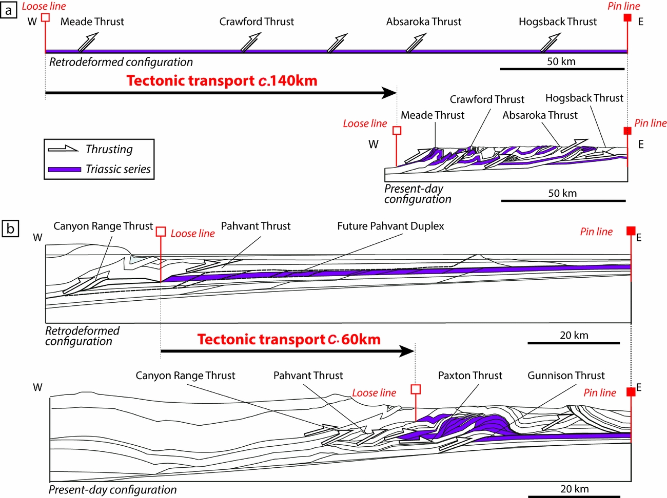
Figure 6. Present-day and retrodeformed (for the PTU-Smithian interval) configurations for two regional cross-sections in the (a) northern and (b) southern parts of the Sonoma Foreland Basin, illustrating the method used for palinspastic reconstruction (after Groshong, Reference Groshong2006). Balanced cross-sections adapted from (a) Yonkee & Weil (Reference Yonkee and Weil2010) and (b) DeCelles & Coogan (Reference DeCelles and Coogan2006) illustrate the retrodeformation process used to estimate the value of the tectonic transport, and therefore the approximate original location of the sections during the studied interval. Triassic series (highlighted layers) are used as the basis for the retrodeformation process and are horizontalized between the designated Pin and Loose lines (see text for details). The two cross-sections are located in Figure 7.
Due to the complex nature of the Sevier thrust-and-fold belt resulting from the inherited structure and thickness pattern of the pre-deformation basins (Paulsen & Marshak, Reference Paulsen and Marshak1999), and also the westwards focalization of the subsequent Basin and Range extension, ETT was spatially heterogeneous between Wyoming and Central Utah salients (Mukul & Mitra, Reference Mukul and Mitra1998; DeCelles & Coogan, Reference DeCelles and Coogan2006; Schelling et al. Reference Schelling, Strickland, Johnson, Vrona, Willis, Hylland, Clark and Chidsey2007; Yonkee & Weil, Reference Yonkee and Weil2010; Yonkee et al. Reference Yonkee, Dehler, Link, Balgord, Keeley, Hayes, Wells, Fanning and Johnston2014). We therefore defined seven sectors within our study area (sectors 1–7 in Fig. 7). These sectors were delimited based on similar ETT values (Table 1; Fig. 7). These values were determined from data available in the literature (references in Table 1) and checked with the retrodeformation of regional cross-sections taken from geological maps (cross-sections in Fig. 6).
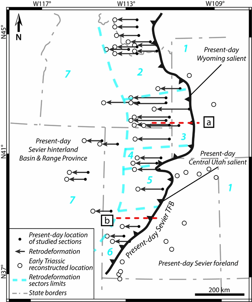
Figure 7. Map representing the present-day location of the studied sections (dots) and their reconstructed position (open circles) obtained after retrodeformation. Positions of balanced cross-sections (a) and (b) illustrated in Figure 6 are also indicated. The present-day Sevier Thrust-and-Fold Belt (TFB; after Yonkee et al. Reference Yonkee, Dehler, Link, Balgord, Keeley, Hayes, Wells, Fanning and Johnston2014) is the main structural element responsible for tectonic transport during post-Triassic times. Black arrows represent the retrodeformation values applied from the present-day location of the studied sections. Seven sectors of similar estimated tectonic transport are delimited by dashed lines (see Table 1). Sector 1: Sevier foreland; Sector 2: Wyoming salient, northern part; Sector 3: Wyoming salient, central part; Sector 4: Wyoming salient, southern part; Sector 5: Central Utah salient, northern part; Sector 6: Central Utah salient, southern part; Sector 7: Sevier hinterland.
Table 1. Estimated tectonic transport values used for palinspastic reconstructions of each sectors defined within the SFB, and associated references.

3.b.2. Subsidence analysis and backstripping
Subsidence analysis quantifies the vertical movements underwent by a given sedimentary depositional surface through a graphic representation, by tracking the subsidence and uplift history of said surface (Van Hinte, Reference Van Hinte1978). This history is reconstructed based on sedimentary thickness, lithology, palaeo-sea level, palaeobathymetry and age data. This analysis also accounts for the mechanical compaction underwent by the sediments. The resulting curve provides a view of the total subsidence history for a given stratigraphic column (Van Hinte, Reference Van Hinte1978; Allen & Allen, Reference Allen and Allen2005). Steckler & Watts (Reference Steckler and Watts1978) showed that the local isostatic effect exerted by the sedimentary load can be removed. This ‘backstripping’ method can therefore help to characterize the tectonic subsidence only, as if the basin has been filled by air only and not by water and/or sediment during its history (Steckler & Watts, Reference Steckler and Watts1978; Xie & Heller, Reference Xie and Heller2009). Backstripping is also used to restore the initial thickness of a sedimentary column (Angevine, Heller & Paola, Reference Angevine, Heller and Paola1990; Allen & Allen, Reference Allen and Allen2005). Lithological compositions and palaeobathymetries have been checked using facies analysis (online Supplementary Table S1) or literature data (see analysed sections in Fig. 3b and online Supplementary Table S2). Porosity was quantified by comparison with experimental data (e.g. Van Hinte, Reference Van Hinte1978; Sclater & Christie, Reference Sclater and Christie1980) and represents an important proxy for compaction analysis. Additionally, Chevalier et al. (Reference Chevalier, Guiraud, Garcia, Dommergues, Quesne, Allemand and Dumont2003) and Lachkar et al. (Reference Lachkar, Guiraud, El Harfi, Dommergues, Dera and Durlet2009) showed that a highly resolved biostratigraphic control is useful to define and quantify variations in subsidence at a fine spatio-temporal scale as it yields accurate subsidence rates. For the Early Triassic Sonoma Foreland Basin, the high-resolution ammonoid zonation by Brayard et al. (Reference Brayard, Bylund, Jenks, Stephen, Olivier, Escarguel, Fara and Vennin2013) serves as the main timeframe. Complementary absolute time lines were obtained from radiometric ages published from coeval beds in South China (Galfetti et al. Reference Galfetti, Bucher, Ovtcharova, Schaltegger, Brayard, Brühwiler, Goudemand, Weissert, Hochuli, Cordey and Guodun2007; Burgess, Bowring & Shen, Reference Burgess, Bowring and Shen2014), whereas the duration of the studied intervals was interpolated from ammonoid biozone duration (after Brühwiler et al. Reference Brühwiler, Bucher, Brayard and Goudemand2010 and Ware et al. Reference Ware, Bucher, Brayard, Schneebeli-Hermann and Brühwiler2015). Palaeo-sea level curve is based on data from Haq, Hardenbol & Vail (Reference Haq, Hardenbol, Vail, Wilgus, Hastings, Posamentier, Wagoner, Ross and Kendall1988), providing a quantitative representation of the reconstructed Early Triassic sea level.
We chose to not use the flexural backstripping method (Allen & Allen, Reference Allen and Allen2005) due to the lack of appropriate data needed for such model (e.g. flexural rigidity data, regional distribution of the sedimentary load). Instead, we calculated the total and tectonic subsidence curves using the one-dimensional (1D) local isostatic approach of Steckler & Watts (Reference Steckler and Watts1978). In addition, this method emphasizes the tectonic subsidence as ‘a way of normalizing subsidence in different basins that have undergone very different sedimentation histories’ (Xie & Heller, Reference Xie and Heller2009). Our results for the tectonic subsidence history in the SFB can therefore be compared to the compilation of Xie & Heller (Reference Xie and Heller2009). Subsidence analyses were performed on four sections (Fig. 3b) using the OSXBackstrip software performing 1D Airy backstripping (after Watts, Reference Watts2001; Allen & Allen, Reference Allen and Allen2005; available at: http://www.ux.uis.no/~nestor/work/programs.html). These sections were selected for their completeness (a complete and continuous sedimentary succession is reported from the PTU to at least lower Spathian stratigraphy), for the presence of biostratigraphic markers (ammonoid beds) and for their repartition within the SFB (representative of both the northern and southern areas). A complete set of initial parameters and detailed results of the subsidence analysis for each of the four sections are reported in online Supplementary Material S1.
This analysis bears limitations as some errors may arise from uncertainties around the data used for the subsidence analysis (Chevalier et al. Reference Chevalier, Guiraud, Garcia, Dommergues, Quesne, Allemand and Dumont2003; Xie & Heller, Reference Xie and Heller2009): (1) accuracy of the measurement and report of the sedimentary thickness; (2) backstripping calculation; (3) palaeo-bathymetry estimations; and (4) age control. Regarding the accuracy of the sediment thickness, all selected sections have been measured at a centimetric scale. Errors on measurements are therefore rather low, i.e. ±2% of the total thickness. In the backstripping analysis, variables used for the calculation of the burial compaction are: thickness; the initial porosity of the sediment; and the lithological constant of corresponding lithologies. The latter two parameters are determined by comparison with experimental data (e.g. Van Hinte, Reference Van Hinte1978; Sclater & Christie, Reference Sclater and Christie1980). Error on sediment decompaction is therefore estimated to be low (c. ±5%). Palaeobathymetry is hard to determine because of the paucity of discriminating indicators. We hypothesize that errors on depth estimations are about ±10%. For age control, we used a compilation of biostratigraphic and radiochronological data, leading to a detailed timeframe with a maximum error of around 60 ka (Brühwiler et al. Reference Brühwiler, Bucher, Brayard and Goudemand2010).
3.b.3. Spatial distribution of sedimentary thickness
PTU-Smithian sedimentary thicknesses and their respective location within the SFB were integrated in Global Mapper v.16.2.3 GIS software (available at http://www.bluemarblegeo.com/products/global-mapper.php) to generate an isopach map by creating a 3D triangulated grid projection of thicknesses (online Supplementary Figure S1).
3.b.4. Lithospheric heterogeneity of the basement
To explore the nature of the SFB basement, a terrane map was constructed using previous published maps by Yonkee et al. (Reference Yonkee, Dehler, Link, Balgord, Keeley, Hayes, Wells, Fanning and Johnston2014), Yonkee & Weil (Reference Yonkee and Weil2015) and Lund et al. (Reference Lund, Box, Holm-Denoma, San Juan, Blakely, Saltus, Anderson and Dewitt2015). In addition, we analysed several types of geophysical data: a raw regional Bouguer gravity anomaly map (Kucks, Reference Kucks1999); an aeromagnetic anomaly map from Bankey et al. (Reference Bankey, Cuevas, Daniels, Finn, Hernandez, Hill, Kucks, Miles, Pilkington, Roberts, Roest, Rystrom, Shearer, Snyder, Sweeney, Velez, Phillips and Ravat2002); and literature data (e.g. Gilbert, Velasco & Zandt, Reference Gilbert, Velasco and Zandt2007). We also used published U/Pb radiochronological data to assess an age for each basement terrane defined in the basin (Foster et al. Reference Foster, Mueller, Mogk, Wooden and Vogl2006; Fan et al. Reference Fan, DeCelles, Gehrels, Dettman, Quade and Peyton2011; Mueller et al. Reference Mueller, Wooden, Mogk and Foster2011; Nelson, Hart & Frost, Reference Nelson, Hart and Frost2011; Strickland, Miller & Wooden, Reference Strickland, Miller and Wooden2011). It is worth noting that Precambrian crystalline basements, lying under detachments and décollements responsible for nucleation of thrusting, are not affected by these ‘thin-skin’ thrust-induced displacements (DeCelles & Coogan, Reference DeCelles and Coogan2006; Schelling et al. Reference Schelling, Strickland, Johnson, Vrona, Willis, Hylland, Clark and Chidsey2007; Yonkee & Weil, Reference Yonkee and Weil2010).
3.b.5. Numerical model
The flexural response of the SFB basement has been simulated using a 2D plane stress flexural model solved with a finite element method code written in Matlab®. This approach has been successfully used to model lithospheric deformation due to topographic and mantle loads (Le Pourhiet & Saleeby, Reference Le Pourhiet and Saleeby2013) and ice loads (Moreau et al. Reference Moreau, Le Pourhiet, Huuse, Gibbard and Grappe2015). First, a model of the basin is made using field-based and literature data to characterize and quantify the flexural response of the modelled SFB basement. Three additional models are then proposed to test different scenarios regarding possible mechanisms controlling the flexure of the SFB basement.
4. Results
We first reconstructed the SFB palaeogeography and used lithological and stratigraphical analyses to constrain the spatial distribution of the sedimentary record across the basin. This approach provides estimations of subsidence rates in the SFB. Secondly, we identified and characterized the terranes that compose the SFB basement using geophysical and cartographic data, as well as previously published ages. We then reconstructed the morphology of the Golconda Allochthon in relation to the heritage of the basin. Finally, a 2D model is proposed to quantify the flexural behaviour of the basin.
4.a. Lithological and stratigraphical analyses
Previous palaeogeographic reconstructions of the SFB did not take tectonic events and the ensuing displacements into account (e.g. Paull & Paull, Reference Paull and Paull1993). The palinspastic map of the basin with the initial locations of the studied sections is shown on Figure 7. For the first time post-Triassic displacements were accounted for, including: (1) the Sevier orogeny (Cretaceous–Eocene) and the associated regional shortening due to the setting of a thrust-and-fold belt (e.g. Yonkee & Weil, Reference Yonkee and Weil2010); and (2) the later Neogene – present-day extension linked to the Basin and Range province (e.g. Yonkee et al. Reference Yonkee, Dehler, Link, Balgord, Keeley, Hayes, Wells, Fanning and Johnston2014).
Based on the palinspastic map, we constructed a palaeogeographic isopach map of the SFB (Fig. 8). The isopach map shows that the distribution of the sedimentary thickness for the PTU-Smithian interval is heterogeneous within the basin, showing a thicker succession in the northern than in the southern part. In the southern part, the thickness gradually varies along a roughly NW–SE-aligned transect, showing low thicknesses over a large surface (c. 500 km from east to west). The thickness ranges from a few tenths of metres in south and SE Utah, up to 250 m around Salt Lake City. The westernmost area (NE Nevada) is also characterized by low thicknesses (˂100 m thick). Conversely, the northern part of the basin exhibits a marked transition with thickness values broadly increasing from east to west. The easternmost area of the northern part (west Wyoming) shows sedimentary thicknesses similar to that of the southern part (˂300 m thick; Fig. 8). The west-central area records the thickest succession of the SFB (up to c. 550 m thick), and is centred on present-day south-central Idaho. The westernmost area (west-central Idaho) shows similar thicknesses (up to c. 300 m thick; Fig. 8).
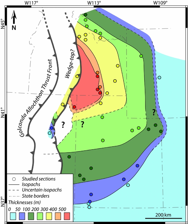
Figure 8. Isopach map of the sedimentary thicknesses recorded for the PTU-Smithian interval, showing marked differences in sedimentary thicknesses between northern and southern Sonoma Foreland Basin. The studied sections are shown at their palaeolocation (Fig. 7). The reconstructed Golconda Allochthon Thrust Front during the PTU-Smithian studied interval is also indicated (modified from Dickinson, Reference Dickinson2013; see also Fig. 12). The position of the wedge-top is based on variations in the sedimentary thicknesses and on geophysical data (Fig. 10).
The subsidence analysis (Fig. 9) also shows a clear distinction between the northern and southern parts of the basin. Confusion Range (CR, Fig. 9a) and Pahvant Range (PR, Fig. 9b) sections exhibit relatively low subsidence curves during the studied interval, whereas Sheep Creek (SC, Fig. 9c) and Hot Springs (HS, Fig. 9d) sections show a high subsidence profile. The total and tectonic subsidence curves are similar and the tectonic subsidence is here a major component of the total subsidence, accounting for at least two-thirds of the total subsidence, if not more (e.g. in CR, Fig. 9a).
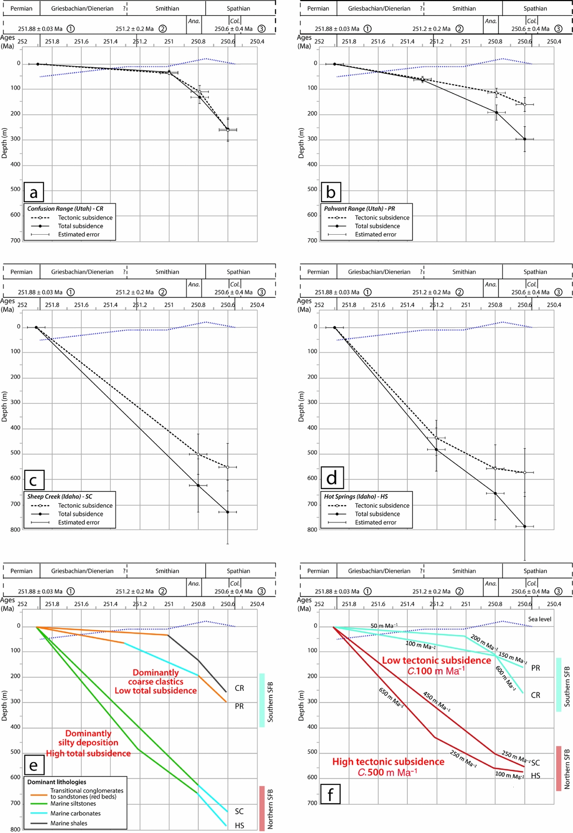
Figure 9. Subsidence analysis results obtained for the PTU-Smithian interval and early Spathian time using 1D backstripping (Steckler & Watts, Reference Steckler and Watts1978; Van Hinte, Reference Van Hinte1978; Allen & Allen, Reference Allen and Allen2005). Locations of sections are given in Figure 3b. Ages for the bottom and top boundaries of the Smithian are interpolated from ammonoid biozone durations (after Brühwiler et al. Reference Brühwiler, Bucher, Brayard and Goudemand2010). Sea-level curve after Haq, Hardenbol & Vail (Reference Haq, Hardenbol, Vail, Wilgus, Hastings, Posamentier, Wagoner, Ross and Kendall1988). Ana.: Anasibirites beds; Col.: Columbites beds. Radiometric ages from (1) Burgess, Bowring & Shen (Reference Burgess, Bowring and Shen2014); (2) and (3) Galfetti et al. (Reference Galfetti, Bucher, Ovtcharova, Schaltegger, Brayard, Brühwiler, Goudemand, Weissert, Hochuli, Cordey and Guodun2007). Subsidence analysis for: (a) Confusion Range (CR) section; (b) Pahvant Range (PR) section; (c) Sheep Creek (SC) section; (d) Hot Springs (HS) section. (e) Total subsidence curves for all the CR, PR, SC and HS sections and associated dominant lithologies are indicated for each subinterval. (f) Tectonic subsidence curves for the CR, PR, SC and HS sections and associated mean tectonic subsidence rates. (e) and (f) allow two distinct subsidence dynamics to be discriminated between the southern and northern parts of the SFB.
When looking at the dominant lithologies (Fig. 9e), the sections from the southern part of the basin display a sedimentary succession dominated by coarse conglomerates and sandstones and microbial limestones of the Moenkopi Group and the limestones/shales of the Thaynes Group (Figs 3, 4, 9e), while the total subsidence is low. By contrast, the sections from the northern part of the SFB are dominated by fine siltstones (Figs 3, 4, 9e) with an important subsidence.
Finally, the tectonic subsidence appears as a critical diagnostic feature for the basin (Fig. 9f). A marked difference exists between mean tectonic subsidence rates in the southern and northern parts of the basin (c. 100 m Ma–1 v. c. 500 m Ma–1, respectively). The southern sections show a low-rate tectonic subsidence (50–200 m Ma–1; Fig. 9e). Nevertheless, a marked increase in subsidence rate is recorded during early Spathian time for these sections (150–600 m Ma–1; Fig. 9e). Conversely, the northern sections show a higher rate of tectonic subsidence during the PTU-Smithian interval (450–650 m Ma–1; Fig. 9e), whereas early Spathian time is characterized by a decrease in subsidence rate (100–250 m Ma–1; Fig. 9e).
4.b. Basement characterization
On the gravimetric anomaly map shown on Figure 10a, black lines outline the geophysical features that may represent traces of crustal/lithospheric faults or heterogeneities in the basement (Lowrie, Reference Lowrie2007). The lowest Bouguer anomaly values (<150 mGal, Fig. 10a) suggest the presence of a thick crust, whereas moderate negative anomalies (between –65 and –135 mGal; white outlines) point towards a thinner crust and/or the presence of lower-crustal high-density bodies (e.g. Gilbert, Velasco & Zandt, Reference Gilbert, Velasco and Zandt2007; Lowrie, Reference Lowrie2007). The Snake River Plain (SRP in Fig. 10a) is a Yellowstone hotspot track-related basaltic province. This young (of Neogene age) structure influences neither the geometry nor the properties of the basement (Dickinson, Reference Dickinson2013). The Farmington Anomaly (FA on Fig. 10a), located in the centre of the study area, may result from the presence of lower-crustal high-density mafic and/or ultramafic material emplaced during a thermal event dated at c. 1.64 Ga (Mueller et al. Reference Mueller, Wooden, Mogk and Foster2011). Alternatively, it can have originated from a more recent thermal event and/or the presence of a thin lithospheric crust (e.g. Gilbert, Velasco & Zandt, Reference Gilbert, Velasco and Zandt2007; Lowrie, Reference Lowrie2007). Remnants of an important thermal metamorphism including partial melting (c. 1.67 Ga) can also be observed in this area (red dots in Fig. 10c; Mueller et al. Reference Mueller, Wooden, Mogk and Foster2011). The Southern Anomaly (SA on Fig. 10a) is poorly documented and may result from variations in the crustal thickness of the terrane (e.g. Gilbert, Velasco & Zandt, Reference Gilbert, Velasco and Zandt2007; Lowrie, Reference Lowrie2007), possibly linked to the Ancestral Rocky Mountains orogeny or to the more recent Laramide orogeny and the building of the Rocky Mountains (Ye et al. Reference Ye, Royden, Burchfiel and Schuepbach1996; Dickerson, Reference Dickerson2003).
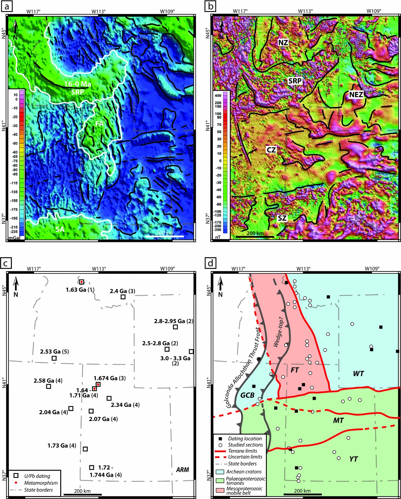
Figure 10. (a) Bouguer gravity anomaly map of the Sonoma Foreland Basin and its surroundings (in mGal; after Kucks, Reference Kucks1999). Notable moderate gravity anomalies are highlighted by a white contour. SRP: Snake River Plain; FA: Farmington Anomaly; SA: Southern Anomaly. Black lines represent the interpreted remnants of the main geophysical accidents, and limits between crustal features. (b) Aeromagnetic anomaly map of the Sonoma Foreland Basin and its surroundings (in nT; after Bankey et al. Reference Bankey, Cuevas, Daniels, Finn, Hernandez, Hill, Kucks, Miles, Pilkington, Roberts, Roest, Rystrom, Shearer, Snyder, Sweeney, Velez, Phillips and Ravat2002). Black lines highlight areas of contrasted magnetic signatures: SRP: Snake River Plain; SZ: Southern magnetic Zone; CZ: Central magnetic Zone; NEZ: North-Eastern magnetic Zone; NZ: Northern magnetic Zone. (c) Map of the spatial location of the radiochronological ages (U/Pb ages) after: (1) Foster et al. Reference Foster, Mueller, Mogk, Wooden and Vogl2006; (2) Fan et al. Reference Fan, DeCelles, Gehrels, Dettman, Quade and Peyton2011; (3) Mueller et al. Reference Mueller, Wooden, Mogk and Foster2011; (4) Nelson, Hart & Frost, Reference Nelson, Hart and Frost2011; (5) Strickland, Miller & Wooden, Reference Strickland, Miller and Wooden2011). Superimposed red dots indicate Mesoproterozoic metamorphism episodes (Mueller et al. Reference Mueller, Wooden, Mogk and Foster2011). (d) Map of basement terranes of the SFB according to their age and nature, with Archean terranes (pale blue), Palaeoproterozoic terranes (pale green) and Mesoproterozoic mobile belt (pale red). FT: Farmington Terrane; GCB: Grouse Creek Block; MT: Mojave Terrane; WT: Wyoming Terrane; YT: Yavapai Terrane.
The aeromagnetic anomaly map presented in Figure 10b discriminates areas of contrasted magnetic signatures (separated by black lines on Fig. 10b). These disturbances in magnetic field are attributed to differences in the nature of the rocks composing the basement (Turner, Rasson & Reeves, Reference Turner, Rasson and Reeves2007). We do not attempt to identify the exact nature of these rocks here; rather, we use these contrasted anomalies to characterize differences of rock types that compose the basement (Purucker & Whaler, Reference Purucker and Whaler2007; Lund et al. Reference Lund, Box, Holm-Denoma, San Juan, Blakely, Saltus, Anderson and Dewitt2015). As on the Bouguer gravity anomaly map, the presence of the Snake River Plane hotspot-track (SRP in Fig. 10a, b) is obvious on the aeromagnetic anomaly map. It features a strong positive magnetic anomaly signal (>150 nT, Fig. 10b). The Southern magnetic Zone (SZ on Fig. 10b) can be distinguished on the southern part of the studied area by contrasted anomalies with a wide range of variations (from c. –200 nT up to c. 400 nT). The Central magnetic Zone (CZ on Fig. 10b) occupies the central third of the map. It is characterized by generally neutral to (strongly) positive anomalies (from c. –10 nT to c. 60 nT, locally up to >150 nT). In the northeastern quarter of the studied area, the North-Eastern magnetic Zone (NEZ on Fig. 10b) is characterized by generally negative anomalies (between c. –80 nT and c. –10 nT). Some areas with strong positive anomalies (>150 nT) are also observed, whose shape and extension are very similar in the Bouguer gravity anomaly map (Fig. 10a). Finally, a small Northern magnetic Zone (NZ on Fig. 10b) is visible north to the SRP and west to the NZ. It shows contrasting anomalies, but with a less important range of variation than the SRP and less strongly positive values (from c. –60 nT to c. 150 nT only).
Figure 10c synthesizes the location and the different U/Pb radiochronological ages for the basement (Foster et al. Reference Foster, Mueller, Mogk, Wooden and Vogl2006; Fan et al. Reference Fan, DeCelles, Gehrels, Dettman, Quade and Peyton2011; Mueller et al. Reference Mueller, Wooden, Mogk and Foster2011; Nelson, Hart & Frost, Reference Nelson, Hart and Frost2011; Strickland, Miller & Wooden, Reference Strickland, Miller and Wooden2011). Basement rocks of Archean, Palaeoproterozoic and Mesoproterozoic ages can be found throughout the entire studied area (Fig. 10c). Archean ages are found in Wyoming, southwestern Montana and northeastern Nevada (Fig. 10c; Fan et al. Reference Fan, DeCelles, Gehrels, Dettman, Quade and Peyton2011; Mueller et al. Reference Mueller, Wooden, Mogk and Foster2011; Nelson, Hart & Frost, Reference Nelson, Hart and Frost2011; Strickland, Miller & Wooden, Reference Strickland, Miller and Wooden2011). Palaeoproterozoic ages are found in Utah and eastern Nevada (Fig. 10c; Mueller et al. Reference Mueller, Wooden, Mogk and Foster2011; Nelson, Hart & Frost, Reference Nelson, Hart and Frost2011). Finally, Mesoproterozoic ages associated with metamorphism are found in northwestern Utah and northern Idaho (Fig. 10c; Foster et al. Reference Foster, Mueller, Mogk, Wooden and Vogl2006; Mueller et al. Reference Mueller, Wooden, Mogk and Foster2011; Nelson, Hart & Frost, Reference Nelson, Hart and Frost2011).
Five different lithospheric terranes composing the SFB basement can therefore be identified: the Wyoming Terrane (WT); the Grouse Creek Block (GCB); the Mojave Terrane (MT); the Yavapai Terrane (YT); and the Farmington Terrane (FT; Fig. 10d). The GCB and WT are Archean terranes with ages of c. 2.5 Ga (Nelson, Hart & Frost, Reference Nelson, Hart and Frost2011; Strickland, Miller & Wooden, Reference Strickland, Miller and Wooden2011) and 2.4–3.3 Ga (Fan et al. Reference Fan, DeCelles, Gehrels, Dettman, Quade and Peyton2011; Mueller et al. Reference Mueller, Wooden, Mogk and Foster2011), respectively. The MT is a Palaeoproterozoic terrane of age 2.04–2.34 Ga, whereas the YT is a younger Palaeoproterozoic terrane of age 1.720–1.744 Ga (Nelson, Hart & Frost, Reference Nelson, Hart and Frost2011). The FT is a Mesoproterozoic intracratonic mobile belt (Lund et al. Reference Lund, Box, Holm-Denoma, San Juan, Blakely, Saltus, Anderson and Dewitt2015) composed of reworked Archean crust (Whitmeyer & Karlstrom, Reference Whitmeyer and Karlstrom2007), with metamorphism ages between 1.63 and 1.71 Ga (Foster et al. Reference Foster, Mueller, Mogk, Wooden and Vogl2006; Mueller et al. Reference Mueller, Wooden, Mogk and Foster2011; Nelson, Hart & Frost, Reference Nelson, Hart and Frost2011).
4.c. Impact of the heritage on the SFB development
The fact that the basement of the SFB is composed of five Archean–Mesoproterozoic terranes questions the potentially crucial role of inherited lithospheric features on the formation and spatio-temporal evolution of the SFB.
Lithospheric strength (i.e. rigidity) of the terranes varies depending on their age and heritage (Poudjom Djomani et al. Reference Poudjom Djomani, O'Reilly, Griffin and Morgan2001; Artemieva & Mooney, Reference Artemieva and Mooney2002), with important changes in rheological behaviour and segregation between oldest (>1.7 Ga) and juvenile crusts (<1.7 Ga; Artemieva & Mooney, Reference Artemieva and Mooney2002). Since older lithospheres are more rigid than younger, Archean and Palaeoproterozoic basements such as the Wyoming Terrane, Grouse Creek Block, Mojave Terrane and Yavapai Terrane are defined here as ‘strong’ lithospheres (e.g. Cardozo & Jordan, Reference Cardozo and Jordan2001; Leever et al. Reference Leever, Matenco, Bertotti, Cloetingh and Drijkoningen2006; Fig. 11). Conversely, the more recent Mesoproterozoic lithospheres such as the Farmington Terrane (Fig. 11) are characterized by a lower rigidity (e.g. Cardozo & Jordan, Reference Cardozo and Jordan2001; Leever et al. Reference Leever, Matenco, Bertotti, Cloetingh and Drijkoningen2006; Fosdick, Graham & Hilley, Reference Fosdick, Graham and Hilley2014). Additionally, some lithospheres can be weaker than coeval ones due to their structural heritage and thermal history, and are assumed to be ‘attenuated’ (sensu Fosdick, Graham & Hilley, Reference Fosdick, Graham and Hilley2014). The Farmington Terrane was formed as a mobile belt between Archean GCB and WT and underwent at least one event of intense thermal metamorphism during Mesoproterozoic time (Mueller et al. Reference Mueller, Wooden, Mogk and Foster2011; Lund et al. Reference Lund, Box, Holm-Denoma, San Juan, Blakely, Saltus, Anderson and Dewitt2015) Younger occurrences of similar events until Early Triassic time cannot be ruled out, especially given the Bouguer gravity anomaly hints of underplating dense material (see Section 4.b). The Farmington Terrane is therefore considered here as a ‘thermally attenuated weak’ lithosphere (Fig. 11).
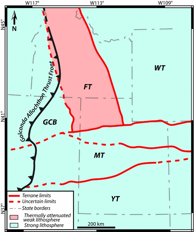
Figure 11. Map of the SFB basement (cf. Fig. 10d) after their heritage and therefore their rheological behaviour. Archean Grouse Creek Block and Wyoming Terrane, Palaeoproterozoic Mojave Terrane and Yavapai Terrane are considered ‘strong’ lithospheres with an important rigidity (pale blue), while the Mesoproterozoic mobile belt Farmington Terrane is considered a ‘thermally attenuated weak’ lithosphere due to its lesser rigidity (pale red).
Due to the lithospheric heterogeneity of the basement, the role of the boundary lithospheric faults can be considered as essential. Neoarchean–Palaeoproterozoic terranes are limited by mega-shear zones along with deep (nearly) vertical crustal and/or lithospheric faults (Figs 10d, 11). Terranes in the SFB display some characteristics (e.g. dimension, geometry) that are similar to the terranes associated with the Neoarchean–Palaeoproterozoic accretionary orogens (e.g. Chardon, Gapais & Cagnard, Reference Chardon, Gapais and Cagnard2009; Cagnard, Barbey & Gapais, Reference Cagnard, Barbey and Gapais2011). These lithospheric and crustal accidents have therefore been reactivated since their Precambrian onset (e.g. Bryant & Nichols, Reference Bryant and Nichols1988; Paulsen & Marshak, Reference Paulsen and Marshak1999). Additionally, several authors (e.g. Eardley, Reference Eardley1939; Peterson, Reference Peterson and Helsey1977) identified the presence of a topographic basement highland (pale blue area in Fig. 12a, in colour online) near the junction between the MT and the GCB/FT/WT during Palaeozoic time, separating the northern and southern areas of marked sedimentary accumulation. Eardley (Reference Eardley1939) first introduced this feature as the ‘Northern Utah Highland’. Peterson (Reference Peterson and Helsey1977) highlighted its presence on his palinspastic maps for the Palaeozoic stratigraphic record. Finally, this sedimentary and topographic pattern seems to have been the same in this basin since Proterozoic time (Paulsen & Marshak, Reference Paulsen and Marshak1999; Fig. 12a).
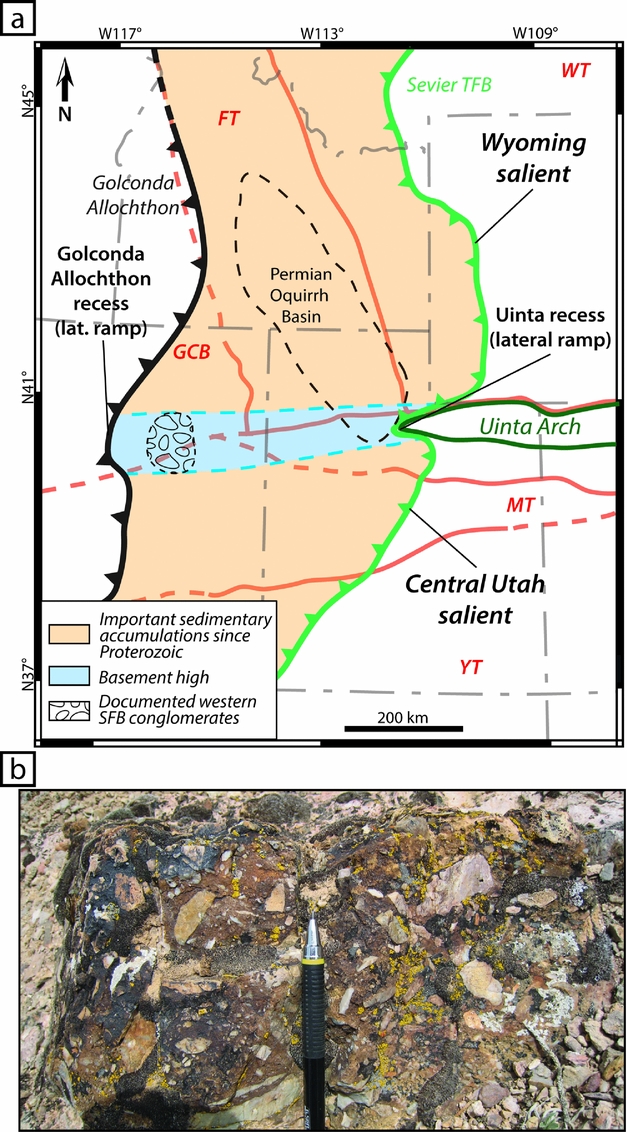
Figure 12. (a) Simplified map showing the position of the Uinta recess (lateral ramp) and Wyoming and Central Utah salients (frontal ramps) of the present-day Sevier TFB (after Paulsen & Marshak, Reference Paulsen and Marshak1999; Yonkee & Weil, Reference Yonkee and Weil2010) and reconstructed Golconda Allochthon front and associated recess (lateral ramp). Sedimentary pattern since Proterozoic time shows two high accommodation zones separated by a topographic high close to the terrane boundaries (Peterson, Reference Peterson and Helsey1977, Bryant & Nichols, Reference Bryant and Nichols1988; Paulsen & Marshak, Reference Paulsen and Marshak1999). Palaeolocation of Permian Oquirrh Basin (e.g. Yonkee & Weil, Reference Yonkee and Weil2015) and documented PTU-Smithian conglomerates in the western SFB (e.g. Gabrielse, Snyder & Stewart, Reference Gabrielse, Snyder and Stewart1983; Lucas & Orchard, Reference Lucas and Orchard2007) are also included on the map. Red lines indicate limits of the basement terranes (cf. Fig 9d). (b) Photograph (courtesy of Hugo Bucher, Zürich) of the conglomerates found in the area delimited in (a), presumably a product of western relief dismantlement.
By the time of the initiation of the Sonoma orogeny, this difference in sedimentary accumulation was well marked in Palaeozoic series (Peterson, Reference Peterson and Helsey1977). For instance, about 6 km of marine sediments accumulated in the Permian Oquirrh Basin in the northern part of the SFB (Fig. 12a; Yonkee & Weil, Reference Yonkee and Weil2015), whereas the southern part of the SFB saw the deposition of only several hundred metres of marine and terrigenous sediments (e.g. c. 640 m in southwestern Utah; Rowley et al. Reference Rowley, Vice, Mcdonald, Anderson, Machette, Maxwell, Ekrem, Cunningham, Steven and Wardlaw2005) during the same interval. The thick Palaeozoic sedimentary series in northern and southern parts of the foreland (Peterson, Reference Peterson and Helsey1977) would have allowed the thrust belt to propagate, while the presence of the topographic basement highland characterized by a reduced sedimentary cover should have triggered the formation of a lateral ramp and a recess in the central part of the front (Fig. 12a). The presence of the topographic high is attested by the occurrence of shallow conglomerates in the western part of the SFB within the PTU-Smithian interval (Fig. 12a, b; e.g. Gabrielse, Snyder & Stewart, Reference Gabrielse, Snyder and Stewart1983; Lucas & Orchard, Reference Lucas and Orchard2007; Jattiot et al., in press). Previous reconstruction of the GA thrust front also accounted for the presence of a recess in the central part of the thrust front (e.g. Dickinson, Reference Dickinson2006, Reference Dickinson2013). Moreover, this mechanism underlying the observed differential propagation has been proposed by Paulsen & Marshak (Reference Paulsen and Marshak1999) for the Sevier thrust-and-fold belt which shows the presence of a lateral ramp in its central part (Fig. 2). This was explained by the pre-deformational sedimentary thicknesses pattern showing thrusts propagating further when emplaced upon a thicker sedimentary cover (Figs 2, 12a; Paulsen & Marshak, Reference Paulsen and Marshak1999). It is worth noting that both the lateral ramps of the Sevier and Golconda thrust-and-fold belt are located close to and along the lithospheric boundary between the MT and FT/WT (Figs 2, 12a).
The GA heterogeneity may therefore have played a role, complementary to the basement heritage, over the flexural response of the SFB. However, due to the scarcity of allochthon remnants, a numerical model is required to decipher its potential role.
4.d. Simulating the flexural response of the basin
All the data discussed above have been integrated in a 2D numerical flexural model. This approach allows us to quantify in a predictive way the flexural behaviour of the basin in relation to its basement heritage.
4.d.1. Numerical approach and setup
The 2D plane stress flexural models have been solved with a finite element method code written in Matlab® (Le Pourhiet & Saleeby, Reference Le Pourhiet and Saleeby2013; Moreau et al. Reference Moreau, Le Pourhiet, Huuse, Gibbard and Grappe2015). It solves
 $$\begin{equation}
{{\nabla ^{\rm{2}}}\left( {D{\nabla ^{\rm{2}}}\omega } \right) = g\left( {{\rho _{\rm{m}}} - {\rho _{\rm{i}}}} \right) + q}
\end{equation}$$
$$\begin{equation}
{{\nabla ^{\rm{2}}}\left( {D{\nabla ^{\rm{2}}}\omega } \right) = g\left( {{\rho _{\rm{m}}} - {\rho _{\rm{i}}}} \right) + q}
\end{equation}$$
for flexural deflection ω of a thick elastic plate (Reissner–Mindlin approximation) using bilinear isoparametric elements with under integration technique for the shear terms (Zienkiewicz & Taylor, Reference Zienkiewicz and Taylor2005). In Equation (1) the rigidity of the plate D, defined
 $$\begin{equation*}
{D = \frac{{E{T_{\rm{e}}}^3}}{{12\left( {1 - {\nu ^2}} \right)}}},
\end{equation*}$$
$$\begin{equation*}
{D = \frac{{E{T_{\rm{e}}}^3}}{{12\left( {1 - {\nu ^2}} \right)}}},
\end{equation*}$$
depends solely on the effective elastic thickness T e as the plate Young's modulus E and Poisson's ratio ν are fixed at 80 GPa and 0.25, respectively (Burov & Diament, Reference Burov and Diament1995). The topographic loads q = ρ t g h account for the thickening h resulting from the orogeny and are computed using a density ρ t = 2700 kg m–3. The mantle restoring forces are computed assuming a density ρ m = 3300 kg m–3, while the infill is considered to be sediments of density ρ i =1600 kg m–3. We arbitrarily attributed a constant height h = 1500 m to the topographic load as we concentrate on the effect of heterogeneities of the allochthon morphology and rheology of the basement only. These initial parameters are summarized in Table 2.
Table 2. Summary of model parameters for the SFB and tested scenarii.
The models are 907 km wide in the x direction, chosen to be normal to the trend of the orogenic belt, and 1166 km in the y direction. We assume that isostatic compensation is achieved underneath the orogen and, accordingly, we set the curvature normal to the right side to zero, ∂ω/∂x = 0. As the orogen is very long compared to the region where flexural subsidence is analysed, we enforce cylindrical boundary conditions on the side of normal y (∂ω/∂y = 0). On the right boundary, that is, far from the orogeny, the effect of topographic loading can be considered null, corresponding to ω = 0.
In this model, we used T e1 = 90 km for the ‘strong’ GCB, WT, MT and YT lithospheres (Table 2), which is a good approximation for cratonic T e (Watts, Reference Watts1992). The ‘weak-attenuated’ FT is expected to show a contrasted lower T e value due to its assumed rheological weaknesses. This value was set at T e2 = 30 km (Table 2; e.g. Leever et al. Reference Leever, Matenco, Bertotti, Cloetingh and Drijkoningen2006).
4.d.2. Model results
Figure 13 shows that the southern part of the front is reconstructed as less propagated into the foreland than the northern part (Fig. 12a; see Dickinson, Reference Dickinson2006, Reference Dickinson2013). In this model, the lateral ramp is spatially restricted along the limit between the FT/WT and MT (Fig. 13a). The northern part, emplaced mainly above the ‘weak’ FT and in front of the largest part of the GA, presents a narrower foredeep with λ ≈ 250 km (Fig. 13a, b). The steep foredeep is bordered by a well-expressed forebulge emplaced close to the FT/WT boundary (Fig. 13a; XX’ in Fig. 13b). The southern part of the foreland is set upon ‘strong’ lithospheres (MT and YT) in front of the smallest and recessed parts of the GA (Fig. 13a, c). The foredeep in this part of the model is larger, with λ ≈ 320 km, and its profile (YY’ in Fig. 13c) also exhibits a weaker topography than in the northern part. We also notice the presence of a barely expressed forebulge in this area (Fig. 13a, c).
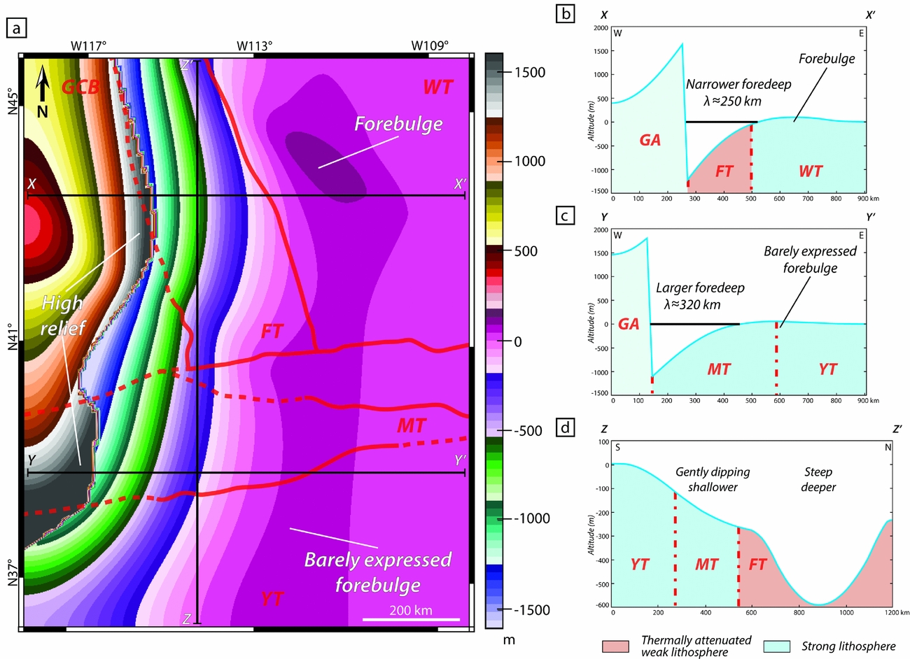
Figure 13. Numerical model of the SFB after the reconstructed palaeogeography and terranes map (cf. Figs 11, 12) with an heterogeneous basement (‘strong’ v. ‘thermally attenuated weak’ lithospheres) and an heterogeneous allochthon (recessed area in central part of the front). (a) Simulated map of the SFB. Thin black lines indicate the position of the 2D profiles; red lines indicate limits of the basement terranes (cf. Fig 10d). (b) 2D W–E profile of the northern part of the SFB model. The narrow foredeep is emplaced upon the ‘thermally attenuated weak’ FT and is bordered by a well expressed forebulge. (c) 2D W–E profile of the southern part of the SFB model. The wider foredeep is emplaced upon the ‘strong’ MT, and is bordered by a barely expressed forebulge. (d) 2D S–N profile of the SFB model. The two northern and southern parts of the basin are individualized with a limit near the MT/FT boundary.
The dichotomy between the northern and southern parts is especially obvious on a S–N transect (ZZ’ in Fig. 13d). A shallow southern sub-basin with a gentle northwards dip (< c. 250 m deep) is identified, as well as a northern deeper basin with steep borders (c. 600 m deep). The limit between the northern and southern parts appears relatively close to the MT/FT boundary (Fig. 13d), suggesting a significant role for lithospheric boundaries in the differential flexuration of the SFB. This N–S differentiation is found not only in the foreland, but also within the allochthon itself as its simulated elevation is not continuous along its front (Fig. 13a). Two areas of important elevations (>1200 m) can be observed on both the northern and southern sides of the GA recess. This positive relief could have contributed as a significant source of terrigenous material, then being deposited in the proximal foreland.
5. Discussion
Our results highlight the spatial differences in subsidence within the SFB, especially between its northern and southern parts (Figs 8, 9). This differential subsidence is underlined by variations in the sedimentary record (Figs 4, 5). In addition, a highland was probably present in the central SFB and could physically have partly separated these two parts of the basin.
5.a. Evidence for a foreland basin
The convex ‘lozenge shape’ (sensu Miall, Reference Miall2010) of the isopach map (Fig. 8) and the westwards-thickening pattern of the sedimentary record are in agreement with the common asymmetric geometry of foreland basins (Fig. 8; DeCelles & Giles, Reference DeCelles and Giles1996; Miall, Reference Miall2010). Additionally, the observed high-rate subsidence values (c. 100–500 m Ma–1) agree with foreland basin dynamics, even if these values are greater in magnitude than values generally given in the literature for similar contexts (e.g. Xie & Heller, Reference Xie and Heller2009). This difference in magnitude is interpreted by considering that estimations from backstripping analyses are generally proposed for continuous sedimentary series spanning several millions years, if not several tenth of millions years (e.g. Xie & Heller, Reference Xie and Heller2009). Over such long time intervals, the subsidence rate values are less accurate. The high resolution of the timeframe used for the SFB mirrors short-acting structural events in the basin. Similar ‘higher than average’ values for subsidence rates have been calculated by Chevalier et al. (Reference Chevalier, Guiraud, Garcia, Dommergues, Quesne, Allemand and Dumont2003) and Lachkar et al. (Reference Lachkar, Guiraud, El Harfi, Dommergues, Dera and Durlet2009) using high-resolution biostratigraphic time-calibrations, and also by Roddaz et al. (Reference Roddaz, Hermoza, Mora, Baby, Parra, Christophoul, Brusset, Espurt, Hoorn and Wesselingh2010) with similar magnitude for the Miocene Amazonian Foreland Basin (c. 200–700 m Ma–1; Roddaz et al. Reference Roddaz, Hermoza, Mora, Baby, Parra, Christophoul, Brusset, Espurt, Hoorn and Wesselingh2010). Moreover, values observed in the SFB (0.05–0.65 mm a–1) are consistent with yearly deposition rates indicated by Allen & Allen (Reference Allen and Allen2005) for foreland basins (0.2–0.5 mm a–1). Finally, the convex-up shape of the tectonic subsidence curves (Fig. 9f) is diagnostic of foreland basins and corresponds to the progressive flexural response of the lithosphere to the topographic load and/or sedimentary infill of the basin overtime (Angevine, Heller & Paola, Reference Angevine, Heller and Paola1990; Allen & Allen, Reference Allen and Allen2005; Xie & Heller, Reference Xie and Heller2009).
In the SFB, the topographic load is exerted by the GA. This allochthon has been emplaced on the North American continental margin, as evidenced by the geochemical signature of the Koipato Formation volcanics (Early Triassic) originating from the partial melting of a Palaeoproterozoic continental crust (likely the Mojave Terrane; Vetz, Reference Vetz2011).
The observed spatial heterogeneity of the sedimentary thickness in the SFB (Figs 4, 8) and the much higher tectonic subsidence rate detected in the northern part of the basin (c. 500 m Ma–1 v. c. 100 m Ma–1 in the southern part; Fig. 9f) are striking and raise the question of the controlling factor(s) responsible for this phenomenon, especially for such a short interval (c. 1.3 Ma).
5.b. Potential underlying mechanisms for observed variations in flexural subsidence
Spatial variations in subsidence within the SFB may result from different mechanisms that are inherent to the flexural nature of the foreland basin: (1) the sedimentary overload provoked by the continuous filling of the basin over time; (2) the spatial heterogeneity of the GA (topography and shape of the load); and/or (3) the differential flexural response of the lithosphere to this topographic load and linked to the rheology of the basement.
Considering point (1) above, in some cases the distributed vertical load exerted by the sedimentary filling of the basin might affect and amplify the flexuration in foreland basins over time (Shanmugam & Walker, Reference Shanmugam and Walker1980; Beaumont, Reference Beaumont1981; Cardozo & Jordan, Reference Cardozo and Jordan2001; Allen & Allen, Reference Allen and Allen2005). As this load depends mainly on the sedimentary fluxes and density of the filling, a denser deposited material leads to a more important flexuration of the lithosphere, as modelled by Angevine, Heller & Paola (Reference Angevine, Heller and Paola1990) and Fosdick, Graham & Hilley (Reference Fosdick, Graham and Hilley2014). The southern part of the SFB, characterized by low subsidence rates, exhibits coarse clastic sedimentation in the Moenkopi Group with the presence of conglomerates and sandstones (Figs 3a, 4, 5b, c, e, 12; e.g. Gabrielse, Snyder & Stewart, Reference Gabrielse, Snyder and Stewart1983; Olivier et al. Reference Olivier, Brayard, Vennin, Escarguel, Fara, Bylund, Jenks, Caravaca and Stephen2016) of density 2.5–2.8 kg cm−3 (Manger, Reference Manger1963; McCulloh, Reference McCulloh1967; Sclater & Christie, Reference Sclater and Christie1980; Tenzer et al. Reference Tenzer, Sirguey, Rattenbury and Nicolson2011). The top of the Moenkopi Group consists of thick microbial limestone beds (Figs 3a, 4, 5e; e.g. Olivier et al. Reference Olivier, Brayard, Fara, Bylund, Jenks, Vennin, Stephen and Escarguel2014, Reference Olivier, Brayard, Vennin, Escarguel, Fara, Bylund, Jenks, Caravaca and Stephen2016; Vennin et al. Reference Vennin, Olivier, Brayard, Bour, Thomazo, Escarguel, Fara, Bylund, Jenks, Stephen and Hofmann2015). These limestones bear a density of c. 2.6–2.8 kg cm−3 (Manger, Reference Manger1963; McCulloh, Reference McCulloh1967; Sclater & Christie, Reference Sclater and Christie1980; Tenzer et al. Reference Tenzer, Sirguey, Rattenbury and Nicolson2011). In contrast, the northern part which is characterized by high subsidence rates, is dominated by marine siltstones of the Dinwoody and Woodside Formation (Figs 3a, 4, 5g; e.g. Kummel, Reference Kummel1954, Reference Kummel and Ladd1957). The density of this type of sediment is of 2.3–2.7 kg cm−3 (Manger, Reference Manger1963; Sclater & Christie, Reference Sclater and Christie1980; Tenzer et al. Reference Tenzer, Sirguey, Rattenbury and Nicolson2011). Based on these data, the sedimentary filling should have had a higher impact on the flexuration in the southern part of the basin. However, we show that the most important subsidence during the PTU-Smithian interval took place in the northern part of the SFB (Figs 8, 9). Moreover, the difference between tectonic and total subsidence mainly consist of the local isostasy and compaction of the sediments (Allen & Allen, Reference Allen and Allen2005). With the tectonic subsidence being the most important component of the total subsidence in the SFB (Fig. 9a), this argues for a weak potential role of the sedimentary load. The sedimentary overload therefore cannot be a major controlling factor explaining the differential flexuration observed within the basin.
Regarding points (2) and (3) above, while it is possible to discuss the role of the sedimentary overload using only field-based data, interpretations of the allochthon heterogeneity and the basement rheological behaviour require an additional model approach. We combine these in the following discussion. To that purpose, we used three different scenarios (Fig. 14) with the same initial setup (Section 4.d; Table 2) except for the x and y dimensions of the model that are set to 2000 km in the x direction and 1000 km in the y direction to avoid border effects.
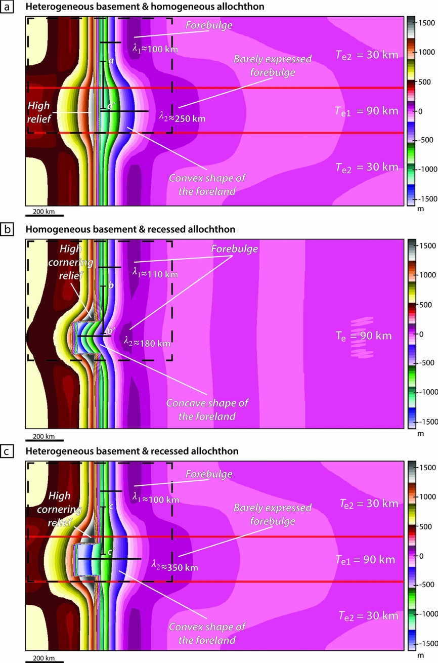
Figure 14. Numerical models showing the effects of the heterogeneities of the basement and of the topographic load over the formation of a foreland basin. Dashed lines represent an area analogue to the SFB configuration. (a) Scenario using a heterogeneous basement with contrasted elastic thicknesses (T e1 = 3×T e2) and a homogeneous allochthon. A large convex foreland is formed upon the most rigid lithosphere. (b) Scenario using a heterogenous allochthon with a c. 100 km wide recess (lateral ramp) and a homogeneous fixed T e lithosphere. A slightly wider concave foreland is formed within the recessed area and a cornering relief appears on both sides of the recessed area in the allochthon. (c) Scenario showing the combined effect of a heterogeneous basement with contrasted elastic thicknesses (T e1 = 3×T e2) and a heterogeneous allochthon with a c. 100 km wide recess (lateral ramp). A much wider convex foreland is formed within the recessed area upon the rigid lithosphere, and a cornering relief on both sides of the recess in the allochthon is also visible.
The first scenario tests the impact of a rheologically heterogeneous basement loaded by a homogeneous allochthon (Fig. 14a). The rigidity of the terrane controls its capacity to flexure. The shape of ensuing flexural foreland basins and the distribution of their sedimentary records are therefore a direct consequence of the rheological behaviour of the basement (Angevine, Heller & Paola, Reference Angevine, Heller and Paola1990; Watts, Reference Watts1992; Cardozo & Jordan, Reference Cardozo and Jordan2001; Allen & Allen, Reference Allen and Allen2005; Leever et al. Reference Leever, Matenco, Bertotti, Cloetingh and Drijkoningen2006; Fosdick, Graham & Hilley, Reference Fosdick, Graham and Hilley2014). Upon the high-rigidity part of the basement (T e1), a wide foreland (λ 2 ≈ 250 km) develops with a well-expressed convex shape in map view and a barely expressed forebulge. Upon the low-rigidity parts of the basement (T e2), a narrower foreland (λ 1 ≈ 100 km) is structured with a more pronounced forebulge. This is in agreement with the SFB observations. However, a N–S transect (aa’, Fig. 14a) shows that the wider area of the foreland basin is deeper than observed in the field and that only one high-relief area is individualized within the central part of the allochthon. Even if the rigidity does play a role in the development of the flexural foreland basin, as commonly assumed in the literature (Angevine, Heller & Paola, Reference Angevine, Heller and Paola1990; DeCelles & Giles, Reference DeCelles and Giles1996; Cardozo & Jordan, Reference Cardozo and Jordan2001; Allen & Allen, Reference Allen and Allen2005; Leever et al. Reference Leever, Matenco, Bertotti, Cloetingh and Drijkoningen2006; Miall, Reference Miall2010; Fosdick, Graham & Hilley, Reference Fosdick, Graham and Hilley2014), our results indicate that a rheological difference is not enough to control the variations in SFB.
The second scenario uses a heterogeneous topographic load exerted by the allochthon upon a homogeneous ‘strong’ lithosphere (T e = 90 km; Fig. 14b). The heterogeneity in the allochthon is introduced in the form of a c. 100 km wide recess (i.e. a lateral ramp) along its front. The foreland basin shows a larger area (λ 2 ≈ 180 km) in front of the lateral ramp compared to the northern and southern parts (λ 1 ≈ 110 km). Moreover, a N–S transect (bb’ in Fig. 14b) shows that the narrow northern part of the basin is deeper than in front of the recess. An important relief is also formed in the corners of the allochthon on both lateral borders of the recess. This is in agreement with SFB observations. However, the overall shape of the foreland basin is rather concave and penetrates significantly into the recessed area. Even if the morphology of the allochthon plays a role in the development of the foreland basin, this numerical scenario shows marked differences with the SFB.
The third scenario combines both previously tested heterogeneities (Fig. 14c). The graphic output exhibits a wider foreland (λ 2 ≈ 350 km) emplaced above the ‘strong’ lithosphere in front of the recess, and a narrow foreland (λ 1 ≈ 100 km) above ‘weak’ lithospheres. This model reproduces well the convex shape of the foreland basin with a marked forebulge development upon ‘weak’ lithospheres, whereas it is less pronounced upon the strong lithosphere. Moreover, a N–S transect (cc’ in Fig. 14c) highlights a deeper area upon the ‘weak’ lithosphere. Finally, a prominent relief of the allochthon is observed on both corners bordering the recess.
To summarize, from the three possible mechanisms proposed to explain the origin of the differential flexural subsidence in the SFB, only the combined effect of the heterogeneous rheology of the basement and the spatial heterogeneity of the GA can be considered as the major controlling factors.
5.c. Combined outcomes of heterogeneities over differential subsidence
Our field data highlight the contrasted subsidence between the northern and southern parts of the SFB. The numerical model provides a complement to discuss the potential combined outcomes of rheology and allochthon heterogeneities. Congruent features between the numerical model of the SFB (Fig. 13), the tested scenarios (Fig. 14) and field data (Fig. 15) indeed argue for a major controlling role of the allochthon spatial heterogeneities and of the basement rheological behaviour on the formation and development of the SFB during Early Triassic time. As these two parameters are directly linked to the age, nature and pattern of the basement terranes, the lithosphere heritage likely controls the flexuration and therefore the subsidence variations documented for the Early Triassic SFB.
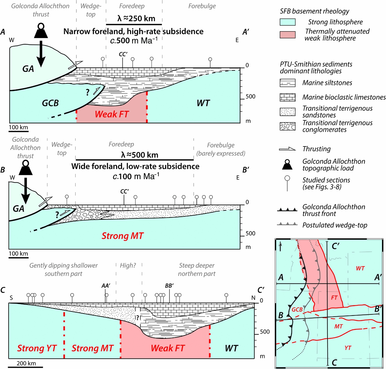
Figure 15. Cross-sections of the Sonoma Foreland Basin (SFB) illustrating variations in the subsidence and sedimentary accumulation pattern during the PTU-Smithian interval. The Golconda Allochthon (GA) is the main topographic load on the lithosphere (Dickinson, Reference Dickinson2006, Reference Dickinson2013; Marzolf, Reference Marzolf, Dunn and McDougall1993); the postulated wedge-top is also represented. (AA’) W–E cross-section in the northern part of the basin exhibiting a narrow foreland with a high-rate tectonic subsidence with a developed silty and limestone sedimentation over the Mesoproterozoic ‘thermally attenuated weak’ Farmington Terrane (FT). (BB’) W–E cross-section in the southern part of the Sonoma Foreland Basin showing a wide foreland with a low-rate tectonic subsidence, forming a reduced deposition of mainly terrigenous clastic series upon the Palaeoproterozoic ‘strong’ Mojave Terrane (MT). A barely expressed forebulge borders this part of the SFB. (CC’). S–N cross-section of the basin, highlighting the differences between southern and northern parts of the SFB in terms of subsidence, sedimentation and geometry of the basin. The transition between these two parts is situated close to the terranes boundary between MT and FT. This area is postulated to be a basement topographic highland, as supported by the transition between southern terrigenous clastic series and northern silty sedimentation.
Combining all field data and numerical simulations, a model of the SFB is proposed in Figure 15. The northern part of the basin (section AA’) is characterized by a narrow foredeep (λ ≈ 250 km) with a high-rate tectonic subsidence (c. 500 m Ma–1) and high sedimentary thickness (up to c. 550 m of mostly fine siltstones deposits), which is located upon the ‘weak/attenuated’ Farmington Terrane and in front of the largest reconstructed part of the GA. The postulated wedge-top and forebulge are located above the ‘strong’ Archean lithospheres, that is, the GCB and WT, respectively. The southern part of the SFB exhibits a large foredeep (λ ≈ 500 km, section BB’) with a relatively low-rate tectonic subsidence (c. 100 m Ma–1) and a reduced sedimentary thickness (up to c. 250 m of mixed limestones and coarse clastic deposits). This part of the SFB is emplaced upon the ‘strong’ lithospheres of the Palaeoproterozoic MT and YT, in front of the thinnest reconstructed part of the GA. The southern SFB also shows a reduced postulated wedge-top to the west and a barely expressed forebulge to the east. These spatial variations in flexural subsidence and their good agreement with limits of the terranes composing the SFB basement are also evident along a S–N transect (section CC’). The spatial separation between the shallow and gently dipping southern part of the SFB and the deep and steep northern part is obvious. This separation is located close to the boundary between MT and FT.
6. Conclusion
In this study, we used an integrated approach to decipher the major role of the lithospheric heritage over the differential sedimentary deposition in the Sonoma Foreland Basin during Early Triassic time. Our approach used both field-based sedimentary data, calibrated within a highly resolved biostratigraphic framework, and numerical model to test the influence of several potential controlling factors. Palinspastic reconstructions were also performed to obtain an accurate palaeogeographic context.
Using high-resolution temporal data, the subsidence analyses help to identify the main controlling factors at the origin of the spatial variations of the Early Triassic sedimentary record in the SFB. The sedimentary overload cannot satisfactorily explain the observed variations in thickness of the sedimentary record throughout the basin. The combined effects of the contrasted lithospheric strength of the terranes (‘weak’ v. ‘strong’ lithospheres) composing the basement of the basin, and the spatial heterogeneity of the Golconda Allochthon (with the presence of a lateral ramp within the belt), best explain a differential flexural response of the SFB basement to the emplacement of the allochthon. Such a differential flexural response ultimately controls the overall geometry of the basin through spatially heterogeneous tectonic subsidence rates: c. 100 m Ma–1 in a wide southern part upon a ‘strong’ lithosphere loaded by a recessed and thin (in map-view) front belt, v. c. 500 m Ma–1 in a narrower northern part upon a ‘weak/attenuated’ lithosphere loaded by a larger front belt. Although field data highlight the potential role of the rheological behaviour of the basement based on observed differential subsidence rates, the numerical model approach suggests a combined effect of the latter and of the spatial heterogeneity of the allochthon.
As heterogeneities of the basement and in the morphology of the allochthon result from the nature and history of the different lithospheric terranes that compose the basement, the lithosphere heritage likely played a prime role in controlling the development of the Sonoma Foreland Basin during Early Triassic time, and consequently generated the observed variations of the sedimentary record through differential subsidence.
Acknowledgements
We particularly thank the late Professor W.R. Dickinson for constructive discussions. We also thank Hugo Bucher and Romain Jattiot (Zürich) for discussion on Nevada outcrops. This work is a contribution to the ANR project AFTER (ANR-13-JS06-0001-01). The study was also supported by ENGIE.
Supplementary material
To view supplementary material for this article, please visit https://doi.org/10.1017/S0016756817000164.


