What drives conditional cooperation in public good games?

Peter Katuščák; Tomáš Miklánek

doi:10.1007/s10683-022-09756-9

What drives conditional cooperation in public good games?

Published online by Cambridge University Press: 14 March 2025

Peter Katuščák and

Tomáš Miklánek

Show author details

Peter Katuščák*: Affiliation:
School of Business and Economics, RWTH Aachen University, Templergraben 64, 52064 Aachen, Germany
Tomáš Miklánek: Affiliation:
Prague University of Economics and Business, Faculty of Business Administration, W. Churchill Sq. 4, 130 67 Prague 3, Czech Republic
*: Peter.Katuscak@vwl1.rwth-aachen.de

Article contents

Abstract
Introduction
Related literature
Experimental design and identification strategy
Methodology for data analysis
Results
Robustness in a between-subject design
Discussion
Conclusion
Funding
Footnotes
References

Rights & Permissions

Abstract

Extensive experimental research on public good games documents that many subjects are “conditional cooperators” in that they positively correlate their contribution with (their belief about) contributions of other subjects in their peer group. The goal of our study is to shed light on what preference and decision-making patterns drive this observed regularity. We consider reciprocity, conformity, inequality aversion and residual factors, such as confusion and anchoring, as potential explanations. Effects of these drivers are separated by varying how others’ contributions are determined and the informational content of the conditioning variable across treatments. Assuming additive separability of the effects of the four drivers, we find that, of the average conditionally cooperative behavior, at least 40 percent is driven by residual factors. For the remainder, most is accounted for by inequality aversion, some by conformity and very little by reciprocity. These findings carry an important message for how to interpret conditional cooperation observed in the lab. We also discuss what these findings mean for understanding conditional cooperation in fundraising applications in the field.

Keywords

Conditional cooperation Reciprocity Conformity Inequality aversion Confusion Anchoring

JEL classification

D64: Altruism • Philanthropy • Intergenerational Transfers H41: Public Goods C91: Laboratory, Individual Behavior

Type: Original Paper
Information: Experimental Economics , Volume 26 , Issue 2 , April 2023 , pp. 435 - 467

DOI: https://doi.org/10.1007/s10683-022-09756-9 [Opens in a new window]
Creative Commons: This is an Open Access article, distributed under the terms of the Creative Commons Attribution (CC-BY) license (http://creativecommons.org/licenses/by/4.0/), which permits unrestricted re-use, distribution, and reproduction in any medium, provided the original work is properly cited.
Copyright: Copyright © The Author(s) 2022

1 Introduction

Casual observation as well as an extensive experimental literature (Ledyard, Reference Ledyard, Kagel and Roth1995) document that people voluntarily contribute to public goods. This observation is squarely at odds with the traditional model of self-regarding preferences. Under this model, each individual has a strictly dominant strategy of free-riding (i.e., contributing zero). Most of the existing explanations of this empirical regularity rely on existence of social preferences.Footnote ¹ Although positive voluntary contributions can be explained by maximization of social welfare (Laffont Reference Laffont1975) or altruistic/warm-glow preferences (Becker, Reference Becker1974; Andreoni, Reference Andreoni1989, Reference Andreoni1990), predictions of these theories within the linear public good game, a workhorse of research in this area, do not square well with empirical evidence. In particular, while these theories predict that an individual contributes the same amount no matter how much the others contribute, Fischbacher et al.,, (Reference Fischbacher, Gächter and Fehr2001) (henceforth FGF) document that a sizable group of subjects contribute more if the others on average contribute more as well. They call this empirical pattern “conditional cooperation” (henceforth CC). The authors classify about one half of their subjects as conditional cooperators (henceforth CCs), one third as free-riders (contributing zero regardless of the average contribution of the other group members), and the rest as fitting other (or no particular) patterns. These findings have later been replicated by numerous laboratory studies (Thöni & Volk, Reference Thöni and Volk2018). Moreover, multiple studies in the labFootnote ² and in the fieldFootnote ³ document a positive correlation between contributions and historical contributions or beliefs about current contributions of others, suggesting presence of CC.

It is not very well understood, however, what preference and decision-making patterns drive CC and what their relative roles are. CC could be driven by reciprocity (to perceived intentions behind others’ contributions), conformity (to others’ contributions regardless of payoff consequences), aversion to payoff inequality (in comparison to others regardless of their intentions), and other residual factors. Reciprocity is a kind (unkind) response to an action by others that is perceived to be driven by their kind (unkind) intention (Rabin, Reference Rabin1993; Dufwenberg & Kirchsteiger, Reference Dufwenberg and Kirchsteiger2004; Falk & Fischbacher, Reference Falk and Fischbacher2006) or by their generous (ungenerous) type (Levine, Reference Levine1998; Rotemberg, Reference Rotemberg2008; Gul and Pesendorfer, Reference Gul and Pesendorfer2016). Conformity is an act of following an observed behavior of others. It could arise due to adherence to a (perceived) social norm (Axelrod Reference Axelrod1986; Bernheim, Reference Bernheim1994; Fehr & Fischbacher, Reference Fehr and Fischbacher2004, a.k.a. “normative conformity”) or due to social learning about an optimal decision (Bikhchandani et al., Reference Bikhchandani, Hirshleifer and Welch1998, a.k.a. “informational conformity”). Inequality aversion is a willingness to take action in order to reduce material payoff inequality between oneself and others irrespective of whether the inequality originates from intentions of the others or not (Fehr & Schmidt, Reference Fehr and Schmidt1999; Bolton & Ockenfels, Reference Bolton and Ockenfels2000). Residual factors include any other alternative explanation of CC.

Regarding the residual factors, we speculate that the most important ones include anchoring and confusion. Anchoring is an act of letting one’s decisions be influenced by payoff- and belief-irrelevant numerical cues (Tversky & Kahneman, Reference Tversky and Kahneman1974). (Subject) confusion (Andreoni, Reference Andreoni1995; Keser, Reference Keser1996; Houser & Kurzban, Reference Houser and Kurzban2002) can be thought of as an imperfect “game form recognition” (Chou et al., Reference Chou, McConnell, Nagel and Plott2009) in that subjects fail to properly understand how players’ strategy combinations map to their payoffs and, consequently, fail to recognize what would constitute an optimal strategy given one’s own preferences.Footnote ⁴ The possibility that laboratory-observed CC is driven by confusion has been illustrated by Ferraro and Vossler (Reference Ferraro and Vossler2010) and Burton-Chellew et al., (Reference Burton-Chellew, El Mouden and West2016). These two studies find that when subjects play the public good game against computers using the FGF design, with nobody else benefiting from their contributions, the classification into conditional contribution types results in a distribution remarkably similar to that of FGF and its replications. In particular, the share of CCs is approximately 50%. All this happens despite subjects having to answer control questions that are supposed to assure understanding of the instructions. Moreover, Burton-Chellew et al., (Reference Burton-Chellew, El Mouden and West2016) document that CCs, as opposed to free-riders, are more likely to misunderstand the game.

Knowing more about the relative strength of the four potential drivers, apart from being interesting on its own, has important implications for how to interpret, extrapolate, and, in a fundraising setting, also exploit empirical findings on CC. Traditionally, CC has been approached as an all-encompassing reflection of cooperative behavior or, at a more granular level, as a reflection of reciprocity, inequality aversion or conformity. In the laboratory setting, however, this view has been challenged by the results of Ferraro and Vossler (Reference Ferraro and Vossler2010) and Burton-Chellew et al., (Reference Burton-Chellew, El Mouden and West2016). The latter go as far as to suggest that laboratory-observed CC might, in essence, be a data pattern driven purely by confusion. Given the prominence of the FGF method in measuring CC, it is important to shed more light on the role that confusion (and anchoring) play in such measurement. In the fundraising field setting, understanding the relative role of various drivers of CC is likely to be useful for choosing the type of “social information” to be presented to would-be contributors. If CC is driven by conformity, then behavior of any present or historical reference group of contributors can be used to motivate higher contributions.Footnote ⁵ If CC is driven by reciprocity, it might be necessary to refer to a group of earlier contributors in the current fundraising campaign instead. If CC is driven by fairness concerns (i.e., inequality aversion), it is important to carefully consider which reference groups (for example, income- or wealth-wise) would be most relevant to would-be contributors. If CC is driven by anchoring, suitably suggesting a contribution amount might be all that is required.

The aim of our study is to disentangle the four potential drivers of CC in a laboratory setting. We utilize a modified version of the FGF design (detailed in Sect. 3). In a within-subject design, each subject, after contributing unconditionally (treatment 1), is also faced with four conditional contribution treatments. In treatments 2 to 4, subjects condition on the average contribution of the three other members of their contribution group. What differs across these three treatments is how the contributions of the other three group members are determined. In treatment 2, the other group members’ contributions are equal to their unconditional contributions from treatment 1, as in the original design of FGF. All four explanations play a potential role here. In treatment 3, the other group members’ contributions are equal to unconditional contributions of three randomly chosen group non-members from treatment 1. This treatment eliminates reciprocity as an explanation of CC because the conditioning variable no longer reflects intentions of the other group members.Footnote ⁶ In treatment 4, the other group members’ contributions are randomly generated by computer. On top of treatment 3, this treatment also eliminates conformity as an explanation. Finally, in treatment 5, subjects no longer condition on the average contribution of the three other members of their contribution group, but, rather, they condition on the average of three randomly drawn numbers that are independent of the groupmates’ contributions. The other group members’ contributions are independently randomly generated by the computer. On top of treatment 4, this treatment eliminates also inequality aversion and leaves only residual factors as a potential explanation. We identify the impact of reciprocity by comparing conditional contributions in treatments 2 and 3; that of conformity by comparing treatments 3 and 4; that of inequality aversion by comparing treatments 4 and 5. Treatment 5 identifies the impact of residual factors.

We do not attempt to separate anchoring from confusion as it is inherently difficult. Whenever anchoring is present, some type of confusion is very likely to be present as well.Footnote ⁷ Whenever confusion is present, there are some ex post patterns of conditional contributions that would allow one to argue that anchoring is not present.Footnote ⁸ However, it is hard to think of a reliable way to rule out anchoring by design ex ante.

Based on the within-subject design, we find a strong CC behavior even in treatment 5 in which only the residual factors play a role. Adding inequality aversion in treatment 4 further increases the extent of CC behavior. Adding conformity in treatment 3 leads to a small further increase in CC behavior with borderline statistical significance. Finally, adding reciprocity in treatment 2 has a minimal impact on CC behavior. Based on the estimated slopes of the average conditional contribution schedules by treatment, we find that residual factors account for about two thirds, inequality aversion for one quarter and conformity for one tenth of the CC behavior. Reciprocity is estimated to play virtually no role.

Next, we examine robustness of these findings to a possible imperfect perception of various treatments and their differences created by the within-subject design and presentation of the instructions. For this purpose, we collect additional data for treatments 2 and 5 using a between-subject design. Based on the estimated slopes of the average conditional contribution schedule by treatment, we find that residual factors account for about 59% of the CC behavior. If restricting the sample to only those who demonstrate a strong understanding of the instructions, the share is 45%. This robustness check therefore confirms the important role of residual factors in driving conditionally cooperative behavior in treatment 2.

The paper proceeds as follows. Section 2 reviews the related literature. Section 3 outlines the experimental design. Section 4 reviews the utilized empirical methodology. Section 5 presents our results. Section 6 presents the design and results of the robustness analysis based on the between-subject design. Section 7 links the findings to the previous literature and discusses a potential alternative explanation of the results in treatment 5. Finally, Sect. 8 concludes.

2 Related literature

2.1 Reciprocity, conformity, inequality aversion and anchoring

This study is most closely related to the work of Bardsley and Sausgruber (Reference Bardsley and Sausgruber2005) and Cappelletti et al., (Reference Cappelletti, Güth and Ploner2011). Bardsley and Sausgruber (Reference Bardsley and Sausgruber2005) attempt to distinguish the roles of reciprocity and conformity in driving CC. They analyze conditional contribution behavior of subjects who see possible vectors $x_{- i}$ of contributions of other members of their own group and possible vectors y of members of another group. They identify conformity by reaction to changes in y, holding $x_{- i}$ constant. They identify the combined CC effect of reciprocity and conformity by reaction to changes in $x_{- i}$ , holding y constant. Assuming additive separability of the two drivers, they conclude that, of the combined effect, 2/3 are accounted for by reciprocity and 1/3 is accounted for by conformity. This identification strategy requires that the strength of conformity with $x_{- i}$ and that with y is the same. However, this is unlikely to be the case given the utilized design. The issue is that all the members of the own group, even those who account for $x_{- i}$ , see y before deciding on their contributions. As a result, especially in cases when the level of contributions in $x_{- i}$ and y is very different, it is reasonable to expect that conformity with $x_{- i}$ is stronger than that with y because the decision-maker is likely to infer that if the other group members chose to deviate from the level of contributions in y, there is probably a good reason to do so (informational conformity). Indeed, this reasoning appears to be confirmed by the data.Footnote ⁹ As a result, the estimate of 1/3 of the total CC effect is likely to be an underestimate of the true effect of conformity in the combined effect of conformity and reciprocity. Also, the paper does not attempt to experimentally isolate the roles of inequality aversion and residual factors.

Cappelletti et al., (Reference Cappelletti, Güth and Ploner2011) attempt to disentangle the roles of reciprocity, inequality aversion and anchoring, but not that of conformity. They use a design that shares a similarity with FGF in terms of eliciting conditional contributions, but differs from it by making payoffs non-linear in contributions (with a strictly increasing marginal cost of contributions) and using repeated play based on a stranger-matching protocol. They find that CC behavior is predominantly driven by anchoring and inequality aversion (by about the same amount), with reciprocity having a small and statistically marginal role.Footnote ¹⁰^, Footnote ¹¹^, Footnote ¹²

Our design attempts to integrate the existing approaches in a broader and unified framework. First, we consider all four potential drivers of CC behavior in a single setting. Second, our design builds on the FGF design that uses a linear public good game and that is also used in many existing replications (Thöni & Volk, Reference Thöni and Volk2018). This makes our study directly comparable to many other studies in the literature. Third, our conditioning variable is always the average of three independent unconditional contributions or randomly drawn numbers. We hence avoid information-cascade-like problems in interpreting various conditions.

Other authors have attempted to address similar questions using data from repeatedly-played public good games. Ashley et al., (Reference Ashley, Ball and Eckel2010) attempt to distinguish the roles of reciprocity and inequality aversion, but not those of conformity or other factors, using data from repeated public good game experiments with fixed-group matching and ex post observability of individual contributions in the previous period within own group only (baseline treatment) or also across groups (alternative treatment). They conclude that the dynamics of contributions are more consistent with inequality aversion than with reciprocity. However, the fixed-group design with repeated interaction allows for alternative interpretations of the results based on dynamic strategizing and reputation-building.Footnote ¹³^, Footnote ¹⁴

2.2 Confusion

As discussed in Sect. 1, subject confusion might play a significant role in explaining laboratory-observed CC. Burton-Chellew et al., (Reference Burton-Chellew, El Mouden and West2016) list several reasons they think lead to subject confusion in the original FGF design: (1) using the verb “invest” to describe the act of contribution might invoke a sense of a risky endeavor the return to which depends on complementary “investment” of others; (2) subjects might not be fully aware of the private cost of contributing and hence might not realize the social dilemma that they face; for example, of the four control questions aimed at assuring understanding, only one (question 3) illustrates the trade-off inherent in the social dilemma; (3) since asked to contribute conditionally, subjects might think that the value of the conditioning variable is important and that their conditional contribution should vary with it even though they cannot see an obvious reason for such correlation (an experimenter demand effect).Footnote ¹⁵ Goeschl & Lohse, (Reference Goeschl and Lohse2018) and Recalde et al., (Reference Recalde, Riedl and Vesterlund2018) argue and document that confusion in public good games might be aided by time pressure. We use these suggestions as a guideline for our experimental design. We develop an alternative set of instructions that uses the verb “contribute” instead of “invest” to describe the act of contribution. Instead of using control questions, which both Ferraro & Vossler, (Reference Ferraro and Vossler2010) and Burton-Chellew et al., (Reference Burton-Chellew, El Mouden and West2016) find to be ineffective in preventing confusion, we aid understanding of the game by giving subjects an opportunity to simulate their and other group members’ payoffs on a simulator (see Section 3). The simulator gives subjects a simple interface to perform a ceteris paribus analysis of how a marginal change in their or another subject’s contribution affects payoffs of all members of the group. Also, we remove any time pressure from subjects and let them proceed at their own pace.

More generally, instead of merely examining a potential presence of confusion in conditional contributions, our study integrates confusion into a fully-fledged CC decomposition exercise. Moreover, unlike Ferraro and Vossler (Reference Ferraro and Vossler2010) and Burton-Chellew et al., (Reference Burton-Chellew, El Mouden and West2016), which rely on subjects interacting with computerized players, all players in our design are humans. As a result, we avoid a criticism raised against the two studies that their findings are driven by subjects being uncertain about who, if anyone, collects the payoffs.

3 Experimental design and identification strategy

We build on the original design of FGF with some modifications. Subject play a linear public good game in groups of four. Each subject i independently decides how many of her 10 tokens (as opposed to 20 in FGF) to allocate into her private account ( $10 - g_{i}$ ) and how many to contribute (as opposed to “invest” in FGF) to a “group project” ( $g_{i}$ ). Each subject receives a payoff from the public good equal to 0.75 (instead of 0.4 in FGF) times the sum of all the contributions to the group project. Hence the material payoff in tokens of subject i is given by $π_{i} = 10 - g_{i} + 0.75 \sum_{j = 1}^{4} g_{j}$ , where j indexes the members of the same contribution group. The reason why we use the marginal per capita return of 0.75 instead of 0.4 is to secure a high share of CCs in order to increase statistical power of our decomposition exercise.

Subjects make contribution decisions in five different treatments, labeled to them as “scenarios,” described in Sect. 3.2. The underlying public good game is the same across all five treatments and subjects are informed that any decision they make in the experiment has a positive chance of being payoff-relevant for them and the other group members.

3.1 Procedure

Each experimental session begins with one-page printed General Instructions (see Online appendix A). Subjects are given information about the outline of the experiment, including the number of treatments, the fact that they will not be given any feedback on their or anyone else’s decisions or earnings before a feedback stage at the end of the experiment. They are also informed about the exchange rate between experimental tokens and cash. Finally, they are also informed that in each treatment they will interact in groups of 4 subjects and that everyone will be paid based on the same one treatment (strategy method) randomly determined by a public draw at the end of the experiment. This is followed by another one-page printed instructions (see Online appendix A) describing the public good game and its payoffs. This is the game played in treatment 1. Subjects are also notified that payoffs are calculated in the same way also in the following four treatments.

Subjects then get 3 minutes to interact with an on-screen simulator (see Figure B1 in Online appendix B for a screenshot) using which they can simulate their earnings and the earnings of the other group members as a function of all four group members’ contributions. Initial simulated values of the four contributions are randomly selected by computer in order to mitigate any potential anchoring bias. Subjects can add to or subtract from the individual contributions in the increments of 1 token. After each such incremental change, subjects can observe the change in everyone’s payoffs. The design of the simulator aims to clarify to subjects what the marginal payoff consequences of their own contribution and of the other group members’ contributions are. Afterwards, the experiment progresses to treatment 1 in which subjects decide on their unconditional contributions (see Figure B2 in Online appendix B for the input screen).

After treatment 1 is finished, we distribute additional printed instructions that are common to treatments 2-5 (see Online appendix A) which are labeled as “conditional treatments.” They explain the principle of conditional contributions as follows. There are three “Type X” participants and one “Type Y” participant in each group. Types of all subjects are chosen by computer at the end of the experiment, with each participant in a group having the same chance of being the Type Y participant. The Type X participants contribute to the public good according to the rule announced for each treatment. The Type Y participant contributes to the public good based on his/her decisions in the “contribution table.” In this table, subjects specify how much they wish to contribute conditionally on the rounded average of three numbers. Subjects are told that what these numbers are will be announced to them at the beginning of each treatment. The conditioning variable takes values from the set ${0, 1, . . ., 10}$ . The task in each treatment is to specify the conditional contribution for each possible value of the conditioning variable for the case one is selected to be the Type Y participant. The instructions then describe what the contribution table looks like and, by means of examples, which input into the contribution table becomes relevant for the group members’ earnings. Subjects are also told that treatments 2-5 will be presented to them in a random order and that they will receive instructions for each treatment on the screen.

Subjects are then sequentially presented with treatments 2-5 in a scrambled order (see Online appendix A for on-screen instructions) and make 11 conditional contribution decisions in each treatment (see Figures B3-B6 in Online appendix B for the input screens in treatment 2-5). Subjects are never aware of the content of the upcoming treatments while making their decisions for the current treatment. The on-screen instructions and the input screens inform subjects about how the actual contributions of the three Type X participants are determined and about the definition of the conditioning variable. In order to further aid understanding, the text instructions are complemented by graphical schemes illustrating how the contributions are determined in that particular treatment (see Online appendix A).Footnote ¹⁶

After all subjects have finished entering their conditional contributions, we administer a demographic questionnaire. We elicit gender, age, country of origin, number of siblings, academic major, the highest achieved academic degree so far, and an estimate of monthly spending.

Subjects are paid based on their decisions in one treatment chosen randomly by a public draw of a chip from a set of chips numbered 1 to 5 at the end of the experiment. If treatment 1 is chosen to be payoff-relevant, the contributions are determined according to the decision of each group member in that treatment. If one of the other four conditional treatments is chosen to be payoff-relevant, then one group member is randomly chosen by computer to be the Type Y participant, with the remaining three group members being assigned the role of Type X participants. Everyone’s contributions and earnings are then determined according to the rules described above. At the end of the experiment, experimental earnings in tokens are converted into cash and paid privately to subjects.

3.2 Treatments

In treatment 1, subjects simply decide how much to contribute unconditionally. This treatment is the first treatment presented to all subjects. This treatment is followed by four conditional treatments. They differ in two respects. First, in treatment 2, as in FGF, the groupmates’ contributions are equal to their unconditional contributions from treatment 1. In treatment 3, the groupmates’ contributions are equal to unconditional contributions of three randomly chosen group non-members from treatment 1. In treatment 4 and 5, the groupmates’ contributions are randomly and independently generated by computer from the uniform distribution on ${0, 1, . . ., 10}$ . Second, in treatments 2, 3 and 4, the conditioning variable is equal to the rounded average contribution of the three other group members in that treatment. In treatment 5, it is equal to the rounded average of three randomly and independently drawn numbers from the uniform distribution on ${0, 1, . . ., 10}$ that are independent from the groupmates’ contributions.Footnote ¹⁷^, Footnote ¹⁸

3.3 Identification strategy

This design allows us to disentangle the impact of reciprocity, inequality aversion, conformity and residual factors on the conditional contribution behavior in treatment 2. Behavior in this treatment is potentially affected by all four drivers. To outline the argument, note that, ceteris paribus, each additional token contributed by members 2, 3 and 4 on average increases $π_{1}$ by 2.25 tokens and $π_{j}$ , for $j \in {2, 3, 4}$ , by 1.25 tokens. This has two implications. First, an additional token of ${\bar{g}}_{234}$ might be viewed by member 1 as a kind marginal act of her groupmates toward herself, triggering intention-based reciprocity.Footnote ¹⁹ Alternatively, it might be seen by member 1 as a marginal signal of the groupmates’ generosity, triggering an increased generosity by member 1 herself within the context of interdependent-type reciprocity. In either case, the resulting reciprocity increases $g_{1}$ . Second, member 1 might take a normative or an informational cue from ${\bar{g}}_{234}$ . If so, an additional token of ${\bar{g}}_{234}$ increases $g_{1}$ by conformity. Third, an additional token of ${\bar{g}}_{234}$ increases the payoff of member 1 relative to her groupmates by 1 token on average. If averse to payoff inequality, member 1 will counteract such increase by increasing $g_{1}$ . Fourth, if member 1 is unsure about what conditional contributions to pick, ${\bar{g}}_{234}$ might serve as an anchor and hence $g_{1}$ will be positively correlated with ${\bar{g}}_{234}$ .

Treatments 3, 4 and 5 eliminate reciprocity as a driver since contributions of the groupmates are not determined by themselves. As a result, the conditioning variable does not carry any information about groupmates’ intentions or generosity types. Treatments 4 and 5 also eliminate conformity as a driver since the conditioning variable is computer-generated and hence does not carry information about any human decisions. Treatment 5 in addition eliminates inequality aversion as a driver since the conditioning variable does not carry any useful information. The identification strategy is summarized in Table 1. Assuming additive separability among the impacts of the four drivers, the impact of reciprocity is identified by differencing conditional contributions between treatments 2 and 3; that of conformity by differencing between treatments 3 and 4; and that of inequality aversion by differencing between treatments 4 and 5. Treatment 5 identifies the impact of residual factors. This way, the conditional contribution behavior in treatment 2 can be decomposed into the four components corresponding to the four respective behavior drivers.

Table 1 Presence of behavior drivers in the four treatments

	Treatment 2	Treatment 3	Treatment 4	Treatment 5
Reciprocity	×
Conformity	×	×
Inequality aversion	×	×	×
Residual factors	×	×	×	×

Some discussion is in order before proceeding. First, regarding a potential confound in treatment 3, although subjects cannot directly reciprocate to the subjects whose intentions lie behind the groupmates’ contributions, they might “generally” reciprocate to other subjects. If so, behavior in treatment 3 might be driven by “generalized” reciprocity to some extent.Footnote ²⁰ Distinguishing generalized reciprocity from conformity is difficult in lab conditions under anonymity and random assignment of subjects to groups or roles. Hence, to the extent it is present, we subsume generalized reciprocity under the “conformity” label.

Second, regarding another potential confound, to the extent that a higher ${\bar{g}}_{234}$ in treatment 2 might come hand-in-hand with a higher second-order belief of the conditional contributor about how much her groupmates expect their groupmates to contribute,Footnote ²¹ an increasing conditional contribution schedule could (partly) be driven by guilt aversion (Charness & Dufwenberg, Reference Charness and Dufwenberg2006; Battigalli & Dufwenberg, Reference Battigalli and Dufwenberg2007) instead of reciprocity. Some previous studies have tried to induce exogenous variation into second-order beliefs while keeping material payoffs constant and the results are inconclusive (Ellingsen et al., Reference Ellingsen, Johannesson, Tjøtta and Torsvik2010; Al-Ubaydli and Lee Reference Al-Ubaydli and Lee2012; Engler et al., Reference Engler, Kerschbamer and Page2018). Since we want to stay close to the FGF design blueprint, we do not elicit and manipulate beliefs and therefore have no way of distinguishing the two drivers. In our setting, they arguably work in the same direction, so we will subsume guilt aversion under the “reciprocity” label.

Third, when it comes to reciprocity, conformity and inequality aversion, the conditional contributor can only condition on the rounded average contribution of the other group members. The conditional contributor does not get to see what three contributions are behind this rounded average. This is potentially limiting since the conditional contributor might prefer to use another reference point than the average when expressing his preferences. We therefore need to assume that the rounded average is a sufficient statistic for expressing one’s preferences.Footnote ²²

Fourth, we opt for a within-subject design as opposed to a between-subject design because of noise reduction. Previous studies point to a significant heterogeneity in conditional contribution behavior among subjects in the FGF design across many different populations.Footnote ²³ Anticipating such heterogeneity also in our subject population, the within-subject design reduces the resulting noise in the estimates of the impact of the various behavior drivers. In order to mitigate impact of potential treatment order effects on our inference, we evenly balance all 24 possible orderings of the four conditional treatments in the sample.

3.4 Logistics

We collected data for 192 subjects over 9 sessions. There are 8 participating subjects for each of the 24 orders in which the four conditional treatments were presented. Due to a technical problem, the decisions of one subject for one of the scenarios were not recorded. Given our emphasis on within-subject design, we decided to drop this subject from our data set. The dataset we utilize therefore contains 191 subjects. All sessions were conducted in the Laboratory of Experimental Economics (LEE) at the University of Economics in Prague in May and June 2018. The experiment used a computerized interface programmed in zTree (Fischbacher Reference Fischbacher2007). Subjects were recruited using the Online Recruitment System for Economic Experiments (Greiner, Reference Greiner2015) from a subject database of the lab. Our subjects are students from various universities in Prague, mostly from the University of Economics. Almost 72% of the subjects report “Economics or Business” as their field of study. The gender ratio is almost exactly balanced.Footnote ²⁴ One experimental token was worth 10 Czech koruna (CZK).Footnote ²⁵ The mean and median cash payoff, including a CZK 75 show-up fee, was CZK 280Footnote ²⁶ for approximately 1 hour of participation.Footnote ²⁷

4 Methodology for data analysis

We use two different methods to examine what drives CC. The first method is based on the average conditional contributions given each value of the conditioning variable. This method estimates the slope of the average conditional contributions in the value of the conditioning variable in treatment 2 and decomposes this slope into analogous slopes due to the four constituent drivers. The second method classifies subjects into types according to the pattern of their conditional contributions in a given treatment. It then traces how the type distribution changes across different treatments and what that reveals about the four constituent drivers of CC.

4.1 Slope decomposition

Formally, let i index subjects, $j \in {2, 3, 4, 5}$ index the conditional treatments and $c \in {0, 1, . . ., 10}$ index the value of the conditioning variable. Let $g_{ijc}$ be the conditional contribution of subject i in treatment j if the value of the conditioning variable is c. Then the extent to which average conditional contributions increase with c in the given treatment can be estimated by the slope coefficient in the regression

(1)

\begin{matrix} g_{ijc} = α_{j} + β_{j} c + u_{ijc} . \end{matrix}

With ${\hat{β}}_{2}$ being the OLS estimate of $β_{2}$ , the extent of CC can then be measured by ${\hat{β}}_{CC} \equiv {\hat{β}}_{2}$ . Using the identification strategy presented in Subsect. 3.3, the extent of CC attributable to the four drivers can be estimated by ${\hat{β}}_{R} \equiv {\hat{β}}_{2} - {\hat{β}}_{3}$ for reciprocity, ${\hat{β}}_{C} \equiv {\hat{β}}_{3} - {\hat{β}}_{4}$ for conformity, ${\hat{β}}_{IA} \equiv {\hat{β}}_{4} - {\hat{β}}_{5}$ for inequality aversion and ${\hat{β}}_{RF} \equiv {\hat{β}}_{5}$ for residual factors. By construction, we then have that

(2)

\begin{matrix} {\hat{β}}_{CC} = {\hat{β}}_{R} + {\hat{β}}_{C} + {\hat{β}}_{IA} + {\hat{β}}_{RF} . \end{matrix}

This equation describes the slope decomposition. We estimate all the coefficients in one regression with treatment interactions for intercept and slope. When computing standard errors and performing statistical tests, we use clustering at subject level.

4.2 Subject type classification

The slope decomposition at the sample level that we described in the previous subsection can also in principle be done at the individual level. However, each such coefficient estimate is then based on only 11 conditional contributions of one subject in question. Given the small sample size and a lack of independence, no statistically meaningful conclusions can be drawn about such coefficients using conventional statistical methods.

In order to gain at least some insight into subject heterogeneity, we turn to the classification method of Thöni & Volk, (Reference Thöni and Volk2018), which is itself a slight modification of the method used by FGF. Given the power difficulty mentioned in the previous paragraph, instead of capturing the extent of CC quantitatively, this method focuses on qualitatively distinguishing various types of conditional contribution schedules. The method distinguishes five conditional contribution patterns. In particular, a subject is classified to be a: (1) conditional cooperator if $g_{i 2 c}$ is weakly monotonically increasing in c without being flat in c, or the estimated Pearson correlation coefficient between $g_{i 2 c}$ and c is at least 0.5; (2) free-rider if $g_{i 2 c} = 0$ for all c; (3) unconditional cooperator if $g_{i 2 c} = g > 0$ for all c; (4) “triangle cooperator” if there is a value $\bar{c} \in {1, . ., 9}$ such that $g_{i 2 c}$ is weakly monotonically increasing on $c \in {0, . ., \bar{c}}$ and weakly monotonically decreasing on $c \in {\bar{c}, . ., 10}$ , without being flat in c in either of the two regions, or there is a value $\bar{c} \in {2, . ., 8}$ such that the Pearson correlation coefficient between $g_{i 2 c}$ and c is at least 0.5 for $c \in {0, . ., \bar{c}}$ and at most $- 0.5$ for $c \in {\bar{c}, . ., 10}$ ; (5) other if subject i is not classified as any of the previous four types. Moreover, if it happens that subject i satisfies the conditions for being both a CC and a triangle cooperator, then the subject is classified as a CC if and only if $g_{i 2 10} > \frac{1}{11} \sum_{c = 0}^{10} g_{i 2 c}$ .

We extend this methodology from treatment 2 to all four conditional treatments. This way we can estimate the distribution of types in each treatment and examine how it shifts across treatments. In doing so, we pay special attention to how the share of CCs shifts across the four treatments.

5 Results

5.1 Preliminary analysis

Figure 1 presents a histogram of unconditional (i.e., treatment 1) contributions. The mean (median) unconditional contribution is 6.13 (6) out of 10. This is at the upper boundary of the range typically found in the literature (Ledyard, Reference Ledyard, Kagel and Roth1995). We attribute this finding to a MPCR of 0.75 that is also higher than what is usually found in the literature. A high MPCR makes contributing to the public good cheap and hence, for example, a given distribution of reciprocity or inequality aversion in the population leads to a higher level of unconditional contributions on average.

Fig. 1 Histogram of unconditional contributions

Figure 2 plots the average conditional contribution across all subjects by the value of the conditioning variable c and treatment (2 through 5). In treatment 2, we observe that that the pattern of conditional contributions is monotonically increasing with c, suggesting presence of CC. In particular, the average conditional contribution for $c = 10$ is by about 4.5 tokens larger than the average conditional contribution for $c = 0$ . This suggests that the extent of CC is quantitatively sizeable on average at almost one-half-for-one. The pattern of the average conditional contributions in treatment 3 is almost identical, suggesting that reciprocity plays little role in explaining CC. The pattern of the average conditional contributions in treatment 4 is also monotonically increasing with c. It is almost identical to treatments 2 and 3 for up to $c = 3$ , but it diverges from the previous two treatments downwards for higher values of c. At $c = 10$ , the gap is about 0.5 tokens. This suggests that conformity does play a role in explaining CC, albeit not a quantitatively very large one. The pattern of the average conditional contributions in treatment 5 is also increasing in c, but the slope is smaller than in treatment 4. The difference between the average conditional contributions at $c = 0$ and $c = 10$ is about 3 tokens, as opposed to about 4 tokens in treatment 4. This suggests that inequality aversion plays an important role in explaining CC. Finally, somewhat unexpectedly, the pattern of average conditional contributions is (almost) monotonically increasing with c also in treatment 5. The difference between the average conditional contributions at $c = 10$ and $c = 0$ is almost 3 tokens, two thirds of the analogous difference in treatment 2. This suggests that not only are residual factors present as a driver of CC, but they actually account for a major part of it.

Fig. 2 Average conditional contribution by value of the conditioning variable and treatment

5.2 Slope decomposition

Results of the slope decomposition along the lines of Eq. (2) are presented in Table 2. In the left panel, columns “Intercept” and “Slope” report estimates of the intercept and the slope, respectively, of the average conditional contribution schedule by treatment (Eq. 1). The right panel presents how ${\hat{β}}_{CC}$ decomposes into ${\hat{β}}_{R}$ , ${\hat{β}}_{C}$ , ${\hat{β}}_{IA}$ and ${\hat{β}}_{RF}$ , both in absolute and in proportional terms.Footnote ²⁸ In line with our preliminary observations in Fig. 2, we find that the average conditional contribution in treatment 2 increases with c at the rate of approximately one half (precisely ${\hat{β}}_{CC} = 0.495$ ). That is, we observe imperfect (slope less than 1) but sizeable (slope more than 0) CC. In treatment 3, ${\hat{β}}_{3}$ is 0.492, almost as high as ${\hat{β}}_{2}$ . As shown in the right panel, the resulting difference of 0.002 (after rounding) accounts for only $0.5 %$ of ${\hat{β}}_{CC}$ and is not statistically significant (t-test $p = 0.924$ ). That is, reciprocity plays little role in explaining CC. In treatment 4, ${\hat{β}}_{4}$ is 0.44, which is by 0.052 less than ${\hat{β}}_{3}$ ( $p = 0.082$ ). Translated into proportional terms, this means that conformity accounts for about one tenth of ${\hat{β}}_{CC}$ . In treatment 5, where only residual factors play a role, the slope estimate ${\hat{β}}_{5}$ drops to 0.322, which is by 0.118 less than ${\hat{β}}_{4}$ ( $p = 0.001$ ). In proportional terms, this implies that inequality aversion accounts for almost one quarter of ${\hat{β}}_{CC}$ . Finally, ${\hat{β}}_{5}$ is equal to 0.322, statistically significantly different from 0 ( $p < 0.001$ ). In proportional terms, residual factors account for almost two thirds ${\hat{β}}_{CC}$ .

Table 2 Estimated slope of the average conditional contribution schedule and its decomposition

To summarize the slope decomposition, the main driver of CC is the residual factors, accounting for approximately two thirds of CC. The second most important driver is inequality aversion, accounting for about a quarter of CC. Conformity accounts for approximately a tenth of CC, with the evidence for its presence being mildly statistically significant. Reciprocity plays virtually no role in driving CC.

5.3 Subject type classification

Table 3 displays a distribution of the conditional contribution type by treatment based on the method of Thöni & Volk, (Reference Thöni and Volk2018) (see subsection 4.2).Footnote ²⁹ In treatment 2, which corresponds to the setting considered in the previous literature, we classify 57.6% of subjects as conditional cooperators, 12.6% of subjects as triangle cooperators, 12.0% of subjects as free-riders, 9.4% of subjects as unconditional cooperators and 8.4% of subjects as having the “other” type. Regarding the incidence of CC and triangle cooperation, our results are consistent with the range of type distributions estimated in many previous studies (Thöni & Volk, Reference Thöni and Volk2018). Regarding the incidence of free-riding, our finding lies toward the bottom edge of the range identified in the literature. We speculate that this is primarily driven by a high MPCR of 0.75 in our study, which coincides with the upper boundary of the range used in the literature. Minimization of free-riding fits our objective of increasing the power of the CC decomposition analysis.

Table 3 Conditional contributor type classification by treatment (% of all subjects, shares of conditional cooperators in bolded)

	Treatment 2	Treatment 3	Treatment 4	Treatment 5
Conditional cooperator	57.6	56.0	52.9	40.8
Triangle cooperator	12.6	13.6	15.7	12.6
Free-rider	12.0	10.5	15.2	19.4
Unconditional cooperator	9.4	8.9	7.3	17.3
Other type	8.4	11.0	8.9	10.0

Looking beyond treatment 2, we observe that the type distribution in treatment 3 is almost identical to that in treatment 2, suggesting that reciprocity plays little role on average in driving conditional contribution behavior in treatment 2. This is confirmed by formal tests. Neither the type distribution (Stuart-Maxwell test $p = 0.546$ ), nor being classified as a CC (paired sign test $p = 0.690$ )Footnote ³⁰ is statistically significantly different across the two treatments. Moving on to treatment 4, there are some mild differences in the type distribution vis-à-vis treatment 3, such as a drop in the fraction of CCs from 56% to 52.9%. The difference in the type distribution is marginally statistically significant (Stuart-Maxwell test $p = 0.053$ ), but the difference in the fraction of CCs is not (paired sign test $p = 0.392$ ). This suggests that conformity plays at most a minor role in driving conditional contribution behavior in treatment 2. Moving on to treatment 5, there are relatively large differences in the type distribution vis-à-vis treatment 4. For example, there is a drop in the fraction of CCs from 52.9% to 40.8%. Both this difference (paired sign test $p = 0.003$ ) and the difference in the type distribution (Stuart-Maxwell test $p = 0.002$ ) are now statistically significant. This suggests that inequality aversion plays an important role in driving conditional contribution behavior in treatment 2. Again, the most unexpected finding in Table 3 is that 40.8% of subjects in treatment 5 behave as CCs, suggesting a large role of residual factors in driving conditional contribution behavior in treatment 2. Indeed, the t-test rejects the hypothesis that this fraction is zero ( $p < 0.001$ ). In quantitative terms, residual factors seem to be the main driver of CC in treatment 2, with inequality aversion playing a secondary role, conformity playing a minor role and reciprocity playing virtually no role. These observations mirror our earlier observations drawn from Figure 2 and Table 2.

5.4 Conditioning on conditional cooperators

An inviting idea is to apply either of our two methodologies only to those subjects who are classified as CCs in treatment 2 according to the classification from Subsection 4.2. After all, we are interested in knowing what drives CC. We report results of such exercise in this subsection. However, one needs to be cautious when interpreting these results because they are based on an endogenously selected sample. We expect that such selection tends to overstate the role played by reciprocity. To illustrate the point, consider an example in which the true expected conditional contribution schedule is completely flat in each treatment. However, due to noise, a fraction $p \in (0, 1)$ of subjects, chosen randomly and independently in each treatment, submits a conditional contribution schedule that has a slope $s > 0$ . These subjects are then classified as CCs in the given treatment. The other subjects report flat conditional contribution schedules and are not classified as CCs. If using the full sample for either of the two analyses, we would in expectation correctly conclude that there is some CC, but that it is fully driven by residual factors, while reciprocity, conformity and inequality aversion play no role. However, when conditioning on those classified as CCs in treatment 2, we would in expectation incorrectly conclude that CC is partly attributable to reciprocity and partly to residual factors. Even though this example is very stylized, it gives a flavor of the direction of the potential bias.

Applying the slope decomposition analysis only on the subjects classified as CCs in treatment 2, we find that reciprocity accounts for 8.3% of CC (t-test $p = 0.012$ ), conformity accounts for 9.7% ( $p = 0.025$ ), inequality aversion for 24% ( $p < 0.001$ ) and residual factors for 58% ( $p < 0.001$ ). The relative effects of conformity and inequality aversion are very similar to the ones based on the full sample. The relative effect of reciprocity is higher here, and it comes at the expense of a smaller relative effect due to residual factors. Hence, overall, even if ignoring the potential sample selection bias, the results of the slope decomposition do not become dramatically different compared to the full sample. The most important driver of CC are the residual factors, accounting for at least $58 %$ , followed by inequality aversion (quarter), conformity (tenth) and reciprocity (twelfth). The increased role of reciprocity relative to the full-sample results might be driven by the sample selection bias, though.

When performing the type classification analysis on the subjects classified as CCs in treatment 2, we find that the share of CCs drops from $100 %$ in treatment 2 to $87.3 %$ in treatment 3 (paired sign test $p < 0.001$ ), $78.2 %$ in treatment 4 ( $p = 0.041$ relative to treatment 3) and $60.0 %$ in treatment 5 ( $p = 0.001$ relative to treatment 4, t-test $p < 0.001$ relative to 0). Because we condition on being a CC in treatment 2, we can interpret the results directly as relative shares of CC driven by the respective groups of drivers. In particular, residual factors account for $60 %$ of CC, residual factors and inequality aversion combined account for $78.2 %$ and residual factors, inequality aversion and conformity combined account for $87.3 %$ . Even if ignoring the potential sample selection bias, in qualitative terms, the results are broadly consistent to the results drawn from the full sample. Residual factors are the main driver of CC, with inequality aversion playing a secondary role, while conformity and reciprocity play only minor roles. In quantitative terms, reciprocity now plays a larger role, whereas the relative roles of the other three drivers are approximately unchanged. Again, this difference might be driven by the sample selection bias, though.

6 Robustness in a between-subject design

One potential concern regarding the results, particularly those in treatment 5, is that subjects face four different conditional treatments in a short succession. Because of that, they might fail to properly perceive each treatment and how it differs from the other treatments. In particular, if treatment 5 is preceded by some or all of the other three conditional treatments, subjects might fail to notice how it differs from the previous conditional treatments. If a subject conditionally cooperates in the early conditional treatments, she might simply replicate this behavior in later conditional treatments without spending much time or effort investigating the exact nature of the conditioning variable.

As the first step in addressing this hypothesis, we argue that, under the hypothesis, those subjects who see treatment 5 as the first conditional treatment should not be affected by this type of confusion. Therefore, they should not exhibit an increasing pattern of conditional contributions in treatment 5. To the contrary, we observe that the slope of the average conditional contribution schedule is 0.473 (with the standard error of 0.071) and the share of subjects classified as CCs is $47.9 %$ (both statistically significantly different from 0 (t-test $p < 0.001$ )). Moreover, these figures are higher than the corresponding full-sample figures in Tables 2 and 3. The strong effect of residual factors therefore does not appear to be an artefact of a treatment perception spillover from previous treatments.

However, even for subjects who face treatment 5 before the other conditional treatments, one could still argue that they do not perceive conditioning on a meaningless contingency in treatment 5 correctly. This could be because most of the instructions are referring to a general conditional setup, and the information about the nature of the conditioning variable comes only at the very last part of the instructions. Because of this, subjects’ perception of treatment 5 might be affected by what they would consider as “natural”, which is, arguably, that the conditioning variable conveys meaningful information about contributions of the other group members. Such misperception could also be aided by subjects employing a home-grown CC heuristic under which one automates the act of conditional cooperation to such an extent that he fails to examine the informativeness of the conditioning variable.Footnote ³¹ Under such misperception, subjects might still respond by an increasing conditional contribution schedule.

To test robustness of the treatment 5 findings, we rerun this treatment in isolation from the other conditional treatments and with a modified set of instructions. This design rules out perception spillovers from other conditional treatments. In order to check whether running one conditional treatment in isolation might affect results for other conditional treatments too, we also rerun treatment 2. That is, we implement a between-subject design for treatments 2 and 5 (always preceded by treatment 1 first).Footnote ³² We collect data for 60 subjects in each treatment.Footnote ³³^, Footnote ³⁴

6.1 Design modifications

We use a modified version of instructions compared to the within-subject design. The aim is to be as clear as possible in treatment 5 about the un-informativeness of the conditioning variable. We take several steps in order to aid understanding. First, we explain in the instructions that the random numbers that determine contributions of Type X group members are generated by “Computer X”, whereas the random numbers on which the conditioning variable is based are generated by “Computer Y”, with the two computers acting independently. We modify the graphical scheme accordingly. Second, we include the following statement: “The rounded average in the first row of the contribution table is not connected with the average contribution of the other three group members in any way.” just before we introduce the graphical scheme. Third, we implement a quiz about general understanding of the public good game before treatment 1, and another quiz about understanding of the conditional contribution situation before the conditional treatment. Each quiz consists of three multiple-choice questions, each offering four possible answers. The quizzes are paper-and-pencil based. After answering all three questions, a subject raises her hand and has her answers checked by the experimenter. We record how many incorrect answers there are. In case of incorrect answers, the experimenter provides an explanation to the subject as to what the correct answers are and why. We make the instructions and quizzes comparable between treatment 2 and treatment 5. The instructions and the quizzes are presented in Online appendix C. Corresponding screenshots are presented in Online appendix D.

6.2 Results

The mean (median) unconditional contribution (pooling across the two treatments is 5.89 (6) out of 10, very similarly to the within-subject data. Figure 3 plots the average conditional contribution across all subjects by the value of the conditioning variable c and treatment (2 and 5). Data patterns are almost identical to those in the within-subject data. In treatment 2, we observe that that the pattern of conditional contributions is monotonically increasing with c, suggesting presence of CC. In particular, the average conditional contribution for $c = 10$ is by about 4.5 tokens larger than the average conditional contribution for $c = 0$ . Importantly, the pattern of average conditional contributions is (almost) monotonically increasing with c also in treatment 5. The difference between the average conditional contributions at $c = 10$ and $c = 0$ is almost 3 tokens, two thirds of the analogous difference in treatment 2. These observations almost completely mirror our earlier observations for the within-subject data.

Fig. 3 Average conditional contribution by value of the conditioning variable and treatment

We can also examine how these data patterns vary with subject understanding of the instructions as measured by the quiz before the conditional treatment. In treatment 2, $80 %$ of subjects respond correctly to all three questions, whereas $20 %$ get one question wrong. In treatment 5, $68.3 %$ of subjects respond correctly to all three questions, whereas $28.3 %$ get one question wrong and $3.3 %$ get two questions wrong.Footnote ³⁵ Fig. 4 re-plots Fig. 3 splitting the sample between those who answer the three questions perfectly and those who do not. We observe that, overall, whether one did or did not respond to all three quiz questions correctly does make a difference. In particular, those with a perfect quiz answer record are, on average, more responsive to the conditioning variable in treatment 2 and less responsive to the conditioning variable in treatment 5. This suggests that imperfect understanding of the instructions might bias down the extent of CC in treatment 2 and to bias up the extent of CC in treatment 5. However, since these comparisons are based on self-selected sub-samples, caution is needed before over-interpreting the results.

Fig. 4 Average conditional contribution by value of the conditioning variable, treatment and quiz response record

In order to quantify these findings, Table 4 presents the estimates of the slopes of the average conditional contribution schedule in treatment 2 and in treatment 5 obtained from the between-subject dataset and compares them to the within-subject dataset. Apart from the full sample, we also list estimates for the subsample of subjects who answered the conditional treatment quiz perfectly. In the within-subject data, we also list estimates from a quasi-between-subject design based on the first conditional treatment faced by subjects. In treatment 2, the slope of the conditional contribution schedule is estimated to be 0.475, almost identical to its counterpart from the within-subject data (0.495). If we only use data from subjects who answered the quiz perfectly, the estimate is somewhat higher at 0.542, but statistically indistinguishable from the full-sample results. This estimate lies roughly half-way between the full sample estimate and the estimate based on subjects who see treatment 2 as the first conditional treatment in the within-subject data. In treatment 5, the slope is estimated to be 0.282, not far from the within-subject estimate of (0.322). If we only use data from subjects who answered the quiz perfectly, the estimate is somewhat lower at 0.243, but statistically indistinguishable from the full-sample results. Overall, we conclude that the within-subject slope estimate in treatment 2 is quite robust to using between-subject data. In treatment 5, the slope estimate is slightly lower than in the within-subject data, but still quite sizeable and statistically highly significant.

Table 4 Estimated slope of the average conditional contribution schedule

	Treatment 2	Treatment 5	T5/T2 (%)
Between-subject data:
Full sample	0.475	0.282	59.4
( $n_{2} = 60, n_{5} = 60$ )	(0.063)	(0.053)	(13.7)
Correct only	0.542	0.243	44.8
( $n_{2} = 48, n_{5} = 41$ )	(0.070)	(0.064)	(13.1)
Within-subject data:
Full sample	0.495	0.322	65.2
( $n = 191$ )	(0.036)	(0.035)	(6.0)
First conditional treatment	0.599	0.473	78.9
( $n_{2} = 48, n_{5} = 48$ )	(0.070)	(0.070)	(14.9)

Standard errors adjusted for clustering at subject level in parentheses

Table 5 analogously presents the shares of subjects classified as CCs in treatment 2 and in treatment 5. In treatment 2, the share of CCs is estimated to be $61.7 %$ , not far from its counterpart from the within-subject data ( $57.6 %$ ). If we only use data from subjects who answered the quiz perfectly, the estimate is somewhat higher at $68.8 %$ . This share is close to the share of CCs in the within-subject data who see treatment 2 as the first conditional treatment ( $70.8 %$ ). In treatment 5, the share is estimated to be $33.3 %$ , lower than the within-subject estimate of $40.8 %$ . If we only use data from subjects who answered the quiz perfectly, the share is even lower at $29.3 %$ . Overall, we conclude that the share of CCs in treatment 2 in the within-subject data is quite robust to using the between-subject data. On the other hand, the share of CCs in treatment 5 is somewhat lower than in the within-subject data, but still highly statistically significant (t-test $p < 0.001$ ) in both the full sample and the correct answer subsample.

To synthesize, the between-subject analysis reveals somewhat less CC behavior in treatment 5 relative to the within-subject data. On the other hand, the extent of CC behavior in treatment 2 is similar to the one in the within-subjects data. Moreover, focusing only on subjects who answer the conditional treatment quiz perfectly, the findings get more spread out, indicating more CC in treatment 2 and less CC in treatment 5, although these differences are not statistically significant. We draw two conclusions from these findings. First, clarity of instructions and a lack of spillovers from other conditional treatments might indeed mildly reduce the estimated size of the impact of residual factors derived from the within-subject data. Second, even under such clarification, residual factors appear to account for at least one half (or, for at least 42 percent, if only looking at the correct response subsample) of the conditionally cooperative behavior in treatment 2. Even though this share is lower than the one suggested by the within-subject data, it is still substantial.

Table 5 Conditional contributor type classification by treatment (% of all subjects)

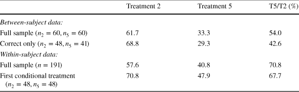
	Treatment 2	Treatment 5	T5/T2 (%)
Between-subject data:
Full sample ( $n_{2} = 60, n_{5} = 60$ )	61.7	33.3	54.0
Correct only ( $n_{2} = 48, n_{5} = 41$ )	68.8	29.3	42.6
Within-subject data:
Full sample ( $n = 191$ )	57.6	40.8	70.8
First conditional treatment ( $n_{2} = 48, n_{5} = 48$ )	70.8	47.9	67.7

7 Discussion

7.1 Relation to findings in the previous literature

Our results document that there is a lot of CC-like behavior’ in treatment 5 even though the conditioning variable is meaningless. As a reminder, the average conditional contribution in treatment 5 has a slope of approximately one quarter to one third in the conditioning variable. Also, about $30 %$ to $40 %$ of subjects in this treatment are classified as CCs. As outlined in section 1, such CC-like behavior can only be attributed to residual factors such as anchoring and confusion. In this respect, our result to some extent mirrors the findings of Ferraro and Vossler (Reference Ferraro and Vossler2010) and Burton-Chellew et al., (Reference Burton-Chellew, El Mouden and West2016). However, while the implicit message of Burton-Chellew et al., (Reference Burton-Chellew, El Mouden and West2016) is that all of CC can be accounted for by confusion and is hence an artefact of the experimental design, we find that this is not the case. Our results suggest that between one third and one half of CC is driven by inequality aversion, conformity and reciprocity.

In terms of the relative impact of the four potential drivers, our results are qualitatively similar to those of Cappelletti et al., (Reference Cappelletti, Güth and Ploner2011). Since they do not consider subject confusion in their classification, their “anchoring” accounts for what we call residual factors. Their results suggest that anchoring (residual factors) and inequality aversion are the only statistically significant drivers of CC. They estimate their relative contribution to be about the same. Although our within-subject results suggest a larger proportional role of the residual factors, our between-subject results suggest that the relative role of the two drivers might be closer to what they find. In terms of the relative impact of reciprocity and inequality aversion, our results are also in accordance with those of Ashley et al., (Reference Ashley, Ball and Eckel2010). On the other hand, our results are different from the findings of Bardsley and Sausgruber (Reference Bardsley and Sausgruber2005). They find reciprocity to have twice as large an effect as conformity, whereas we find that reciprocity has a smaller effect than conformity. As we have argued in Section 2, however, their estimate of conformity is likely to be downward-biased. We speculate that the difference to our results is driven by this bias.

It is also interesting to contrast our results with findings from field experiments on fundraising. Alpizar et al., (Reference Alpizar, Carlsson and Johansson-Stenman2008) investigate to what extent donations to a national park are driven by conformity, reciprocity and anonymity. Similarly to us, they find that conformity (to a pretended modal contribution in the past) does have an effect, albeit not a large one, whereas reciprocity (to a small gift) has a very small effect. This is in contrast to Falk (Reference Falk2007) who finds that reciprocity (to a gift) has a large effect. Whatever the effect of reciprocity to a gift might be in the field, this gift-exchange setting is different from the setting studied by us in at least three important aspects. First, it involves reciprocity between a potential donor on one side and the recipient or the fundraiser on the other side. Donors do not materially benefit from their contributions. Second, each gift is exclusively targeted toward a specific potential donor who is the only one who can reciprocate it. Third, if the gift is not followed by a (sufficiently) generous response by the potential donor, the recipient/fundraiser is left worse off. This might trigger guilt aversion and give a strong incentive to return the favor. Our setting is different. First, potential contributors are also beneficiaries of everyone’s contributions. Hence the roles of gift-givers and gift-reciprocators are not sharply defined. Second, contributions cannot be targeted toward specific individuals. Hence players might free-ride on expected reciprocity by other players. Third, there is a specific information structure. Kindness of the other group members is communicated through their higher average contribution. But, given the parameterization of the game, whenever the other group members are kinder, they are also better off even if the conditional contributor does not reciprocate. This might mitigate feelings of guilt aversion and hence reduce the incentive to return the favor. In general, this is the case whenever $(n - 1) \times MPCR > 1$ . Among FGF and its 19 replications considered by Thöni and Volk (Reference Thöni and Volk2018), this condition is satisfied in 19 studies, including FGF.Footnote ³⁶

7.2 A potential experimenter demand effect

There is a possible concern that the strong effect of residual factors in treatment 5 that we associate with confusion and anchoring is due to an an experimenter demand effect. Subjects might wonder what the experimenter expects of them since the conditioning variable is meaningless and conclude that it is an increasing conditional contribution schedule.

Our data does not allow us to identify the strength of such experimenter demand effect. However, we can rely on the results of De Quidt et al., (Reference De Quidt, Haushofer and Roth2018), who explicitly identify upper bounds on the strength of experimenter demand effects in a variety of classic elicitation tools and games used in experimental economics. We believe that the strength of the experimenter demand effect in treatment 5, if present, is bounded from above by the demand effect in what the authors refer to as a “weak demand” setting.Footnote ³⁷ They find that such effect on average moves behavior in the direction of the demand by up to 0.15 times the standard deviation of the distribution of the behavior free of the demand effect.Footnote ³⁸ In our setting, the underlying behavior is the slope of the individual subject conditional contribution schedule in treatment 5. We do not know the demand-free distribution. We approximate the standard deviation of this distribution by the standard deviation of the distribution we actually observe (0.48 in the within-subject data and 0.41 in the between-subject data). The upper bound on the demand effect implied by the findings of De Quidt et al., (Reference De Quidt, Haushofer and Roth2018) is therefore $0.15 \times 0.48 = 0.072$ in the within-subject data and $0.15 \times 0.41 = 0.062$ in the between-subject data. In either dataset, this represents only $22 %$ of our average treatment 5 slope estimate. We therefore conclude that although the experimenter demand effect might drive a part of the conditional cooperation in treatment 5, such behavior is still predominantly accounted for by anchoring and confusion.Footnote ³⁹

8 Conclusion

We use a laboratory experiment based on both within- and between-subject data to decompose CC, as identified by FGF and its replications, into parts driven by reciprocity, conformity, inequality aversion and residual factors. We associate the residual factors mostly with subject confusion and anchoring. This decomposition, including the role of the residual factors, relies on the identifying assumption of additive separability of the roles of the four drivers. Using the methodology proposed by Thöni and Volk (Reference Thöni and Volk2018), which is a slight modification of the methodology used by FGF, we find that about $30 %$ to $40 %$ of subjects are categorized as CCs even in the treatment where only residual factors play a role. This is sizeable relative to approximately $58 %$ to $70 %$ of subjects who are classified as CCs in the “baseline” treatment in which all four drivers potentially play a role and that has been considered by FGF and the follow-up literature. We obtain analogous results by estimating the slope of the average linear conditional contribution schedule as we vary the presence of the potential drivers. We find that the slope is about 0.25 to 0.32 even in the treatment where only residual factors play a role. This is sizeable relative to the slope of about 0.5 to 0.55 in the baseline treatment. That is, regardless of the experimental design (within-subject vs. between-subject) and the data analysis method (type classification vs. slope), we conclude that residual factors appear to play a major role (40% or more proportionately) in driving conditionally cooperative behavior in the lab. Regarding the role of the other three drivers, our within-subject results suggest that, of the part of conditional cooperation not accounted for by the residual factors, about 70 percent is due to inequality aversion and 30 percent due to conformity, with reciprocity playing little role.Footnote ⁴⁰

Our findings shed new light on the preference vs. noise debate following the work of Ferraro and Vossler (Reference Ferraro and Vossler2010) and Burton-Chellew et al., (Reference Burton-Chellew, El Mouden and West2016). Our results echo their findings that CC observed in the laboratory might to a large extent be driven by confusion (or anchoring). However, unlike Burton-Chellew et al.,, (Reference Burton-Chellew, El Mouden and West2016), our results indicate that there is also a sizeable preference-based portion in the CC driven mostly by inequality aversion and conformity.

Our results also have implications for research on CC for fundraising applications in the field. If taken at face value, our results imply that a positive correlation between contributions and a historical (average) contributions might to a large extent be driven by anchoring, and less so by conformity. Indeed, there are field experiments that confirm fundraising effectiveness of suitably suggested contributions that do not represent anyone’s active decisions (Charness & Cheung, Reference Charness and Cheung2013; Edwards & List, Reference Edwards and List2014). Moreover, our results imply that if contributors are shown historical contribution information, aversion to an unequal split of the contribution burden might be more important than conformity in driving contribution decisions. We do acknowledge, however, that such interpretations are only indicative since our laboratory-based results, especially those on the role of confusion, might not directly extrapolate to fundraising in the field. Rather, we hope our design will inspire similar studies in the field.

Acknowledgements

We would like to thank Michal Bauer, Simon Gächter, Wieland Müller, Simone Quercia, Rupert Sausgruber, Marie-Claire Villeval, seminar participants at RWTH Aachen University and conference participants at the 13th Nordic Conference on Behavioural and Experimental Economics, SEAM 2018, M-BEES 2019 and ESA European Meeting 2019 for useful feedback and discussion. We are also grateful to the editor and two anonymous referees for suggestions that helped to greatly improve the paper. This project was funded by the Deutsche Forschungsgemeinschaft (DFG, German Research Foundation), project no. 491485777 and Grantová Agentura České Republiky (GAČR, Czech Science Foundation), project no. 22/28064. Data, instructions and code used in this paper can be accessed at https://doi.org/10.5281/zenodo.5745354.

Funding

Open Access funding enabled and organized by Projekt DEAL.

Appendix

Kindness of a higher average contribution of the groupmates

Within the context of existing theories of intention-based reciprocity, intentions are modelled via second-order beliefs. Formally, let b be the (mean of the) second-order belief of member 1 about how much the groupmates (on average) expect him to contribute. In general, b might (and we would speculate that is likely to) depend on ${\bar{g}}_{234}$ . Therefore in what follows, we will refer to this second-order belief as $b ({\bar{g}}_{234})$ . Under such belief and conditional on ${\bar{g}}_{234}$ , member 1 expects his groupmates to expect that his payoff is $π_{1}^{e} ({\bar{g}}_{234}) \equiv 10 - 0.25 b ({\bar{g}}_{234}) + 2.25 {\bar{g}}_{234}$ . We would expect that the slope of $b (\cdot)$ is less than 9, implying that $π_{1}^{e} (\cdot)$ is strictly increasing. Hence, member 1 expects that the expectation of his payoff by the groupmates is increasing with ${\bar{g}}_{234}$ , making a higher value of ${\bar{g}}_{234}$ to be more kind. This reasoning is also borne out by using the literal definition of kindness from Rabin (Reference Rabin1993) and Dufwenberg and Kirchsteiger (Reference Dufwenberg and Kirchsteiger2004). Given whatever second-order belief b, member 1 expects that his groupmates expect his payoff to range from $10 - 0.25 b$ at the low end to $10 - 0.25 b + 22.5$ at the high end, depending on how much they contribute. Kindness of a particular value of ${\bar{g}}_{234}$ is then given by the relative location of 1’s payoff in the range of possible payoffs. This measure is given by

\begin{matrix} \frac{(10 - 0.25 b + 2.25 {\bar{g}}_{234}) - (10 - 0.25 b)}{(32.5 - 0.25 b) - (10 - 0.25 b)} = 0.1 {\bar{g}}_{234} . \end{matrix}

That is, a higher value of ${\bar{g}}_{234}$ is perceived to be kinder. Falk and Fischbacher (Reference Falk and Fischbacher2006), on the other hand, define kindness by difference in the payoff of member 1 and (adjusted to the present application) the average payoff of the groupmates given $b (\cdot)$ and ${\bar{g}}_{234}$ . This measure is given by

\begin{matrix} [10 - 0.25 b ({\bar{g}}_{234}) + 2.25 {\bar{g}}_{234}] - [10 + 0.75 b ({\bar{g}}_{234}) + 1.25 {\bar{g}}_{234}] = {\bar{g}}_{234} - b ({\bar{g}}_{234}) . \end{matrix}

According to this definition, a higher value of ${\bar{g}}_{234}$ is perceived to be kinder if and only if the slope of $b (\cdot)$ is less than 1. We would speculate that, at least for most subjects, $b (\cdot)$ is either an identity (expecting that the groupmates expect exactly matching contributions), or its slope is less than 1 (expecting that the groupmates expect some selfish bias away from exactly matching contributions). As a result, at least in a weak sense, we speculate that a higher value of ${\bar{g}}_{234}$ is perceived to be kinder under this approach as well.

Footnotes

Supplementary Information The online version contains supplementary material available at https://doi.org/10.1007/s10683-022-09756-9.

¹ A leading alternative explanation applicable to observations from laboratory studies is experimental subject confusion (Andreoni, Reference Andreoni1995; Houser & Kurzban, Reference Houser and Kurzban2002).

² See Gächter, (Reference Gächter, Frey and Stutzer2007) and Chaudhuri (Reference Chaudhuri2011) for surveys.

³ See, for example, Frey and Meier (Reference Frey and Meier2004), Alpizar et al., (Reference Alpizar, Carlsson and Johansson-Stenman2008), Croson and Shang (Reference Croson and Shang2008), Shang & Croson (Reference Shang and Croson2009), Croson et al., (Reference Croson, Handy and Shang2009) and Goeschl et al., (Reference Goeschl, Kettner, Lohse and Schwieren2018).

⁴ We speculate that imperfect game form recognition is mostly caused by insufficient attention paid to details of the environment in combination with complexity of the environment.

⁵ Along the lines of informational conformity, early contributions, or “seed money”, can affect later would-be contributors in that it signals that the goal of the fundraising campaign is worthy (List & Lucking-Reiley, Reference List and Lucking-Reiley2002; Vesterlund, Reference Vesterlund2003; Andreoni, Reference Andreoni2006). By having only one available contribution project of a known quality, our design excludes this channel. Our results therefore have implications only for normative conformity.

⁶ More specifically, this treatment eliminates direct reciprocity, but not necessarily generalized reciprocity. We discuss this point in more detail in Sects. 3 and 8.

⁷ The only case to the contrary we can think of is if a subject is indifferent across several levels of his contribution and uses anchoring on the computer-generated random conditioning variable to implement a mixed strategy.

⁸ For example, when playing against computers as in Ferraro & Vossler, (Reference Ferraro and Vossler2010) and Burton-Chellew et al., (Reference Burton-Chellew, El Mouden and West2016), a non-zero contribution that is independent of how much the three computers contribute on average suggests confusion, but not anchoring on the conditioning variable.

⁹ See the comparison of average contributions in LH and HL in their Fig. 1.

¹⁰ See their regression-based analysis summarized in Result 3 and Table 4.

¹¹ Reciprocity appears to play a somewhat more important role in their type classification analysis summarized by Result 1 and Tables 2 and 3. However, no statistical tests are provided with this analysis.

¹² As admitted by the authors themselves, their non-linear design is likely to be overly complex for subjects, as reflected in an atypically low incidence of CC relative to studies based on the linear public good game. This design also complicates the analysis of contribution data as different sub-ranges of contributions need to be analyzed separately. Consequently, the results are sensitive to which sub-range one looks at.

¹³ There is also work on whether reciprocity or inequality aversion drives punishment in public good games. Dawes et al., (Reference Dawes, Fowler, Johnson, McElreath and Smirnov2007) and Johnson et al., (Reference Johnson, Dawes, Fowler, McElreath and Smirnov2009) find that a significant part of punishment in public good games is driven by inequality aversion rather than reciprocity. On the other hand, Falk et al., (Reference Falk, Fehr and Fischbacher2005) conclude that punishment by cooperators is predominantly driven by reciprocity rather than inequality aversion.

¹⁴ There is also a related literature that addresses the same research question in the domain of a common pool resource game. Velez et al., (Reference Velez, Stranlund and Murphy2009) conduct a framed field experiment with fishermen in Colombia and find an upward-sloping best response. Based on this monotonicity, they conclude that observed behavior is best-explained by conformity.

¹⁵ We come back to the experimenter demand effect in Sect. 7.

¹⁶ The instructions and the graphical schemes were tested during three pilot sessions in order to ensure understanding by subjects.

¹⁷ We deviate from FGF in that, unlike them, we do not make subjects upfront aware that their unconditional contribution in treatment 1 might affect one’s or other group members’ payoffs in treatment 2 and other subjects’ payoffs in treatment 3. This might, under a very rigorous definition, constitute deception. We believe, however, that our design falls into the gray area of what is still an acceptable practice. When trying to define deception in economic experiments, there is a general agreement that explicitly misleading subjects is considered unacceptable (Cooper, Reference Cooper2014; Hertwig & Ortmann, Reference Hertwig and Ortmann2008; Wilson, Reference Wilson2014). This is clearly not what we do. Krawczyk (Reference Krawczyk2019) surveys experimental economists and experimental subjects in order to evaluate several potentially deceptive procedures. Our approach resembles a milder form of a procedure which he labels “linked questions,” and which ranks in the middle of the “deceptiveness” spectrum among procedures that do not explicitly mislead. Charness et al., (Reference Charness, Samek and van de Ven2020) conduct a similar survey. Our approach falls into what they label as “unexpected data use.” Among 7 potentially deceptive practices they ask about, this one is perceived to be the least deceptive.

¹⁸ Our approach is similar to the one used in a stream of literature which sorts subjects into groups based on their earlier decision without these subjects being aware of the sorting mechanism (Janssen et al., Reference Janssen, Füllbrunn and Weitzel2019; Gunnthorsdottir et al., Reference Gunnthorsdottir, Houser and McCabe2007; Wilson et al., Reference Wilson, Jaworski, Schurter and Smyth2012; Rigdon et al., Reference Rigdon, McCabe and Smith2007). The motivation for such design is likewise driven by a worry that subjects might make different earlier or later decisions if they knew about the influence of their early decision on what happens later in the experiment.

¹⁹ The kindness of this act seems intuitively obvious. To consider kindness of a higher groupmates’ average contribution within formal definitions introduced in the literature, see the Appendix.

²⁰ The usage of the terms “indirect” and “general” reciprocity is somewhat confused in the literature. We follow the terminology used by Herne et al. (Reference Herne, Lappalainen and Kestilä-Kekkonen2013). According to this terminology, direct reciprocity refers to B reciprocating to A after having been a target of an action by A. Indirect reciprocity refers to B reciprocating to A after having observed A acting toward C. Generalized reciprocity refers to B reciprocating to C after B having been a target of an action by A.

²¹ We label this belief b ( g ¯ 234 ) in the Appendix.

²² In an alternative design, the conditioning space could be expanded to include all ordered triplets of contributions. But since there are too many such triplets, this would be impractical. Alternatively, the group size could be reduced to two, making the issue go away. For comparability reasons, however, we follow the design of FGF with four group members.

²³ See Thöni & Volk, (Reference Thöni and Volk2018) for a list of references.

²⁴ There are 95 men and 96 women in the sample. We recruited men and women separately in order to achieve an approximately gender-balanced sample, but we did not insist on the particular proportion of each gender when subjects arrived to the lab.

²⁵ €1 was equal worth around CZK 25.8 and $1 was worth around CZK 22 at the time of the experiment.

²⁶ This was approximately €10.9 or $12.7 at the time of the experiment.

²⁷ For a comparison, the hourly wage that students could earn at the time of the experiment in research assistant or manual jobs typically ranged from CZK 100 to CZK 120.

²⁸ We define the proportional impact of reciprocity, conformity, inequality aversion and anchoring by β ^ R / β ^ CC , β ^ C / β ^ CC , β ^ IA / β ^ CC and β ^ RF / β ^ CC , respectively. We obtain the respective standard errors by the Delta method.

²⁹ We implement the classification using the STATA routine cctype supplied as a companion to Thöni and Volk (Reference Thöni and Volk2018).

³⁰ In the current application with a binary outcome variable, the paired sign test is equivalent to the McNemar test.

³¹ We thank an anonymous referee for suggesting this idea.

³² We are grateful to the editor and two anonymous referees for this suggestion.

³³ With this sample size, we have a power of at least 0.85 to reject the null hypothesis of a zero fraction of CCs in treatment 5 if the true fraction of CCs is 20 % . In comparison, the estimated fraction of CCs using the within-subject data for treatment 5 is 40.8 % (see Table 3). Moreover, based on the dispersion of the individual conditional contribution slopes in treatment 5 using the within-subject data, we have a power of at least 0.85 to reject the null hypothesis of a zero average slope in treatment 5 if the true slope is 0.2. In comparison, the estimated slope using the within-subject data for treatment 5 is 0.322 (see Table 2). We use equal sample sizes for treatments 2 and 5 for simplicity.

³⁴ We drew subjects from the same population and used the same laboratory as for the within-subject data. The sessions were conducted in September 2020. Almost 77% of the subjects report “Economics or Business” as their field of study. The gender ratio is almost exactly balanced with 61 men and 59 women.

³⁵ For a comparison, in treatment 1, pooling the two treatment samples, 76.7 % of subjects respond correctly to all three questions, whereas 11.7 % get one question wrong, 9.2 % get two questions wrong and 2.5 % get all three questions wrong.

³⁶ In the remaining study, ( n - 1 ) × MPCR = 1 .

³⁷ In the “weak demand” setting, subjects are given the tested hypothesis.

³⁸ The estimates presented by De Quidt et al., (Reference De Quidt, Haushofer and Roth2018) in Table 3 show the effect of the “weak demand” to be up to 0.3 times the standard deviation of the demand-free distribution of behavior. This, however, represents the difference between a positive demand and a negative demand treatment. To fit our setting, we take one half of this measure to represent the difference between a positive demand and a no demand situation.

³⁹ Moreover, in light of the standard errors of the estimated slope of the conditional contribution schedule in treatment 5 presented in Tables 2 and 4, even if the slope estimates are reduced by the upper-bound-estimates of the impact due to the demand effect, they remain highly statistically significant.

⁴⁰ In our experiment, the potential effect of reciprocity is observationally equivalent to a potential effect of guilt aversion. Likewise, it is also equivalent to a potential effect of aversion to social risk taking, or avoiding being a “sucker” (we thank an anonymous referee for pointing this interpretation to us). These confounds are not, however, important in the interpretation of the results ex post since we find relatively little effect of reciprocity. Also, the potential effect of conformity is observationally equivalent to a potential effect of generalized reciprocity. As a result, the share of CC that we attribute to conformity might also (partly) be driven by generalized reciprocity.

Springer Nature remains neutral with regard to jurisdictional claims in published maps and institutional affiliations.

References

Al-Ubaydli, Omar, & Lee, Min Sok (2012). Do you reward and punish in the way you think others expect you to?. Journal of Socio-Economics, 41(3), 336–343. 10.1016/j.socec.2012.02.002Google Scholar

Alpizar, Francisco, Carlsson, Fredrik, & Johansson-Stenman, Olof (2008). Anonymity, reciprocity, and conformity: Evidence from voluntary contributions to a national park in Costa Rica. Journal of Public Economics, 92(5), 1047–1060. 10.1016/j.jpubeco.2007.11.004CrossRef Google Scholar

Andreoni, James. (1989). Giving with impure altruism: Applications to charity and Ricardian equivalence. Journal of Political Economy,, 1447–1458.CrossRef Google Scholar

Andreoni, James (1990). Impure altruism and donations to public goods: A theory of warm-glow giving. Economic Journal, 100(401), 464–477. 10.2307/2234133CrossRef Google Scholar

Andreoni, James (1995). Cooperation in Public-Goods Experiments: Kindness or Confusion?. American Economic Review, 85(4), 891–904.Google Scholar

Andreoni, James (2006). Leadership giving in charitable fund-raising. Journal of Public Economic Theory, 8(1), 1–22. 10.1111/j.1467-9779.2006.00250.xCrossRef Google Scholar

Ashley, Richard, Ball, Sheryl, & Eckel, Catherine (2010). Motives for giving: A reanalysis of two classic public goods experiments. Southern Economic Journal, 77(1), 15–26. 10.4284/sej.2010.77.1.15CrossRef Google Scholar

Axelrod, Robert (1986). An evolutionary approach to norms. American Political Science Review, 80(4), 1095–1111. 10.2307/1960858CrossRef Google Scholar

Bardsley, Nicholas, & Sausgruber, Rupert (2005). Conformity and reciprocity in public good provision. Journal of Economic Psychology, 26(5), 664–681. 10.1016/j.joep.2005.02.001CrossRef Google Scholar

Battigalli, Pierpaolo, & Dufwenberg, Martin (2007). Guilt in Games. American Economic Review, 97(2), 170–176. 10.1257/aer.97.2.170CrossRef Google Scholar

Becker, G. S. (1974). A Theory of Social Interactions. Journal of Political Economy, 82(6), 1063–1093. 10.1086/260265CrossRef Google Scholar

Bernheim, B Douglas (1994). A theory of conformity. Journal of Political Economy, 102(5), 841–877. 10.1086/261957CrossRef Google Scholar

Bikhchandani, Sushil, Hirshleifer, David, & Welch, Ivo (1998). Learning from the behavior of others: Conformity, fads, and informational cascades. Journal of Economic Perspectives, 12(3), 151–170. 10.1257/jep.12.3.151CrossRef Google Scholar

Bolton, Gary E, & Ockenfels, Axel (2000). ERC: A theory of equity, reciprocity, and competition. American Economic Review, 90(1), 166–193. 10.1257/aer.90.1.166CrossRef Google Scholar

Burton-Chellew, Maxwell N, El Mouden, Claire, & West, Stuart A (2016). Conditional cooperation and confusion in public-goods experiments. Proceedings of the National Academy of Sciences, 113(5), 1291–1296. 10.1073/pnas.1509740113CrossRef Google Scholar PubMed

Cappelletti, Dominique., Güth, Werner, & Ploner, Matteo. (2011). Unravelling conditional cooperation. Jena Economic Research Papers, (2011–047).Google Scholar

Charness, Gary, & Dufwenberg, Martin (2006). Promises and Partnership. Econometrica, 74(6), 1579–1601. 10.1111/j.1468-0262.2006.00719.xCrossRef Google Scholar

Charness, Gary, & Cheung, Tsz (2013). A restaurant field experiment in charitable contributions. Economics Letters, 119(1), 48–49. 10.1016/j.econlet.2013.01.003CrossRef Google Scholar

Charness, Gary, Samek, Anya, & van de Ven, Jeroen. (2020). What is Considered Deception in Experimental Economics?, 2020. Version from June 29.Google Scholar

Chaudhuri, Ananish (2011). Sustaining cooperation in laboratory public goods experiments: A selective survey of the literature. Experimental Economics, 14(1), 47–83. 10.1007/s10683-010-9257-1CrossRef Google Scholar

Chou, Eileen, McConnell, Margaret, Nagel, Rosemarie, & Plott, Charles R (2009). The control of game form recognition in experiments: understanding dominant strategy failures in a simple two person “guessing” game. Experimental Economics, 12(2), 159–179. 10.1007/s10683-008-9206-4CrossRef Google Scholar

Cooper, David J (2014). A note on deception in economic experiments. Journal of Wine Economics, 9(2), 111–114. 10.1017/jwe.2014.18CrossRef Google Scholar

Croson, Rachel, & Shang, Jen (Yue) (2008). The impact of downward social information on contribution decisions. Experimental Economics, 11, 221–233. 10.1007/s10683-007-9191-zCrossRef Google Scholar

Croson, Rachel, Handy, Femida, & Shang, Jen (2009). Keeping up with the Joneses: The relationship of perceived descriptive social norms, social information, and charitable giving. Nonprofit Management and Leadership, 19(4), 467–489. 10.1002/nml.232CrossRef Google Scholar

Dawes, Christopher T, Fowler, James H, Johnson, Tim, McElreath, Richard, & Smirnov, Oleg (2007). Egalitarian motives in humans. Nature, 446(7137), 794 10.1038/nature05651CrossRef Google Scholar PubMed

Dufwenberg, Martin, & Kirchsteiger, Georg (2004). A theory of sequential reciprocity. Games and Economic Behavior, 47(2), 268–298. 10.1016/j.geb.2003.06.003CrossRef Google Scholar

Edwards, James T, & List, John A (2014). Toward an understanding of why suggestions work in charitable fundraising: Theory and evidence from a natural field experiment. Journal of Public Economics, 114, 1–13. 10.1016/j.jpubeco.2014.02.002CrossRef Google Scholar

Ellingsen, Tore, Johannesson, Magnus, Tjøtta, Sigve, & Torsvik, Gaute (2010). Testing guilt aversion. Games and Economic Behavior, 68(1), 95–107. 10.1016/j.geb.2009.04.021CrossRef Google Scholar

Engler, Yola, Kerschbamer, Rudolf, & Page, Lionel (2018). Guilt averse or reciprocal? Looking at behavioral motivations in the trust game. Journal of the Economic Science Association, 4(1), 1–14. 10.1007/s40881-018-0051-8CrossRef Google Scholar

Falk, Armin (2007). Gift exchange in the field. Econometrica, 75(5), 1501–1511. 10.1111/j.1468-0262.2007.00800.xCrossRef Google Scholar

Falk, Armin, & Fischbacher, Urs (2006). A theory of reciprocity. Games and Economic Behavior, 54(2), 293–315. 10.1016/j.geb.2005.03.001CrossRef Google Scholar

Falk, Armin, Fehr, Ernst, & Fischbacher, Urs (2005). Driving forces behind informal sanctions. Econometrica, 73(6), 2017–2030. 10.1111/j.1468-0262.2005.00644.xCrossRef Google Scholar

Fehr, Ernst, & Schmidt, Klaus M (1999). A theory of fairness, competition, and cooperation. Quarterly Journal of Economics, 114(3), 817–868. 10.1162/003355399556151CrossRef Google Scholar

Fehr, Ernst, & Fischbacher, Urs (2004). Social norms and human cooperation. Trends in Cognitive Sciences, 8(4), 185–190. 10.1016/j.tics.2004.02.007CrossRef Google Scholar PubMed

Ferraro, Paul J., & Vossler, Christian A. (2010). The Source and Significance of Confusion in Public Goods Experiments. B.E. Journal of Economic Analysis & Policy, 10, (1).CrossRef Google Scholar

Fischbacher, Urs (2007). z-Tree: Zurich toolbox for ready-made economic experiments. Experimental Economics, 10(2), 171–178. 10.1007/s10683-006-9159-4CrossRef Google Scholar

Fischbacher, Urs, Gächter, Simon, & Fehr, Ernst (2001). Are People Conditionally Cooperative ? Evidence from a Public Goods Experiment. Economics Letters, 71(3), 397–404. 10.1016/S0165-1765(01)00394-9CrossRef Google Scholar

Frey, Bruno S, & Meier, Stephan (2004). Social Comparisons and Pro-social Behavior: Testing “Conditional Cooperation” in a Field Experiment. American Economic Review, 94(5), 1717–1722. 10.1257/0002828043052187CrossRef Google Scholar

Gächter, Simon Frey, Bruno S, & Stutzer, Alois (2007). Conditional cooperation: Behavioral regularities from the lab and the field and their policy implications. Economics and Psychology. A Promising New Cross-Disciplinary Field, Cambridge: MIT Press 19–50.CrossRef Google Scholar

Goeschl, Timo, & Lohse, Johannes (2018). Cooperation in public good games. Calculated or confused?. European Economic Review, 107, 185–203. 10.1016/j.euroecorev.2018.05.007CrossRef Google Scholar

Goeschl, Timo, Kettner, Sara Elisa, Lohse, Johannes, & Schwieren, Christiane. (2018). From Social Information to Social Norms: Evidence from Two Experiments on Donation Behaviour. Games, 9, (4).CrossRef Google Scholar

Greiner, Ben (2015). Subject pool recruitment procedures: organizing experiments with ORSEE. Journal of the Economic Science Association, 1(1), 114–125. 10.1007/s40881-015-0004-4CrossRef Google Scholar

Gul, Faruk, & Pesendorfer, Wolfgang (2016). Interdependent preference models as a theory of intentions. Journal of Economic Theory, 165, 179–208. 10.1016/j.jet.2016.04.009CrossRef Google Scholar

Gunnthorsdottir, Anna, Houser, Daniel, & McCabe, Kevin (2007). Disposition, history and contributions in public goods experiments. Journal of Economic Behavior & Organization, 62(2), 304–315. 10.1016/j.jebo.2005.03.008CrossRef Google Scholar

Herne, Kaisa, Lappalainen, Olli, & Kestilä-Kekkonen, Elina (2013). Experimental comparison of direct, general, and indirect reciprocity. Journal of Socio-Economics, 45, 38–46. 10.1016/j.socec.2013.04.003Google Scholar

Hertwig, Ralph, & Ortmann, Andreas (2008). Deception in experiments: Revisiting the arguments in its defense. Ethics & behavior, 18(1), 59–92. 10.1080/10508420701712990CrossRef Google Scholar

Houser, Daniel, & Kurzban, Robert (2002). Revisiting Kindness and Confusion in Public Goods Experiments. American Economic Review, 92(4), 1062–1069. 10.1257/00028280260344605CrossRef Google Scholar

Janssen, Dirk-Jan, Füllbrunn, Sascha, & Weitzel, Utz (2019). Individual speculative behavior and overpricing in experimental asset markets. Experimental Economics, 22(3), 653–675. 10.1007/s10683-018-9565-4CrossRef Google Scholar

Johnson, Tim, Dawes, Christopher T, Fowler, James H, McElreath, Richard, & Smirnov, Oleg (2009). The role of egalitarian motives in altruistic punishment. Economics Letters, 102(3), 192–194. 10.1016/j.econlet.2009.01.003CrossRef Google Scholar

Keser, Claudia (1996). Voluntary contributions to a public good when partial contribution is a dominant strategy. Economics Letters, 50(3), 359–366. 10.1016/0165-1765(95)00769-5CrossRef Google Scholar

Krawczyk, Michał (2019). What should be regarded as deception in experimental economics? Evidence from a survey of researchers and subjects. Journal of Behavioral and Experimental Economics, 79, 110–118. 10.1016/j.socec.2019.01.008CrossRef Google Scholar

Laffont, Jean-Jacques (1975). Macroeconomic constraints, economic efficiency and ethics: An introduction to Kantian economics. Economica, 42(168), 430–437. 10.2307/2553800CrossRef Google Scholar

Ledyard, John Kagel, John, & Roth, Alvin (1995). Public goods: A survey of experimental research. Handbook of Experimental Economics, USA: Princeton University Press.Google Scholar

Levine, David K (1998). Modeling Altruism and Spitefulness in Experiments. Review of Economic Dynamics, 1(3), 593–622. 10.1006/redy.1998.0023CrossRef Google Scholar

List, John A, & Lucking-Reiley, David (2002). The Effects of Seed Money and Refunds on Charitable Giving: Experimental Evidence from a University Capital Campaign. Journal of Political Economy, 110(1), 215–233. 10.1086/324392CrossRef Google Scholar

De Quidt, Jonathan, Haushofer, Johannes, & Roth, Christopher (2018). Measuring and bounding experimenter demand. American Economic Review, 108(11), 3266–3302. 10.1257/aer.20171330CrossRef Google Scholar

Rabin, Matthew. (1993). Incorporating fairness into game theory and economics. American Economic Review,, 1281–1302.Google Scholar

Recalde, María P, Riedl, Arno, & Vesterlund, Lise (2018). Error-prone inference from response time: The case of intuitive generosity in public-good games. Journal of Public Economics, 160, 132–147. 10.1016/j.jpubeco.2018.02.010CrossRef Google Scholar

Rigdon, Mary L, McCabe, Kevin A, & Smith, Vernon L (2007). Sustaining cooperation in trust games. The Economic Journal, 117(522), 991–1007. 10.1111/j.1468-0297.2007.02075.xCrossRef Google Scholar

Rotemberg, Julio J (2008). Minimally acceptable altruism and the ultimatum game. Journal of Economic Behavior & Organization, 66(3), 457–476. 10.1016/j.jebo.2006.06.008CrossRef Google Scholar

Shang, Jen, & Croson, Rachel (2009). A Field Experiment in Charitable Contribution: The Impact of Social Information on the Voluntary Provision of Public Goods. The Economic Journal, 119(540), 1422–1439. 10.1111/j.1468-0297.2009.02267.xCrossRef Google Scholar

Thöni, Christian, & Volk, Stefan (2018). Conditional cooperation: Review and refinement. Economics Letters, 171, 37–40. 10.1016/j.econlet.2018.06.022CrossRef Google Scholar

Tversky, Amos, & Kahneman, Daniel (1974). Judgment under uncertainty: Heuristics and biases. Science, 185(4157), 1124–1131. 10.1126/science.185.4157.1124CrossRef Google Scholar PubMed

Velez, Maria Alejandra, Stranlund, John K, & Murphy, James J (2009). What motivates common pool resource users? Experimental evidence from the field. Journal of Economic Behavior & Organization, 70(3), 485–497. 10.1016/j.jebo.2008.02.008CrossRef Google Scholar

Vesterlund, Lise (2003). The informational value of sequential fundraising. Journal of Public Economics, 87(3–4), 627–657. 10.1016/S0047-2727(01)00187-6CrossRef Google Scholar

Wilson, Bart J (2014). The meaning of deceive in experimental economic science, In The Oxford Handbook of Professional Economic Ethics: Oxford University Press, New York, NY.Google Scholar

Wilson, Bart J, Jaworski, Taylor, Schurter, Karl E, & Smyth, Andrew (2012). The ecological and civil mainsprings of property: An experimental economic history of whalers’ rules of capture. The Journal of Law, Economics, and Organization, 28(4), 617–656. 10.1093/jleo/ewr024CrossRef Google Scholar

Table 1 Presence of behavior drivers in the four treatments

Fig. 1 Histogram of unconditional contributions

Fig. 2 Average conditional contribution by value of the conditioning variable and treatment

Table 2 Estimated slope of the average conditional contribution schedule and its decomposition

Table 3 Conditional contributor type classification by treatment (% of all subjects, shares of conditional cooperators in bolded)

Fig. 3 Average conditional contribution by value of the conditioning variable and treatment

Fig. 4 Average conditional contribution by value of the conditioning variable, treatment and quiz response record

Table 4 Estimated slope of the average conditional contribution schedule

Table 5 Conditional contributor type classification by treatment (% of all subjects)

Katuščák and Miklánek supplementary material

File 4.3 MB

Article contents

What drives conditional cooperation in public good games?

Abstract

Keywords

JEL classification

1 Introduction

2 Related literature

2.1 Reciprocity, conformity, inequality aversion and anchoring

2.2 Confusion

3 Experimental design and identification strategy

3.1 Procedure

3.2 Treatments

3.3 Identification strategy

3.4 Logistics

4 Methodology for data analysis

4.1 Slope decomposition

4.2 Subject type classification

5 Results

5.1 Preliminary analysis

5.2 Slope decomposition

5.3 Subject type classification

5.4 Conditioning on conditional cooperators

6 Robustness in a between-subject design

6.1 Design modifications

6.2 Results

7 Discussion

7.1 Relation to findings in the previous literature

7.2 A potential experimenter demand effect

8 Conclusion

Acknowledgements

Funding

Appendix

Kindness of a higher average contribution of the groupmates

Footnotes

References

Katuščák and Miklánek supplementary material

Save article to Kindle

Save article to Dropbox

Save article to Google Drive

Reply to: Submit a response

Your details

You have entered the maximum number of contributors

Conflicting interests