


1 Introduction
Coordination failures are some of the most important sources of economic inefficiencies. Coordination games have been used extensively to study both theoretically and experimentally the sources and remedies of coordination failures. As observed by Crawford et al. (Reference Crawford, Gneezy and Rottenstreich2008), one instance where severe coordination failures take place is when coordination entails asymmetric payoffs for the players involved. In this paper, we consider a class of 2 × 2 coordination games with highly asymmetric payoffs between the players, and examine through laboratory experiments if ex post voluntary transfer of payoffs helps eliminate coordination failures and increase efficient coordination.
Formally, an inequality game is a 2 × 2 coordination game with two Nash equilibria (NE) (X, X) and (Y, Y). Player 1 earns a strictly higher payoff than player 2 at every action profile except at (Y, Y), where they earn the same payoff. However, the sum of payoffs at (Y, Y) is substantially lower than that at (X, X), implying a tension between efficiency and equity. The inequality games are further classified into ComMon-interest (CM) inequality games in which both players’ payoffs are higher at (X, X) than at (Y, Y), and ConFlicting-interest (CF) inequality games in which player 1’s payoff is higher but player 2’s payoff is lower, at (X, X) than at (Y, Y). Examples of CM and CF inequality games are presented in Table 1. The inequality games are also parametrized by the degree of inequality between the two players’ payoffs.
Table 1 Inequality games
|
CM |
CF |
||||||||
|---|---|---|---|---|---|---|---|---|---|
|
X |
Y |
X |
Y |
||||||
|
X |
440, |
110 |
60, |
50 |
X |
320, |
80 |
60, |
20 |
|
Y |
380, |
60 |
100, |
100 |
Y |
260, |
60 |
100, |
100 |
(X, X) efficient coordination; (Y, Y) equitable coordination
The redistribution scheme we propose allows both players to voluntarily transfer their payoffs to the other player after the play of the inequality game. Although such a scheme will have no impact on the outcome of the game under self-interested preferences, our main objective is to analyze its functioning in a laboratory where subjects’ motivation may come from other sources than self-interest.
The efficiency-equity trade-off between the two NE in the inequality games can be a fundamental source of coordination failures. The players playing CM and CF games also can have sufficiently different motivations when choosing their actions. In CM games, coordination on the Pareto efficient profile (X, X) will result unless the players are, or expect the other player to be, sufficiently inequality averse. In CF games, on the other hand, coordination on (X, X) would be more difficult since it entails a material sacrifice by player 2 compared with coordination on (Y, Y). With ex post redistribution, this difference in the motivations between the CM and CF games can have a significant impact on the final outcome. In other words, when (X, X) is realized in the CM games, player 1 may interpret it as a result of player 2’s self-interested behavior, and may find little reason to reciprocate 2’s choice of X with payoff transfer to him. On the other hand, if (X, X) is realized in CF games, player 1 may interpret it as resulting from 2’s self-sacrifice to achieve an outcome which benefits 1. Player 1 may hence have incentive to reciprocate this with payoff transfer. Expecting this, however, player 2 may strategically choose X in CF to his own benefit.
In our experiments, each subject is randomly assigned the role of either player 1 or player 2, and is randomly and anonymously matched with a subject who is assigned the other role. The experiment consists of three parts with the subject role fixed throughout. In the first part, we have a half of the subjects in each role make a dictator decision over the action profiles of each inequality game. In the second part, the subjects play a series of inequality games in a standard way. In the third part, they play the inequality games under the redistribution scheme. Our design choice to have the same set of subjects play the games with no redistribution first and then with redistribution next, and provide in the instructions detailed information on how the payoffs are determined by the actions, is motivated by the importance of having the subjects understand the externalities involved in their decision making in the inequality games and the consequences of possible coordination failures. The within-subject design also allows us to associate the heterogeneity in the subjects’ behavior with their preferences and beliefs about the behavior of the other player.
Our results show that the redistribution scheme induces significantly positive transfer by player 1 in both CM and CF games. Positive transfer takes place almost exclusively when player 2 chooses action X which corresponds to the efficient NE preferred by player 1. The size and frequency of transfer is higher in CF games than in CM games, and increasing inequality increases the size of transfer but not the frequency of positive transfer. Comparison of the results with and without the redistribution scheme shows that the scheme induces the efficient NE (X, X) strongly significantly in CF games, but only weakly in CM games. We also find that the scheme increases the sum of the two players’ payoffs significantly in CF games but only insignificantly in CM games, and significantly improves equity as measured by the payoff ratio between the two players in both CF and CM games.
Since the introduction of ex post payoff redistribution has no impact on the behavior of self-interested individuals, the observed increase in efficient coordination and positive transfer imply the presence of distributive social preferences and/or reciprocity. We attempt to identify the source of these effects based on some key observations. In particular, we remark that positive transfer by player 1 to player 2 takes place almost exclusively following 2’s choice of X. This suggests that player 1 reciprocates player 2’s action choice that benefits player 1. Furthermore, the observed difference between CM and CF games suggests that player 1 perceives the level of kindness entailed in 2’s choice of X differently in the two games. Specifically, the choice of X by player 2 can result from self-interest in CM, but entails a sacrifice in CF. We suppose that player 1’s reciprocity is strengthened by the presence of self-sacrifice by player 2, and postulate a psychological utility function that explicitly accounts for sacrifice. Taking advantage of the within-subject design, we also attempt to identify the subjects’ motivations by examining their behavior in different tasks. In particular, we find that the increased choice of action X by the role 2 subjects in the redistribution scheme is likely motivated by self-interest: They choose X in anticipation of the choice of X and positive transfer by role 1.
The key contributions of the present paper are summarized as follows. First, we show that social preferences can have a significant impact on the play of coordination games. The literature on social preferences has largely ignored coordination games perhaps because of the intuitive perception that social preferences will only contribute to an increase in coordination. We present a formal framework to test this intuition and identify the working of social preferences in the presence of a tension between equality and efficiency. Second and relatedly, we identify self-sacrifice as a critical trigger of positive reciprocity. Third, we find that individuals respond differently to increase in inequality, and that the increase in efficient coordination in the presence of redistribution opportunities is brought about by those who are intrinsically concerned about inequality and/or the own payoffs. Finally, our methodological contribution lies in the formulation of a class of coordination games with payoff asymmetry between the two players. Specifically, this class usefully nests both common and conflicting interests games with varying degrees of inequality and allows us to study the effects of these elements while controlling for the confounding effect of risk dominance.
The paper is organized as follows. The next section discusses the related literature. The inequality game and the redistribution scheme are described in Sect. 3, and testable implications of social preferences are presented in Sect. 4. Section 5 describes the experimental design, and Sect. 6 presents the analysis. The heterogeneous motives behind the observed action choices and transfer decisions are discussed in Sect. 7. We conclude with a discussion in Sect. 8.
2 Related literature
Reciprocity-based mechanisms originate in the literature on public good games. Reciprocity in the form of a punishment or disapproval of other players is the focus of early study by Fehr and Gächter (Reference Fehr and Gächter2000) and Masclet et al. (Reference Masclet, Noussair, Tucker and Villeval2003).Footnote 1 While reciprocity is at the core of our analysis, asymmetry between the players in our model offers a significantly different perspective from that in the symmetric environment in the early literature.
The public good literature also offers extensive research on the possible distortion of behavior associated with inequality among the players: Asymmetry is introduced either in the level of individual return (MPCR - marginal per capita return), or in the level of initial endowment (income) of each individual. The findings are largely inconclusive.Footnote 2 Combining asymmetry with redistribution in public good games, Dekel et al. (Reference Dekel, Fischer and Zultan2017) and Gangadharan et al. (Reference Gangadharan, Nikiforakis and Villeval2017) present analysis most closely related to the present paper. When players with positive and negative MPCR’s interact, and redistribution takes the form of either a punishment or reward, Dekel et al. (Reference Dekel, Fischer and Zultan2017) observe that communication coupled with a reward increases contribution substantially. When players may ex post reward the others, Gangadharan et al. (Reference Gangadharan, Nikiforakis and Villeval2017) also find a positive impact of communication on both earnings and contribution, but show that its impact is significantly weakened in the presence of heterogeneity in MPCR.Footnote 3 While the present model shares many features with the papers on public good games with heterogeneity and ex post redistribution, its use of coordination games highlights the role of reciprocity more clearly. Specifically, it is intuitive that player 2’s choice of X corresponding to the efficient coordination is a favor given to player 1, and that payoff transfer from 1 to 2 is a direct way of returning the favor.Footnote 4, Footnote 5
Positive reciprocity is studied most intensively in the trust games. Although several authors have studied the interplay of inequality and reciprocity in the trust games, our framework is different in some critical dimensions.Footnote 6 First, the sequential nature of a trust game presents no coordination issue which is the source of strategic uncertainty and a central focus of our study. Second, while a sender’s action of trust in a trust game is a clear message requesting reciprocation, the simultaneous action choices in an inequality game are strategic and hence much less straightforward to interpret. Third, players in a trust game have inherently asymmetric roles as a sender and receiver, whereas the players of an inequality game are symmetric except for their payoffs. Fourth, the trust games do not allow us to study the effect of self-sacrifice as is done here.
Turning to the extensive literature on coordination games experiments, the primary focus is on the comparison between payoff dominance and risk dominance as the effective predictor of the outcome of play.Footnote 7 The literature on coordination games also investigates ways to eliminate coordination failures, and finds mixed evidence on the effectiveness of forward induction and correlated equilibrium recommendations.Footnote 8 Importantly, our analysis controls for the effect of risk-dominance by using games that have a constant level of risk dominance. Furthermore, while forward induction or correlated equilibrium recommendations are based on self-regarding preferences, the working of the redistribution mechanism hinges on social preferences.
3 Models of inequality and redistribution
3.1 Inequality games
Formally, an inequality game G is a 2 × 2 coordination game: Each player i chooses his action
 from the set
 , and their payoff functions are given by
For the interpretation of these payoff functions, suppose that each player i chooses whether to allocate his resource to either their private activity (
 ) or an activity toward a public project (
 ). The private activity generates positive externalities to the other player, whereas the public project results in a success if and only if both players allocate their resources to it. The successful public project is worth a to each player, whereas player i’s private activity is worth b to himself and worth
 to the other player j. When both players engage in private activities, the utility of each player is simply the sum of the benefits from his and the other player’s activities.Footnote 9 We suppose that the externality benefit that 2’s private activity creates for 1 is larger than the externality benefit that 1’s private activity creates for 2:

Note that the second condition is the only source of inequality between the two players. Writing X for
 , and Y for
 , we can depict the payoff table as in Table 2.Footnote 10
Table 2 Inequality game:

|
P1
|
X |
Y |
||
|---|---|---|---|---|
|
X |
|
|
b |
|
|
Y |
|
b |
a |
a |


Since
 , both (X, X) and (Y, Y) are pure NE. We also assume (i)

 (X, X) uniquely maximizes the sum of payoffs, (ii)


 for
for
 , and (iii)

 (X, X) is risk dominant. It follows from (ii) that (Y, Y) is the only profile in which the two players earn the same payoff. We further focus on the following subclasses of inequality games: An inequality game has ComMon-interest (CM) if
 , and has ConFlicting-interest (CF) if
 . In other words, if an inequality game has CM, then both players 1 and 2 prefer the NE (X, X) to the NE (Y, Y) (in terms of material payoffs), whereas if it has CF, then player 1 prefers (X, X) to (Y, Y) and player 2 prefers (Y, Y) to (X, X).
In our experiments, we set
 and
and
 and choose six combinations of
 and
and
 as in Table 3. This results in three CM inequality games denoted CM2, CM4 and CM6, and three CF inequality games denoted CF2, CF4 and CF6. The suffix represents the degree of inequality between the players and is equal to the payoff ratio at (X, X):
Since
 , within each class of games, the larger is k, the larger is the payoff difference at (X, X).Footnote 11 The resulting payoff tables are depicted in Tables 4 and 5. Note that all CM games are the same in terms of player 2’s payoffs, and so are all CF games. Furthermore, since a and b are held constant in all games, so is the risk dominance level of (X, X).
Table 3 Parameter specifications
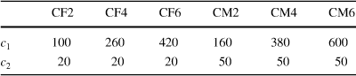
|
CF2 |
CF4 |
CF6 |
CM2 |
CM4 |
CM6 |
|
|---|---|---|---|---|---|---|
|
|
100 |
260 |
420 |
160 |
380 |
600 |
|
|
20 |
20 |
20 |
50 |
50 |
50 |


Table 4 CM inequality games
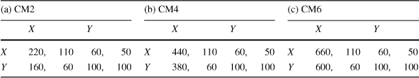
|
(a) CM2 |
(b) CM4 |
(c) CM6 |
||||||||||||
|---|---|---|---|---|---|---|---|---|---|---|---|---|---|---|
|
X |
Y |
X |
Y |
X |
Y |
|||||||||
|
X |
220, |
110 |
60, |
50 |
X |
440, |
110 |
60, |
50 |
X |
660, |
110 |
60, |
50 |
|
Y |
160, |
60 |
100, |
100 |
Y |
380, |
60 |
100, |
100 |
Y |
600, |
60 |
100, |
100 |
Table 5 CF inequality games
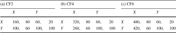
|
(a) CF2 |
(b) CF4 |
(c) CF6 |
||||||||||||
|---|---|---|---|---|---|---|---|---|---|---|---|---|---|---|
|
X |
Y |
X |
Y |
X |
Y |
|||||||||
|
X |
160, |
80 |
60, |
20 |
X |
320, |
80 |
60, |
20 |
X |
480, |
80 |
60, |
20 |
|
Y |
100, |
60 |
100, |
100 |
Y |
260, |
60 |
100, |
100 |
Y |
420, |
60 |
100, |
100 |
3.2 Voluntary redistribution
Let
 denote player i’s final material payoff after the possible redistribution of their payoffs. Task 1 (T1) is the baseline scheme in which no redistribution takes place after the play of the inequality game G. In T1, the players’ final payoffs equal their payoffs from G:
 . Task 2 (T2), on the other hand, is the redistribution scheme in which the players may give part or all of their payoffs to the other player after publicly observing the outcome of the inequality game. If player i gives
 payoff points to player j (
 ), then i’s final (material) payoff is given by (
 )
)

Task 0 (T0) is the dictator scheme in which the final allocation is determined by only one of the players. Specifically, one player in each pair makes a choice among four payoff pairs that correspond to the four cells of the payoff table.
4 Equilibrium under reciprocity
Player i’s strategy
 in T0 is the choice of an action profile, whereas his strategy in T1 is
 . Player i’s strategy in T2 is a pair
 , where
 is the action choice and
 is the transfer function that determines transfer to the other player j for each realization of the action profile. The subgame perfect equilibrium (SPE)
 is defined in the standard manner.
The players have self-interest preferences if their utilities equal their material payoffs (2):
 for
for
 , 2. Under self-interest preferences, no redistribution takes place in any SPE of T2 (i.e.,
 for
for
 , 2), and x is consistent with an SPE of T2 if and only if it is a NE of G.
We say that the players have reciprocity preferences if they reward the other player through positive transfer for the favor given to them in the play of the inequality game. Specifically, we suppose that the reciprocity preferences are given by

where for
 (
(
 , 2),
, 2),

The second term of
 represents player i’s reciprocity concerns, and
 is the reciprocity weight that measures how kind j is toward i through his action choice in G. Specifically, player i takes
 as the reference point, and considers j to be kind when j’s alternative action choice
 raises i’s payoff above a. That is, player i places a strictly positive weight
 on j’s material payoff if and only if
 .Footnote 12 If j’s choice of X not only raises i’s payoff above a but also lowers j’s own payoff from a, then i regards it as the sacrifice made by j in raising i’s payoff, and rewards j even more strongly by placing a higher weight on j’s material payoff. In the CM inequality games, for example,
 and
and
 since both players are better off at (X, X) than at (Y, Y). On the other hand, in the CF inequality games,
 and
and
 since player 1 is better off and player 2 is worse off at (X, X) than at (Y, Y).Footnote 13 The following proposition holds for the SPE of T2 under reciprocal preferences.
Proposition 1
(SPE transfer under reciprocity) Suppose that the players’ preferences are given by (3).
 is an SPE transfer in T2 if and only if for
 ,
,
 , 2,
, 2,
 ,
,

The SPE transfer
 in (4) is illustrated in Fig. 1. In what follows, we restrict attention to the case where the reciprocity weights
 are not too large so that neither player transfers his entire payoff
 .Footnote 14 When the parameters are in such a range, Fig. 1 shows that at most one player makes a positive transfer, and which player does so depends on the relative magnitude of the reciprocity weights. In particular, as long as those weights are similar in size, it is player 1 who makes positive transfer given that his payoff
 is much larger than 2’s payoff
 . Our hypotheses under the reciprocity preferences (3) are as follows.Footnote 15
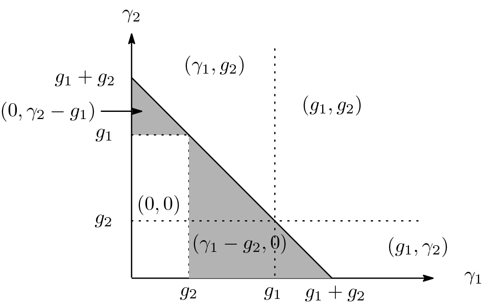
Fig. 1 SPE transfer
 as a function of the reciprocity weights

Hypothesis 1
Under the reciprocity preferences (3),
a. (X, X) is played more often in T2 than in T1.
b. Player 1 makes positive transfer only if player 2 has chosen X, and is more likely to make positive transfer at (X, X) in CF than in CM.
c. The action choice as well as transfer at (X, X) are both unaffected by the degree k of inequality.
Hypotheses Footnote 1a and Footnote 1b are our main hypotheses. The reciprocity preferences as defined in (3) generate behavior different from self-interest only in T2, and no difference is expected either in T0 or T1. As competing hypotheses, we consider the distributional social preferences as follows. The players have inefficiency aversion (IEA) preferences if they are concerned about the efficiency of an outcome as measured by the sum of their material payoffs. Specifically, we suppose that

where
 represents the degree of the inefficiency concerns relative to the own material payoff. The players have inequality aversion (IQA) preferences if they dislike inequality in their material payoffs. Specifically, we suppose that

where
 represents the degree of the inequality concerns relative to the own material payoff.Footnote 16 The implications of these preferences are as follows.Footnote 17
Hypothesis 2
Under the IEA preferences (5),
a. The action profiles are the same under T1 and T2.
b. No transfer takes place in T2.
c. (X, X) is played more often as the degree k of inequality increases.
Hypothesis 3
Under the IQA preferences (6),Footnote 18
a. (X, X) is played more often in T2 than in T1.
b. Player 1 makes positive transfer except at (Y, Y).
c. As the degree k of inequality increases, (Y, Y) is played more often in T1. The size of transfer in T2 is larger when k is larger, or in CM than in CF.
5 Experimental design
The experiments were conducted at the Experimental Economics Laboratory at the ISER, Osaka University, with the subjects recruited from undergraduate and graduate students of Osaka University of various majors. There were six sessions with a total of 124 subjects (four sessions of 20 subjects and two sessions of 22 subjects). No subject attended more than one session. The subjects in each session were divided randomly into two groups of the same size with the first group of subjects assigned the role of player 1, and the second group assigned the role of player 2. The player roles stay the same throughout the session. The role assignment is done privately on the PC screen in front of each subject. The instruction presents the payoff formula (1), and provides its illustration by means of numerical examples and graphs.Footnote 19, Footnote 20 The inclusion of the payoff formula is intended to help the subjects understand the source of inequality between the two roles, and also the externalities involved in their decision making. The payoff matrix is shown also on the PC screen in front of each subject. At the end of each session, the earning of a subject is computed from the sum of his/her payoff points during the session with the conversion rate of 1 payoff point to JPY1.3.Footnote 21 The average earnings are JPY9946.1 for the role 1 subjects and JPY3122.8 for the role 2 subjects.Footnote 22 The subjects were also given a record sheet in which they describe their action and transfer choices as well as the reason behind those choices.
The experiments adopt the within-subject design and every session is divided into three task blocks that correspond to T0–T2 described in the previous section. Each task block in turn consists of six rounds that correspond to the six inequality games CF2-CF6 and CM2-CM6. In all four sessions, the ordering of the task blocks is fixed and given by

As mentioned in the Introduction, the fixed task order was adopted so that the subjects would become fully aware of the externalities involved in their decision making through the standard play of the inequality games in T1.Footnote 23 The six games appear in random order in the six rounds of each task block. In T0, a half of the role 1 subjects and a half of the role 2 subjects are randomly chosen to make a choice.Footnote 24 After every round, each subject observes his and the other player’s action choices on their PC screen, and then is anonymously rematched to another subject of the opposite role in the stranger format. Since ten or eleven pairs are formed in each session consisting of 18 rounds, the probability that the same pair of subjects are matched is positive. One concern may be that it generates stronger incentive to coordinate on the efficient action profile than in the one-shot environment. The literature on repeated prisoners’ dilemma however finds that cooperation rates are not high under random matching (Duffy and Ochs Reference Duffy and Ochs2009). Furthermore, since the same format is used for T1 and T2, the marginal impact of such an incentive on the effectiveness of T2, if any, would be smaller.Footnote 25
6 Analysis
6.1 Dictator decisions
Fig. 2 Outcome distribution in T0
We begin by examining the outcome of the dictator decision task (T0). Figure 2 shows the frequency of each of four choices for CM and CF games, where
 ,
,
 ,
,
 , and
, and
 . As seen, the subjects’ choices are almost entirely limited to (X, X) and (Y, Y), which are NE of the game.Footnote 26 Additionally, the role 1 subjects choose (X, X) more than 94% of the time, whereas the choice of the role 2 subjects is approximately reversed depending on whether the game is CM or CF. In CM, they choose (X, X) more than 90% of the time, whereas in most cases of CF, they choose (Y, Y) 80% of the time.Footnote 27 The inequality dummy k is mostly insignificant in both CM and CF.Footnote 28
Role 1’s choice of (X, X) is consistent with self-interest and IEA, whereas role 2’s choice of (X, X) in CM and (Y, Y) in CF is consistent with self-interest and IQA.
Observation 1
(Dictator decision) The behavior of the role 1 subjects in T0 is mostly consistent with self-interest and IEA. The behavior of the role 2 subjects in T0 is mostly consistent with self-interest and IQA. Footnote 29
6.2 Action choice
Figure 3 shows the frequency of each action (X and Y) by each subject role. As seen, there is a significant difference in the subjects’ action choice in T1 and T2, and the difference is more prominent in CF: Going from CM-T1 to CM-T2, the choice of X increases by 6 percentage points for role 1 (90%
 96%) and by 4 percentage points for role 2 (90%
 94%). On the other hand, going from CF-T1 to CF-T2, the choice of X increases by 16 percentage points for role 1 (68%
 84%), and 10 percentage points for role 2 (73%
 83%). It also shows that both roles choose Y more often in CF than in CM. These observations are confirmed by the random effects logit regressions in Table 11 in Appendix A.1, where the dependent variable equals one if a subject chooses Y. Models (4) and (6) in Table 11, which include inequality dummies k
 and k
and k
 , show that increasing inequality has different effects in CM and CF: While higher inequality overall has a positive impact on the choice of Y in CM, higher inequality has little to no impact in CF. In CM where the increasing inequality increases the choice of Y, this effect is independent of the subject role (model (5)). The subject role has no significant impact on the action choice in CM and CF (models (2) and (3)). This is in sharp contrast with our observation in CF-T0, where the dominant choice is
 for role 1 and
 for role 2.Footnote 30 The observation on the action choice can be summarized as follows:
Fig. 3 Action choices in T1 and T2. ** and ***: significant difference at 5% and 1%, respectively, between the respective pair of distributions (
 ). Shown in each column are the numbers of each action choice aggregated for k = 2, 4, and 6
Observation 2
(Action choice)
1. In CF, T2 raises the choice of X compared with T1.
2. Higher inequality increases the choice of Y in CM.
Observation Footnote 2.1 supports our main reciprocity Hypothesis Footnote 1a as well as the IQA Hypothesis Footnote 3a but not the IEA Hypothesis Footnote 2a. The effect of inequality in Observation Footnote 2.2 on CM is also consistent with the IQA Hypothesis Footnote 3c, but not with the IEA Hypothesis Footnote 1c or the reciprocity Hypothesis Footnote 2c.
6.3 Coordination
Table 6 Realization of action profiles
|
Action profile |
CM |
CF |
||||||
|---|---|---|---|---|---|---|---|---|
|
T0 |
T1 |
T2 |
T0 |
T1 |
T2 |
|||
|
Role 1 |
Role 2 |
Role 1 |
Role 2 |
|||||
|
(X, X) |
94 |
83 |
151 |
167 |
93 |
16 |
89 |
130 |
|
(Y, Y) |
2 |
6 |
2 |
0 |
2 |
73 |
14 |
5 |
|
(X, Y) |
0 |
1 |
17 |
12 |
1 |
0 |
37 |
26 |
|
(Y, X) |
0 |
0 |
16 |
7 |
0 |
1 |
46 |
25 |
|
p-value (
|
||||||||
|
T0=T1=T2 |
0.00 |
0.00 |
0.00 |
0.00 |
||||
|
T1=T2 |
0.07 |
0.00 |
||||||
|
CM=CF |
0.00 |
0.00 |
0.00 |
|||||

The three lines in the bottom report the p-values of the
 tests of the hypothesis that the distributions are the same for T0-T2 (first line), between T1 and T2 (second line), and between CM and CF (third line)
Table 6 describes the realized distribution of four action profiles in T0 through T2. It shows that the redistribution scheme induces efficient coordination particularly effectively in CF: Going from T1 to T2, the efficient coordination (X, X) increases by 9% percentage points (81%
 90%) in CM, but by 22 percentage points in CF (48%
 70%). Furthermore, the redistribution scheme also reduces coordination failures much more substantially in CF: Coordination failures (X, Y) and (Y, X) decrease by 8 percentage points in CM (18%
 10%), whereas they decrease by 18% percentage points in CF (45%
 27%). In fact, the difference in the distributions between T1 and T2 is strongly significant only in CF (
 ) and only weakly so in CM (
 ). The difference between CM and CF is strongly significant in T0, T1 and T2. These observations are again confirmed by logit regressions of action profiles in Table 12 in Appendix A.1, where the dependent variable is either the efficient coordination (
 ), or the total coordination (
 ).Footnote 31 As in the case of individual action choices, models (3)-(6) show that the impact of increasing inequality (i.e., signs of the inequality dummies k
 and k
and k
 ) is qualitatively different between CM and CF: higher inequality reduces coordination in CM, but either increases it or has no effect in CF. We summarize our findings as follows:
Observation 3
(Coordination)
1. In both CM and CF, T2 increases efficient coordination (X, X) and reduces both inefficient coordination (Y, Y) and coordination failures.
2. In both T1 and T2, higher inequality decreases efficient and total coordination in CM, but has either positive or no effect on coordination in CF.
Observation Footnote 3.1 is our central finding that supports our main reciprocity hypothesis Footnote 1a. It is also consistent with the IQA hypothesis Footnote 3a, but contradicts the IEA hypothesis Footnote 2a which would imply no difference between T1 and T2. On the other hand, the reciprocity hypothesis Footnote 1c is not supported by the negative impact of high inequality on efficient coordination in CM in Observation Footnote 3. The negative impact is consistent with the IQA hypothesis Footnote 3c in the case of T1, but not with the IEA hypothesis Footnote 2c.
The observed increase in efficient coordination in T2 leads to improvement in efficiency as measured by the sum of the two players’ payoffs (
 ). T2 raises the average total payoff by 4.7% in CM (490.65 in T1
 513.92 in T2,
 t-test), and by 12.8% in CF (301.51 in T1
 340.00 in T2,
 t-test).Footnote 32 In line with Observation Footnote 3.1, T2 has a more substantial impact on efficiency in CF than in CM. Further scrutiny of the subjects’ payoffs reveals interesting facts. Figure 5 in Appendix A.2 depicts the average final payoffs (
 ) of each role in T1 and T2. While redistribution raises role 2’s payoff in both CM and CF (
 in both CM and CF, t-test and Mann-Whitney test), no such effect is observed for role 1 (by either test). Tobit regression analysis in Table 13 in Appendix A.1 confirms that redistribution has a significantly positive impact only on role 2’s payoff. In summary, our finding suggests that role 1 transfers away any payoff gain from more efficient coordination achieved in T2.Footnote 33
6.4 Transfer
Table 7 shows the average transfer and the number of occurrences of positive transfers after each action profile. As seen, a dominant share of positive transfer is made by role 1: In total, role 1 makes positive transfers in 31.2% of all occasions in CM (58 times out of 186 occasions), and 43.5% of all occasions in CF (81 times out of 186 occasions). Role 1’s average transfer is significantly positive in both CM and CF, implying that they are on average not self-interested. When aggregated over k, 94.8% and 84.0% of all positive transfers by role 1 are observed after the realization of (X, X) in CM and CF, respectively. Role 1’s average transfer amount is significantly higher conditional on (X, X) than conditional on (X, Y) in both CM and CF (
 , t-test).
Table 7 Average transfer
 in T2 by game and action profile
|
CM2 |
CM4 |
CM6 |
||||||||||
|---|---|---|---|---|---|---|---|---|---|---|---|---|
|
X |
Y |
X |
Y |
X |
Y |
|||||||
|
X |
8.4 |
1.2 |
− |
− |
24.8 |
0.8 |
1.7 |
− |
43.8 |
1.4 |
− |
− |
|
|
|
|
|
|
|
|
|
|
|
|
|
|
|
Y |
− |
− |
− |
− |
33.3 |
0.3 |
− |
− |
70.0 |
− |
− |
− |
|
|
|
|
|
|
|
|
|
|
|
|
|
|


|
CF2 |
CF4 |
CF6 |
||||||||||
|---|---|---|---|---|---|---|---|---|---|---|---|---|
|
X |
Y |
X |
Y |
X |
Y |
|||||||
|
X |
10.9 |
0.6 |
6.7 |
− |
27.9 |
1.0 |
− |
− |
42.4 |
2.5 |
0.3 |
− |
|
|
|
|
|
|
|
|
|
|
|
|
|
|
|
Y |
4.6 |
1.8 |
− |
− |
15.8 |
− |
− |
− |
44.0 |
0.2 |
− |
− |
|
|
|
|
|
|
|
|
|
|
|
|
|
|


The table lists for each action profile the average transfer amounts (
 and
and
 ) in line 1, and (#obs. of positive transfer)/(#obs. of the action profile) (by role 1 and role 2) in line 2
Table 15 in Appendix A.1 presents regressions of absolute and relative transfer amounts as well as the likelihood of positive transfer focusing on role 1 after his own choice of X.Footnote 34 It shows that both the average transfer and the likelihood of positive transfer are larger when role 2 chooses X in both CM and CF, and also larger in CF than in CM.Footnote 35 Moreover, while the inequality dummy k has a positive impact on absolute transfer (models (4) and (7)), it has no significant impact on the likelihood of positive transfer (models (6) and (9)).
Observation 4
(Size and frequency of transfer)
1. The average transfer by role 1 is significantly positive.
2. Positive transfer by role 1 is more likely after the choice of X by role 2, and both absolute and relative transfer is larger in this case.
3. Positive transfer by role 1 is more likely in CF, and the size of transfer is larger in CF.
4. Higher inequality increases absolute transfer, but not the likelihood of positive transfer.
Observations Footnote 4.1-4.3 support the reciprocity hypothesis Footnote 1b. Furthermore, the insignificance of the degree k of inequality in Observation Footnote 4.4 is consistent with the reciprocity hypothesis Footnote 1c. On the other hand, the size of transfer in Observation Footnote 4.4 is not implied by our theory of reciprocity. Turning to the competing hypotheses, the positive transfer is consistent with the IQA hypothesis Footnote 3b, but not with the IEA hypothesis Footnote 2b. Regarding the size of transfer, the effect of k is consistent with the IQA hypothesis Footnote 3c. However, the smaller transfer in CM-T2 than in CF-T2 does not support IQA since CM has higher inequality than CF for the same level of k.
Positive transfer by the role 1 subjects improves equity as measured by the ratio of the final payoffs (
 ). Figure 7 in Appendix A.2 shows the average payoff ratio for T1 and T2. For each k, we see that redistribution raises equity in both CM and CF. In fact, the null hypothesis of no difference between T1 and T2 is rejected for all k in CM (
 , t-test) and for
 and
and
 in CF (
 , t-test).Footnote 36 The strongly significant impact of redistribution on equity in both CM and CF is confirmed by the Tobit regressions of the payoff ratio in Table 16 in Appendix A.1.
7 Heterogeneity across subjects
All taken together, the analysis of the previous section strongly suggests reciprocity as the main driver behind the working of the redistribution scheme. However, there are also indications of distributional social preferences, and our formulation of reciprocity does not capture well the response to the change in the degree of inequality. To further investigate this point, we now look at the possible heterogeneity in motives across subjects.
As observed earlier, some fraction of role 2 subjects choose
 in the dictator-decision task CF-T0. There are also subjects who switch from
 to A as inequality k increases. In other words, we can interpret these role 2 subjects as preferring efficiency to equity as the efficiency gap between A and D widens. We hence say that role 2 subjects are inefficiency averse (IEA) if, in CF-T0, they choose A for all k, or switch once from D to A as k increases. On the other hand, those role 2 subjects who choose D for all levels of k, or switch from A to D once as k increases are either self-interested or do not tolerate high inequality at A.Footnote 37 We call them inequality averse (IQA) type. Out of thirty role 2 subjects who made a choice in CF-T0, twenty are IQA, whereas six are IEA. As seen in Table 8, while type IEA chooses X most of the time in T1 and T2 and doesn’t substantially change behavior from T1 to T2, type IQA chooses X less often overall, but increases the choice of X substantially in T2. As far as role 2 is concerned, hence, we can deduce that the increased choice of X in CF-T2 is by type IQA motivated by the reduced concern over inequality at (X, X) and/or the payoff loss at (X, X) (compared with (Y, Y)) in anticipation of the choice of X and positive transfer by role 1.Footnote 38
Table 8 Rate of action X in T1 and T2 by role 2’s type in CF-T0
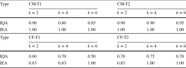
|
Type |
CM-T1 |
CM-T2 |
||||
|---|---|---|---|---|---|---|
|
|
|
|
|
|
|
|
|
IQA |
0.90 |
0.80 |
0.85 |
0.90 |
0.90 |
0.95 |
|
IEA |
1.00 |
1.00 |
1.00 |
1.00 |
1.00 |
1.00 |


|
Type |
CF-T1 |
CF-T2 |
||||
|---|---|---|---|---|---|---|
|
|
|
|
|
|
|
|
|
IQA |
0.60 |
0.70 |
0.50 |
0.70 |
0.75 |
0.70 |
|
IEA |
0.83 |
0.83 |
1.00 |
0.83 |
1.00 |
1.00 |


To see if role 2 is rational in their thinking, Table 17 in Appendix A.1 incorporates the average transfer
 from role 1 to role 2 in T2 into their payoffs in CF. It shows that X is a dominant action for role 2 when
 , and (X, X) is a payoff dominant equilibrium when
 . Furthermore, if role 2 expects that role 1’s action choice is given by its empirical frequency, X is his uniquely optimal action for every k.Footnote 39
In T1, we also have subjects of both roles whose action choice either is constant for every k, or switches once as k goes up. We call a subject type TX1 if his choices are either
 ,
,
 , or
, or
 as k increases from
 in T1. On the other hand, we call a subject type TY1 if his choices are either
 ,
,
 , or
, or
 as k increases from
 in T1.Footnote 40 It is worth noting that the two types cover more than 90% of all cases.Footnote 41 Table 9 shows the likelihood of action X in T1 and T2 by types TX1 and TY1.Footnote 42 As seen, type TX1 of either role chooses X most of the time in both T1 and T2 for each k. On the other hand, the change in the likelihood of X by type TY1 is dramatic. While by definition they never choose X at
 in T1, they choose X more than 60% of the time in T2.Footnote 43 Table 9 also hints at the possible mechanism behind Observation Footnote 2.2 on the effect of inequality on the action choice. As seen, type TY1 in CM-T1 sharply decreases the choice of X as k goes up, whereas TX1 is mostly unresponsive to the change in k. We can interpret the negative impact of k on X in CM-T1 as resulting from the inequality averse response by TY1. In CF-T1, on the other hand, TY1 and TX1 move in the opposite directions as k goes up, offsetting the impact of k.
Observation 5
Between T1 and T2, the increase in the choice of X by both roles 1 and 2 is mostly due to type TY1 who responds to increased inequality with the choice of Y in T1. In T2, the choice of X by role 2 is motivated by the anticipation of role 1’s choice of X and positive transfer.
Table 9 Rate of action X by T1 types
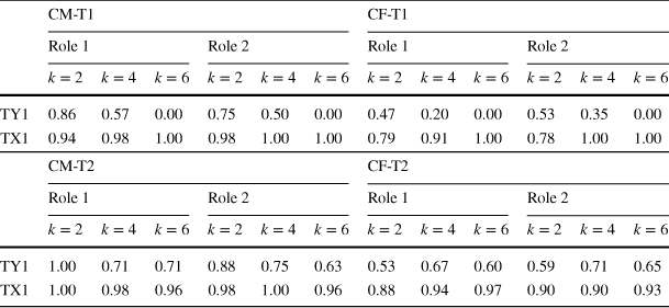
|
CM-T1 |
CF-T1 |
|||||||||||
|---|---|---|---|---|---|---|---|---|---|---|---|---|
|
Role 1 |
Role 2 |
Role 1 |
Role 2 |
|||||||||
|
|
|
|
|
|
|
|
|
|
|
|
|
|
|
TY1 |
0.86 |
0.57 |
0.00 |
0.75 |
0.50 |
0.00 |
0.47 |
0.20 |
0.00 |
0.53 |
0.35 |
0.00 |
|
TX1 |
0.94 |
0.98 |
1.00 |
0.98 |
1.00 |
1.00 |
0.79 |
0.91 |
1.00 |
0.78 |
1.00 |
1.00 |


|
CM-T2 |
CF-T2 |
|||||||||||
|---|---|---|---|---|---|---|---|---|---|---|---|---|
|
Role 1 |
Role 2 |
Role 1 |
Role 2 |
|||||||||
|
|
|
|
|
|
|
|
|
|
|
|
|
|
|
TY1 |
1.00 |
0.71 |
0.71 |
0.88 |
0.75 |
0.63 |
0.53 |
0.67 |
0.60 |
0.59 |
0.71 |
0.65 |
|
TX1 |
1.00 |
0.98 |
0.96 |
0.98 |
1.00 |
0.96 |
0.88 |
0.94 |
0.97 |
0.90 |
0.90 |
0.93 |


How does the difference in behavior in T1 translate to the difference in the transfer decisions in T2? For each role 1 subject, let his reciprocation index r be defined by

Each role 1 subject experienced (X, X) up to six times, and we call role 1 strongly reciprocating (SR) if
 , weakly reciprocating (WR) if
 , and non-reciprocating (NR) if
 . Table 19 in Appendix A.1 shows overall downgrading of reciprocity types going from CF-T2 to CM-T2: Nearly half of type SR in CF-T2 become NR in CM-T2, while few type NR in CF-T2 become SR in CM-T2. Table 10 shows the relationship between the type classification in T1 (i.e., TX1 and TY1 for role 1) and reciprocity types in T2. In CF-T2, the distribution of reciprocity types is almost identical between TY1 and TX1 with an even split between SR and NR. On the other hand, in CM-T2, nearly two-thirds of TX1 are NR, while it is much less likely that TY1 becomes NR. This shows that TY1 and TX1 are equally likely to reciprocate role 2’s choice of X accompanied by payoff sacrifice, but that TX1 is more likely to ignore 2’s choice of X if not accompanied by payoff sacrifice. In other words, TX1 and TY1 are different in the perception of kindness by role 2 that has led to the increase in their own payoff.
Table 10 T1 types and reciprocity types in T2

|
CM-T2 |
CF-T2 |
||||||
|---|---|---|---|---|---|---|---|
|
SR |
WR |
NR |
SR |
WR |
NR |
Other |
|
|
TY1 |
5 |
0 |
2 |
5 |
1 |
5 |
4 |
|
TX1 |
12 |
9 |
31 |
16 |
3 |
15 |
0 |
|
Other |
1 |
2 |
0 |
7 |
2 |
4 |
0 |
Reciprocity type “other” refers to role 1 who didn’t experience (X, X)
Observation 6
1. The degree of reciprocation is stronger in CF-T2 than in CM-T2 even for the same subject.
2. Type TX1 tends to reciprocate role 2’s choice of X only when it is accompanied by self-sacrifice.
Observation Footnote 6.1 supports the reciprocity hypothesis Footnote 1b. Observation Footnote 6.2 suggests that role 1’s behavior in T1 can be related to the difference in reciprocity between CM and CF.
8 Conclusion
The analysis of the paper is based on data from the sessions which presented the payoff formula (1) in the instructions. Apart from these sessions, we also ran five sessions in which the instructions did not present the payoff formula.Footnote 44 Appendix A.3 reports some analysis that compares the results with and without the formula. Most notably, we observe that the inclusion of the formula had significantly positive impacts on the subjects’ action choice both in T1 and T2. In particular, inclusion of the formula increases the frequency of action X and increases the frequency of efficient coordination (X, X). These results suggest that inclusion of the formula raises the awareness of the externalities involved in decision making in the inequality games. We believe that such awareness of externalities is key to the inducement of social preferences including reciprocity.Footnote 45
How would our findings help inform policy making in the possible presence of coordination inefficiencies? First and foremost, our finding suggests the importance of a salient opportunity for ex post reciprocation. While we formulate reciprocation as direct payoff transfer, the interaction may as well take an alternative form as long as it is sufficiently intuitive. Second, as noted above, our analysis suggests the importance of making the parties aware of the externalities involved in their decision making. Third, we note that player 2 in the CF inequality games likely uses self-sacrifice to convey a credible message behind his action choice to player 1, and is confident that player 1 understands this message. The lack of such a message in the CM inequality games has reduced the effectiveness of the redistribution scheme.Footnote 46 This observation suggests that the policy should create a channel through which the parties can credibly convey the intention behind their action choice.
One interesting extension of the present work involves elicitation of beliefs before the play of the games. It would be interesting to find out beliefs about the other player’s action choice, and the amount of transfer they expect from the other player after the realization of each action profile. Although we have studied the redistribution scheme in the presence of inequality between the players, it is important to check its validity in other classes of games. In the BOS game, for example, we would expect that the redistribution scheme as proposed here is valid if the sum of payoffs at one NE is substantially higher than that at the other NE. If, on the other hand, both NE are equally efficient, then some modification to the scheme would be required. In view of the literature, communication may play a critical role in such an environment. Examining the validity of the scheme under various payoff specifications is a topic of future research.
Acknowledgements
We are very grateful to the Editor and a referee for the comments that led to a significant improvement of the paper. Financial support from the JSPS (Grant Numbers: 22330061, 23530216, 24330064, 24653048, 15K13006, 15H03328, 16H03597, 16K17088, 15H05728, 20H05631) and the Joint Usage/Research Center at ISER, Osaka University, and the International Joint Research Promotion Program of Osaka University is gratefully acknowledged.
Appendix
A.1 Tables
Table 11 Random effects logit regressions of action choice:

|
Model |
(1) |
(2) |
(3) |
(4) |
(5) |
(6) |
(7) |
|
|---|---|---|---|---|---|---|---|---|
|
All |
CM |
CF |
CM |
CM |
CF |
CF |
||
|
t2 |
-0.58 |
0.31 |
− 0.71*** |
Role |
− 0.07 |
0.60 |
0.38 |
− 0.25 |
|
(0.40) |
(0.67) |
(0.26) |
(0.65) |
(0.86) |
(0.23) |
(0.52) |
||
|
cf |
1.86*** |
k
|
0.92*** |
1.32** |
0.21 |
− 0.81* |
||
|
(0.30) |
(0.15) |
(0.60) |
(0.40) |
(0.48) |
||||
|
cf * t2 |
− 0.23 |
k
|
1.11*** |
1.57*** |
− 0.01 |
− 0.01 |
||
|
(0.37) |
(0.29) |
(0.58) |
(0.40) |
(0.50) |
||||
|
Role |
− 0.06 |
0.38 |
Role * k
|
− 0.77 |
1.90*** |
|||
|
(0.53) |
(0.23) |
(1.20) |
(0.65) |
|||||
|
Role * t2 |
− 0.65 |
− 0.44 |
Role * k
|
− 0.87 |
0.00 |
|||
|
(0.97) |
(0.37) |
(1.26) |
(0.63) |
|||||
|
1/round |
6.55 |
22.00*** |
5.22 |
1/round |
1.29** |
1.32*** |
− 0.12 |
− 0.12 |
|
− 5.94 |
(7.34) |
(6.62) |
(0.51) |
(0.46) |
(0.41) |
(0.44) |
||
|
Constant |
− 3.81*** |
− 6.05*** |
− 2.04*** |
Constant |
− 5.10*** |
− 5.51*** |
− 1.57*** |
− 1.31*** |
|
(0.73) |
(0.85) |
(0.60) |
(1.13) |
(0.94) |
(0.33) |
(0.36) |
||
|
Log-likelihood |
− 513.09 |
− 167.24 |
− 342.10 |
Log-likelihood |
− 106.22 |
− 105.93 |
− 206.11 |
− 201.55 |
|
#obs. |
1,488 |
744 |
744 |
#obs. |
372 |
372 |
372 |
372 |
|
#subjects |
124 |
124 |
124 |
#subjects |
124 |
124 |
124 |
124 |


Model (1) combines data from CM and CF whereas models (2)-(7) separate them. Independent variables:
 if CF,
 if T2,
 if role 1,
 if
if
 , and
, and
 if
if
 . The variable
 equals the inverse of the round number within each task block, and is included given that all other independent variables are dummies. *, ** and ***: significant at 10%, 5% and 1%, respectively. Robust standard errors clustered by session in parentheses
Table 12 Logit regressions of action profiles

|
Model |
(1) |
(2) |
(3) |
(4) |
(5) |
(6) |
|---|---|---|---|---|---|---|
|
All |
CM |
CF |
||||
|
Dep. var. |
|
|
|
|
|
|
|
t2 |
0.81*** |
0.68*** |
1.09 |
1.06 |
0.85*** |
0.80*** |
|
(0.23) |
(0.22) |
(0.79) |
(0.78) |
(0.33) |
(0.21) |
|
|
cf |
− 1.84*** |
− 1.45*** |
||||
|
(0.23) |
(0.16) |
|||||
|
cf*t2 |
0.29 |
0.15 |
||||
|
(0.38) |
(0.35) |
|||||
|
1/round |
− 0.37 |
− 0.40* |
− 0.64* |
− 0.45 |
0.02 |
− 0.13 |
|
(0.27) |
(0.21) |
(0.36) |
(0.36) |
(0.37) |
(0.39) |
|
|
k
|
− 0.90*** |
− 0.79*** |
0.00 |
0.23 |
||
|
(0.15) |
(0.13) |
(0.48) |
(0.55) |
|||
|
k
|
− 0.98*** |
− 0.85*** |
0.38 |
0.69** |
||
|
(0.24) |
(0.28) |
(0.45) |
(0.34) |
|||
|
t2*k
|
0.26 |
0.10 |
0.43 |
0.06 |
||
|
(0.96) |
(0.94) |
(0.79) |
(0.79) |
|||
|
t2*k
|
− 0.59 |
− 0.68 |
0.34 |
− 0.02 |
||
|
(0.68) |
(0.59) |
(0.49) |
(0.33) |
|||
|
Constant |
1.86*** |
1.84*** |
2.96*** |
2.78*** |
− 0.24 |
− 0.02 |
|
(0.20) |
(0.17) |
(0.31) |
(0.32) |
(0.34) |
(0.18) |
|
|
#obs |
744 |
744 |
372 |
372 |
372 |
372 |
|
Log likelihood |
− 374.40 |
− 377.83 |
− 136.58 |
− 136.81 |
− 233.66 |
− 232.96 |


Models (1) and (2) combine data from CM and CF whereas models (3)-(6) separate them. See Table 11 for the definitions of the independent variables. *, ** and ***: significant at 10%, 5% and 1%, respectively. Robust standard errors clustered by session in parentheses
Table 13 Mixed effects Tobit regressions of final payoffs
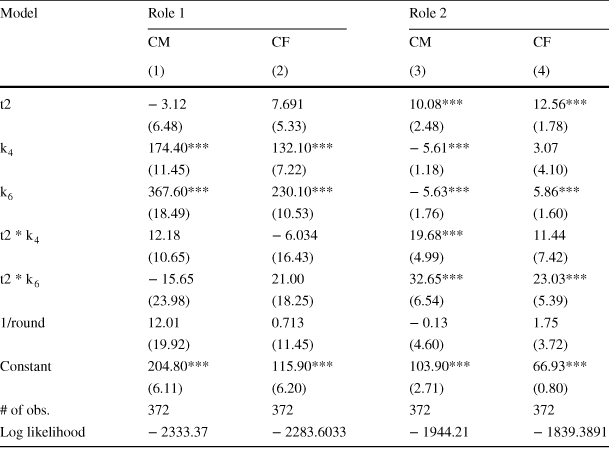
|
Model |
Role 1 |
Role 2 |
||
|---|---|---|---|---|
|
CM |
CF |
CM |
CF |
|
|
(1) |
(2) |
(3) |
(4) |
|
|
t2 |
− 3.12 |
7.691 |
10.08*** |
12.56*** |
|
(6.48) |
(5.33) |
(2.48) |
(1.78) |
|
|
k
|
174.40*** |
132.10*** |
− 5.61*** |
3.07 |
|
(11.45) |
(7.22) |
(1.18) |
(4.10) |
|
|
k
|
367.60*** |
230.10*** |
− 5.63*** |
5.86*** |
|
(18.49) |
(10.53) |
(1.76) |
(1.60) |
|
|
t2 * k
|
12.18 |
− 6.034 |
19.68*** |
11.44 |
|
(10.65) |
(16.43) |
(4.99) |
(7.42) |
|
|
t2 * k
|
− 15.65 |
21.00 |
32.65*** |
23.03*** |
|
(23.98) |
(18.25) |
(6.54) |
(5.39) |
|
|
1/round |
12.01 |
0.713 |
− 0.13 |
1.75 |
|
(19.92) |
(11.45) |
(4.60) |
(3.72) |
|
|
Constant |
204.80*** |
115.90*** |
103.90*** |
66.93*** |
|
(6.11) |
(6.20) |
(2.71) |
(0.80) |
|
|
# of obs. |
372 |
372 |
372 |
372 |
|
Log likelihood |
− 2333.37 |
− 2283.6033 |
− 1944.21 |
− 1839.3891 |


*, ** and ***Significant at 10%, 5% and 1%, respectively. Standard errors clustered by session in parentheses
Table 14 Role 1’s payoff in T2 conditional on the action profile in T1

|
T1 |
CF2 |
CF4 |
CF6 |
CM2 |
CM4 |
CM6 |
|---|---|---|---|---|---|---|
|
(X,X) |
132.429 |
231.393 |
384.857 |
206.855 |
405.438 |
560.208 |
|
(40.547) |
(106.812) |
(136.046) |
(34.280) |
(85.694) |
(166.431) |
|
|
28 |
28 |
35 |
55 |
48 |
48 |
|
|
0.001 |
0.002 |
0.002 |
0.0106 |
0.008 |
0.001 |
|
|
(X,Y) |
134.059 |
266.375 |
472.727 |
166.667 |
345.143 |
565.714 |
|
(34.965) |
(92.751) |
(13.484) |
(92.376) |
(137.914) |
(224.117) |
|
|
17 |
8 |
11 |
3 |
7 |
7 |
|
|
0 |
0.0004 |
0 |
0.1835 |
0.0016 |
0.001 |
|
|
(Y,X) |
99.800 |
275.286 |
322.444 |
214.500 |
366.667 |
548.333 |
|
(31.134) |
(65.198) |
(193.891) |
(9.713) |
(78.655) |
(153.677) |
|
|
15 |
21 |
9 |
4 |
6 |
6 |
|
|
0.9805 |
0.2954 |
0.1696 |
− |
− |
− |
|
|
(Y,Y) |
100.000 |
220.000 |
337.143 |
− |
438.000 |
460.000 |
|
(0.000) |
(88.318) |
(142.912) |
− |
− |
− |
|
|
2 |
5 |
7 |
− |
1 |
1 |
|
|
− |
− |
− |
− |
− |
− |
For each action profile in T1, the table lists the average payoff in T2 (line 1), standard deviations (line 2), the number of observations (line 3), and p-value of the hypothesis: “payoff in T1
 payoff in T2” by t-test (line 4). “−” implies insufficient observations
Table 15 Determinants of the size and likelihood of transfer
|
Model |
(1) |
(2) |
(3) |
(4) |
(5) |
(6) |
(7) |
(8) |
(9) |
|---|---|---|---|---|---|---|---|---|---|
|
All |
CM |
CF |
|||||||
|
Absolute |
Relative |
Likelihood |
Absolute |
Relative |
Likelihood |
Absolute |
Relative |
Likelihood |
|
|
2’s Y |
− 149.14*** |
− 0.28*** |
− 2.16*** |
||||||
|
(7.71) |
(0.01) |
(0.27) |
|||||||
|
cf |
23.54** |
0.08*** |
1.06*** |
||||||
|
(10.20) |
(0.02) |
(0.27) |
|||||||
|
2’s Y * cf |
28.21 |
0.132* |
− 0.23 |
||||||
|
(31.12) |
(0.08) |
(0.67) |
|||||||
|
k
|
40.83*** |
0.04** |
0.31 |
32.53** |
0.00 |
0.33 |
|||
|
(12.88) |
(0.02) |
(0.29) |
(15.68) |
(0.03) |
(0.42) |
||||
|
k
|
81.93*** |
0.07*** |
0.38 |
51.14*** |
0.00 |
0.56 |
|||
|
(13.29) |
(0.02) |
(0.26) |
(13.96) |
(0.03) |
(0.49) |
||||
|
1/round |
23.64 |
0.0469* |
0.81* |
46.44** |
0.10*** |
1.48*** |
23.92 |
− 0.01 |
0.16 |
|
(18.79) |
(0.03) |
(0.48) |
(19.81) |
(0.03) |
(0.55) |
(22.00) |
(0.05) |
(0.79) |
|
|
Constant |
− 48.33*** |
− 0.10*** |
− 1.22*** |
− 134.15*** |
− 0.20*** |
− 2.00*** |
− 54.43** |
− 0.03 |
− 0.62 |
|
(18.26) |
(0.04) |
(0.37) |
(13.34) |
(0.02) |
(0.38) |
(24.99) |
(0.05) |
(0.70) |
|
|
#obs. |
335 |
335 |
335 |
179 |
179 |
179 |
156 |
156 |
156 |
|
Log-likelihood |
− 808.31 |
− 17.03 |
− 157.29 |
− 379.61 |
− 23.88 |
− 87.71 |
− 432.53 |
− 11.46 |
− 88.52 |


Models (1), (2), (4), (5), (7) and (8) are the mixed effects Tobit regressions of the relative and absolute transfer amounts, whereas (3), (6) and (9) are the random effects probit regressions of the likelihood
 of positive transfer. The variable “2’s Y”
 if role 2’s action is Y. *, ** and ***Significant at 10%, 5% and 1%, respectively. Robust standard errors clustered by session in parentheses
Table 16 Tobit regressions of the payoff ratio

|
Variables |
(1) |
(2) |
(3) |
(4) |
(5) |
(6) |
|---|---|---|---|---|---|---|
|
CM |
CM |
CM |
CF |
CF |
CF |
|
|
t2 |
− 0.51*** |
− 0.51*** |
− 0.17*** |
− 0.47*** |
− 0.47*** |
− 0.37*** |
|
(0.15) |
(0.16) |
(0.05) |
(0.15) |
(0.11) |
(0.06) |
|
|
k4 |
1.64*** |
1.79*** |
1.51*** |
1.59*** |
||
|
(0.18) |
(0.16) |
(0.12) |
(0.18) |
|||
|
k6 |
3.36*** |
3.73*** |
2.80*** |
2.85*** |
||
|
(0.24) |
(0.30) |
(0.13) |
(0.05) |
|||
|
1/round |
0.88 |
0.29 |
0.26 |
− 0.87 |
− 0.01 |
− 0.05 |
|
(0.77) |
(0.50) |
(0.40) |
(0.85) |
(0.11) |
(0.15) |
|
|
t2 * k4 |
− 0.28 |
− 0.17 |
||||
|
(0.20) |
(0.17) |
|||||
|
t2 * k6 |
− 0.73** |
− 0.11 |
||||
|
(0.35) |
(0.27) |
|||||
|
Constant |
3.51*** |
2.09*** |
1.93*** |
3.98*** |
2.21*** |
2.18*** |
|
(0.09) |
(0.28) |
(0.12) |
(0.34) |
(0.06) |
(0.08) |
|
|
Log likelihood |
− 794.54 |
− 681.63 |
− 679.59 |
− 768.93 |
− 686.67 |
− 686.56 |
|
#obs |
372 |
372 |
372 |
372 |
372 |
372 |
|
#subject pairs |
62 |
62 |
62 |
62 |
62 |
62 |
*, ** and ***Significant at 10%, 5% and 1%, respectively. Robust standard errors clustered by session in parentheses
Table 17 Payoffs incorporating the average transfer from role 1:

|
CF2 |
CF4 |
CF6 |
||||||||||||
|---|---|---|---|---|---|---|---|---|---|---|---|---|---|---|
|
X (51) |
Y (11) |
X (52) |
Y (10) |
X (52) |
Y (10) |
|||||||||
|
X(48) |
149.1, |
90.9 |
53.3, |
26.7 |
X(53) |
292.1, |
107.9 |
60, |
20 |
X(55) |
437.6, |
122.4 |
59.7, |
20.3 |
|
Y(14) |
95.4, |
64.6 |
100, |
100 |
Y(9) |
244.3, |
75.8 |
100, |
100 |
Y(7) |
376, |
104 |
100, |
100 |
#observations in parentheses
Table 18 Types in T1 and T2

|
CM |
CF |
|||||||||||
|---|---|---|---|---|---|---|---|---|---|---|---|---|
|
Role 1 |
Role 2 |
Role 1 |
Role 2 |
|||||||||
|
TY2 |
TX2 |
Other |
TY2 |
TX2 |
Other |
TY2 |
TX2 |
Other |
TY2 |
TX2 |
Other |
|
|
TY1 |
2 |
4 |
1 |
2 |
4 |
2 |
6 |
9 |
0 |
5 |
9 |
3 |
|
TX1 |
2 |
49 |
1 |
2 |
48 |
0 |
1 |
32 |
1 |
2 |
34 |
5 |
|
Other |
0 |
3 |
0 |
1 |
3 |
0 |
0 |
12 |
1 |
1 |
3 |
0 |
Table 19 Reciprocity types in CM-T2 and CF-T2

|
CM-T2 |
|||||
|---|---|---|---|---|---|
|
SR |
WR |
NR |
Other |
||
|
CF-T2 |
SR |
14 |
3 |
11 |
0 |
|
WR |
2 |
2 |
2 |
0 |
|
|
NR |
1 |
5 |
18 |
0 |
|
|
Other |
1 |
1 |
2 |
0 |
|
Type “other” refers to role 1 who didn’t experience (X, X)
A.2 Figures
Fig. 4 Cumulative distributions of total payoffs in T1 and T2: CM (left) and CF (right)
Fig. 5 Final payoffs
 in CM (left) and CF (right): role 1 (dark) and role 2 (light)
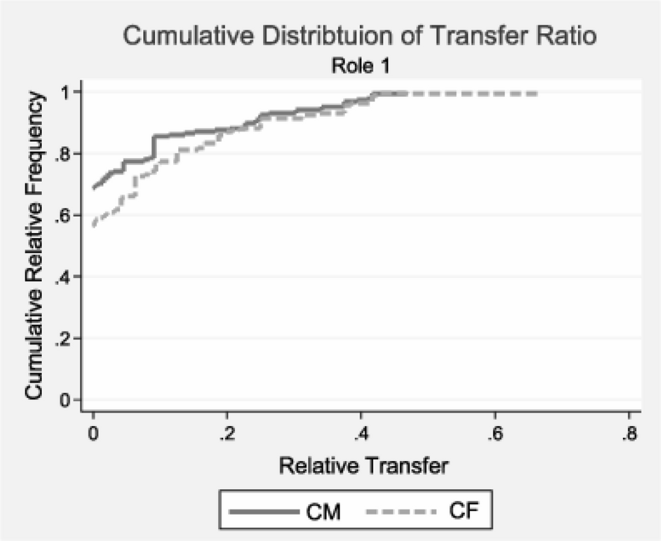
Fig. 6 Cumulative distributions of relative transfer by role 1 subjects
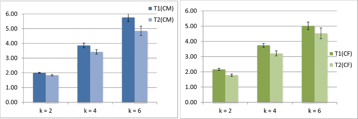
Fig. 7 Final payoff ratios
 in CM (left) and CF (right): T1 (dark) and T2 (light)
A.3 Effect of the Payoff formula in the instructions
This section examines the effects of including the payoff formula (1) in the instructions. There are a total of 106 subjects who participated in five sessions without the payoff formula but with the same task sequence as in the main experiments. Tables 20 and 21 describe the frequency of action Y by each role and the frequency of each action profile, respectively, in T1 and T2 with and without the payoff formula. We observe that role 1 chooses Y less often in every game with the formula, and that role 2 does so in four out of six games (CF2 and CM6). The effect is stronger in T2. In the case of action profiles, the efficient coordination profile (X, X) increases with the formula in every game, whereas the inefficient coordination profile decreases or does not change with the formula in every game. Again, these effects are generally stronger in T2. As seen in logit regressions reported in Tables 22 and 23, many of these changes are significant. In terms of transfer, the inclusion of the payoff formula also has positive impact on the average transfer by role 1 as seen in the Tobit regressions reported in Table 24.
On the other hand, the redistribution scheme increases the choice of X even without the formula: Going from T1 to T2, the rate of X increases by 6.8 percentage points in CM (83%
 89.3% for role 1 and 83%
 90.3% for role (2), and by 13.2 percentage points in CF (57.3%
 67.3% for role 1 and 65.3%
 81.7% for role (2). However, the increase is smaller than the corresponding number with the formula reported in Sect. 6.2.
Table 20 Frequencies of Y with and without formula

|
Role 1 |
Role 2 |
|||||||||||
|---|---|---|---|---|---|---|---|---|---|---|---|---|
|
T1 |
CF2 |
CF4 |
CF6 |
CM2 |
CM4 |
CM6 |
CF2 |
CF4 |
CF6 |
CM2 |
CM4 |
CM6 |
|
Without |
0.34 |
0.51 |
0.43 |
0.19 |
0.15 |
0.17 |
0.38 |
0.28 |
0.38 |
0.09 |
0.21 |
0.21 |
|
53 |
(0.07) |
(0.07) |
(0.07) |
(0.54) |
(0.05) |
(0.05) |
(0.07) |
(0.06) |
(0.07) |
(0.04) |
(0.06) |
(0.06) |
|
With |
0.27 |
0.42 |
0.27 |
0.06 |
0.11 |
0.11 |
0.31 |
0.21 |
0.31 |
0.05 |
0.13 |
0.13 |
|
62 |
(0.06) |
(0.06) |
(0.06) |
(0.03) |
(0.04) |
(0.04) |
(0.06) |
(0.05) |
(0.06) |
(0.03) |
(0.04) |
(0.04) |
|
T2 |
||||||||||||
|
Without |
0.38 |
0.26 |
0.34 |
0.06 |
0.13 |
0.13 |
0.17 |
0.17 |
0.21 |
0.09 |
0.09 |
0.11 |
|
53 |
(0.07) |
(0.06) |
(0.07) |
(0.03) |
(0.05) |
(0.05) |
(0.05) |
(0.05) |
(0.06) |
(0.04) |
(0.04) |
(0.04) |
|
With |
0.23 |
0.15 |
0.11 |
0.00 |
0.05 |
0.06 |
0.18 |
0.16 |
0.16 |
0.05 |
0.05 |
0.10 |
|
62 |
(0.05) |
(0.04) |
(0.04) |
(0.00) |
(0.03) |
(0.03) |
(0.05) |
(0.05) |
(0.04) |
(0.03) |
(0.03) |
(0.04) |
Standard errors in parentheses
Table 21 Action profiles with and without formula

|
CF2 |
CF4 |
CF6 |
|||||
|---|---|---|---|---|---|---|---|
|
Without |
With |
Without |
With |
Without |
With |
||
|
T1 |
(X, X) |
0.42 |
0.45 |
0.32 |
0.45 |
0.38 |
0.53 |
|
(X, Y) |
0.25 |
0.27 |
0.17 |
0.13 |
0.19 |
0.19 |
|
|
(Y, X) |
0.21 |
0.24 |
0.40 |
0.34 |
0.25 |
0.16 |
|
|
(Y, Y) |
0.13 |
0.03 |
0.11 |
0.08 |
0.19 |
0.11 |
|
|
Fisher’s test |
0.365 |
0.542 |
0.307 |
||||
|---|---|---|---|---|---|---|---|
|
T2 |
(X, X) |
0.53 |
0.63 |
0.60 |
0.71 |
0.55 |
0.76 |
|
(X, Y) |
0.09 |
0.15 |
0.13 |
0.15 |
0.11 |
0.13 |
|
|
(Y, X) |
0.30 |
0.19 |
0.23 |
0.13 |
0.25 |
0.08 |
|
|
(Y, Y) |
0.08 |
0.03 |
0.04 |
0.02 |
0.09 |
0.03 |
|
Fisher’s test |
0.32 |
0.459 |
0.033 |
||||
|---|---|---|---|---|---|---|---|
|
CM2 |
CM4 |
CM6 |
|||||
|
T1 |
(X, X) |
0.77 |
0.89 |
0.64 |
0.77 |
0.64 |
0.77 |
|
(X, Y) |
0.04 |
0.05 |
0.21 |
0.11 |
0.19 |
0.11 |
|
|
(Y, X) |
0.13 |
0.06 |
0.15 |
0.10 |
0.15 |
0.10 |
|
|
(Y, Y) |
0.06 |
0.00 |
0.00 |
0.02 |
0.02 |
0.02 |
|
|
Fisher’s test |
0.145 |
0.274 |
0.472 |
||||
|---|---|---|---|---|---|---|---|
|
T2 |
(X, X) |
0.87 |
0.95 |
0.81 |
0.90 |
0.79 |
0.84 |
|
(X, Y) |
0.08 |
0.05 |
0.06 |
0.05 |
0.08 |
0.10 |
|
|
(Y, X) |
0.04 |
0.00 |
0.09 |
0.05 |
0.09 |
0.06 |
|
|
(Y, Y) |
0.02 |
0.00 |
0.04 |
0.00 |
0.04 |
0.00 |
|
|
Fisher’s test |
0.254 |
0.318 |
0.409 |
Table 22 Random effects logit regressions of action choice Y with and without formula

|
Variables |
(1) |
(2) |
(3) |
(4) |
(5) |
(6) |
(7) |
(8) |
|---|---|---|---|---|---|---|---|---|
|
CF role1 |
CF role1 |
CM role1 |
CM role1 |
CF role2 |
CF role2 |
CM role2 |
CM role2 |
|
|
Formula |
− 1.141** |
− 0.506 |
− 1.386*** |
− 0.855* |
− 0.825** |
− 0.445 |
− 1.038 |
− 0.749 |
|
(0.50) |
(0.52) |
(0.46) |
(0.45) |
(0.38) |
(0.36) |
(0.69) |
(0.71) |
|
|
t2 |
− 0.057 |
− 0.042 |
− 0.0808** |
− 0.0699** |
− 0.128*** |
− 0.118*** |
− 0.0630** |
− 0.0564* |
|
(0.05) |
(0.05) |
(0.03) |
(0.03) |
(0.03) |
(0.03) |
(0.03) |
(0.03) |
|
|
1/round |
0.842*** |
0.893*** |
1.185** |
1.227** |
− 1.062*** |
− 1.082*** |
− 0.376 |
− 0.347 |
|
(0.30) |
(0.32) |
(0.60) |
(0.57) |
(0.35) |
(0.38) |
(0.70) |
(0.70) |
|
|
t2 * formula |
− 1.405*** |
− 1.371*** |
− 0.804*** |
− 0.625 |
||||
|
(0.31) |
(0.39) |
(0.16) |
(0.61) |
|||||
|
Constant |
− 0.937** |
− 1.035** |
− 3.442*** |
− 3.546*** |
− 0.552 |
− 0.585 |
− 2.522*** |
− 2.566*** |
|
(0.46) |
(0.47) |
(0.63) |
(0.64) |
(0.36) |
(0.37) |
(0.61) |
(0.64) |
|
|
Log likelihood |
− 351.95 |
− 342.23 |
− 178.54 |
− 175.15 |
− 332.86 |
− 329.45 |
− 198.85 |
− 197.88 |
|
#obs |
690 |
690 |
690 |
690 |
690 |
690 |
690 |
690 |
|
#subjects |
115 |
115 |
115 |
115 |
115 |
115 |
115 |
115 |
The variable
 for sessions with the formula. *, ** and ***Significant at 10%, 5% and 1%, respectively. Robust standard errors clustered by session in parentheses
Table 23 Logit regressions of action profiles with and without formula
|
Variables |
(1) |
(2) |
(3) |
(4) |
(5) |
(6) |
(7) |
(8) |
|---|---|---|---|---|---|---|---|---|
|
CF yy |
CF yy |
CM yy |
CM yy |
CF xx/yy |
CF xx/yy |
CM xx/yy |
CM xx/yy |
|
|
Formula |
− 1.428*** |
− 0.950* |
− 1.727** |
− 0.99 |
0.417** |
0.02 |
0.918** |
0.596 |
|
(0.54) |
(0.56) |
(0.83) |
(0.86) |
(0.17) |
(0.18) |
(0.37) |
(0.37) |
|
|
t2 |
− 0.09 |
− 0.08 |
0.00 |
0.01 |
0.04 |
0.03 |
0.0766*** |
0.0695*** |
|
(0.07) |
(0.07) |
(0.05) |
(0.05) |
(0.03) |
(0.03) |
(0.01) |
(0.01) |
|
|
1/round |
− 1.563*** |
− 1.637*** |
1.405** |
1.416** |
− 0.431** |
− 0.442** |
− 0.113 |
− 0.129 |
|
(0.42) |
(0.43) |
(0.70) |
(0.65) |
(0.20) |
(0.20) |
(0.38) |
(0.36) |
|
|
t2 * formula |
− 1.303*** |
Omitted |
0.772*** |
0.696** |
||||
|
(0.30) |
(0.21) |
(0.27) |
||||||
|
Constant |
− 2.006*** |
− 2.045*** |
− 4.784*** |
− 4.832*** |
0.340 |
0.383* |
1.395*** |
1.432*** |
|
(0.57) |
(0.58) |
(0.55) |
(0.56) |
(0.22) |
(0.22) |
(0.51) |
(0.52) |
|
|
Log likelihood |
− 166.33 |
− 163.64 |
− 51.63 |
− 50.20 |
− 456.03 |
− 450.20 |
− 298.47 |
− 296.31 |
|
#obs |
690 |
690 |
690 |
504 |
690 |
690 |
690 |
690 |
|
#subjects |
115 |
115 |
115 |
115 |
115 |
115 |
115 |
115 |
*, ** and ***Significant at 10%, 5% and 1%, respectively. Standard errors clustered by session in parentheses
Table 24 Mixed effects Tobit regressions of transfer with and without formula

|
Variables |
(1) |
(2) |
(3) |
(4) |
(5) |
(6) |
(7) |
(8) |
|---|---|---|---|---|---|---|---|---|
|
Conditional on (X, X) |
||||||||
|
CF |
CF |
CM |
CM |
CF |
CF |
CM |
CM |
|
|
Formula |
− 6.332 |
− 31.94* |
− 13.3 |
− 51.41** |
− 5.67 |
− 24.79 |
− 15.23 |
− 57.88** |
|
(7.94) |
(18.05) |
(15.17) |
(25.64) |
(6.33) |
(17.52) |
(13.68) |
(24.27) |
|
|
1/round |
9.765 |
10.08 |
41.75*** |
41.87*** |
7.939 |
8.215 |
36.62** |
36.74** |
|
(13.48) |
(13.49) |
(13.96) |
(13.97) |
(15.30) |
(15.32) |
(14.67) |
(14.65) |
|
|
Role |
70.99*** |
50.22*** |
82.77*** |
50.53** |
80.93*** |
63.55*** |
81.71*** |
45.27** |
|
(14.68) |
(15.36) |
(18.61) |
(19.64) |
(16.04) |
(16.76) |
(19.98) |
(22.07) |
|
|
Role * formula |
41.15** |
63.76*** |
31.21 |
71.34*** |
||||
|
(20.47) |
(23.46) |
(23.02) |
(25.14) |
|||||
|
Constant |
− 89.54*** |
− 77.02*** |
− 156.2*** |
− 136.8*** |
− 83.46*** |
− 73.09*** |
− 144.6*** |
− 122.9*** |
|
(16.97) |
(16.65) |
(24.65) |
(24.58) |
(19.21) |
(19.90) |
(22.29) |
(22.71) |
|
|
− 1196.78 |
− 1194.73 |
− 1026.13 |
− 1024.40 |
− 865.89 |
− 864.96 |
− 943.98 |
− 941.82 |
|
|
Observations |
690 |
690 |
690 |
690 |
438 |
438 |
596 |
596 |
|
Number of groups |
230 |
230 |
230 |
230 |
200 |
200 |
225 |
225 |
*, ** and ***Significant at 10%, 5% and 1%, respectively.
 if role 1. Standard errors clustered by session in parentheses
A.4 Proofs
Proof of Proposition 1
The utility function
 is concave in the own transfer
 so that the first-order condition fully characterizes the solution to the maximization problem. In particular, the solution is either at a corner (
 or
or
 ) or in the interior (
 ). When
 , we cannot have both
 and
and
 as interior solutions. The first-order condition for
 against
 or
or
 then yields the relationship between
 and
and
 in (4).
Reasoning for Hypothesis Footnote 1 is as follows:
1a. When
 and
,
and
since
. It follows that
and
by (4) and hence that the payoff profile including the SPE transfer at
is given by
. Hence, when
and
, then player 2’s choice of Y is strictly dominated and (X, X) is the unique SPE action profile. On the other hand, when
or
, (X, X) and (Y, Y) are both SPE action profiles. See Table 25.
and
,
and
since
. It follows that
and
by (4) and hence that the payoff profile including the SPE transfer at
is given by
. Hence, when
and
, then player 2’s choice of Y is strictly dominated and (X, X) is the unique SPE action profile. On the other hand, when
or
, (X, X) and (Y, Y) are both SPE action profiles. See Table 25.1b. By Fig. 1, at most one player i chooses
when
. If in addition
, then
while
if
and
if
. Since
implies
,
if and only if
or (Y, X). Regarding the comparison between CM-T2 and CF-T2, note that at
, player 1 chooses
if
in CM and
in CF. Hence, if
and
, player 1 chooses
at
only in CF.1c. When
,
if
. Since we specify
to be independent of the degree k of inequality in each class of games,
is also independent of k. This further implies that the action choice is independent of k as well in each class of games.


Table 25 Payoff profiles including SPE transfer


|
CM |
CF |
||||||||
|---|---|---|---|---|---|---|---|---|---|
|
X |
Y |
X |
Y |
||||||
|
X |
|
|
b, |
|
X |
|
|
b, |
|
|
Y |
|
|
a, |
a |
Y |
|
|
a, |
a |


Equilibrium under distributive social preferences
Let
 denote player i’s optimal choice in the dictator task T0, and
 and
and
 denote the set of (pure) NE and SPE action profiles in the inequality game G in tasks T1 and T2, respectively.
(1) Inefficiency aversion
In T0, the optimal action for player 1 is
 regardless of
 , and for player 2,
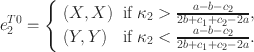
In T1,

Since the threshold
 decreases as
 increases (or
 increases), (7) implies that (X, X) is the unique NE for a larger set of
 for a larger k, implying Hypothesis Footnote 2c.Footnote 47 In T2, the transfer equals zero at any action profile and the set of SPE action profiles is as given in (7):
 . We hence have Hypotheses Footnote 2a and Footnote 2b.
(2) Inequality aversion
In T0,

and

In T1,
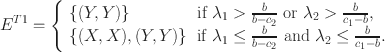
Since the threshold
 decreases as
 increases (or k increases), (Y, Y) is the unique NE for a larger set of
 for a larger k, implying the first part of Hypothesis Footnote 3c. In T2, if
 , then no transfer takes place in SPE, and the SPE action profile in stage 1 is the same as in T1:
 . If
. If
 , then (x, t) is an SPE if and only if x is a NE of the following game of identical-interest:
|
P1
|
X |
Y |
||
|---|---|---|---|---|
|
v |
|
|
|
|
|
Y |
|
|
2a |
2a |


and the transfer function t in SPE satisfies

Hence, Hypothesis Footnote 3b as well as the second part of Hypothesis Footnote 3c hold. Furthermore,
Except for CF2,
 holds and hence (X, X) is the unique SPE action profile. This along with (8) implies that (X, X) is played more often in T2 than in T1 (Hypothesis Footnote 3a).


 c1>c2
c1>c2


 t=(t1,t2)
 (γ1,γ2)

 χ
χ

 (t¯1,t¯2)


 y=1{ai=Y}


 (g1-t¯1,g2+t¯1)


 ui
ui

 u1/u2
u1/u2


 σ
σ


 Open access