Sharing or gambling? On risk attitudes in social contexts

Stefan Grimm; Martin G. Kocher; Michal Krawczyk; Fabrice Le Lec

doi:10.1007/s10683-020-09690-8

Sharing or gambling? On risk attitudes in social contexts

Published online by Cambridge University Press: 14 March 2025

Michal Krawczyk and

Stefan Grimm*: Affiliation:
Department of Economics, LMU Munich, Geschwister-Scholl-Platz 1, 80539 Munich, Germany
Martin G. Kocher*: Affiliation:
Institute for Advanced Studies, Josefstaedter Str. 39, 1080 Vienna, Austria Department of Economics, University of Gothenburg, Gothenburg, Sweden Department of Economics, University of Vienna, Oskar-Morgenstern-Platz 1, 1090 Vienna, Austria
Michal Krawczyk*: Affiliation:
University of Warsaw, 44/50 Dluga St, 00-241 Warsaw, Poland
Fabrice Le Lec*: Affiliation:
Lille Economics and Management, University of Lille, Cité Scientifique, UMR CNRS 9221, 59491 Villeneuve d’Ascq, Lille, France
*: stefan.j.grimm@googlemail.com
martin.kocher@univie.ac.at
mkrawczyk@wne.uw.edu.pl
fabrice.lelec@univ.lille.fr

Article contents

Abstract
Introduction
Experimental design and procedures
Experimental results
Discussion
Conclusion
Funding
Footnotes
References

Rights & Permissions

Abstract

Decisions under risk are often embedded in a social context that we usually abstract from when studying decision-making in the laboratory. In contrast to that practice, our experiment investigates whether risk-taking is affected by social comparisons. In particular, we focus on situations where some amount of money has to be allocated to two parties: either the amount can be shared, or a random device allocates the entire amount to one of the parties. We find that the social context of the decision matters strongly: When participants are in a disadvantageous initial position compared to the other party, they select the risky option much more often than in a purely individual decision, identical in all other respects. Overall, we find that individuals are relatively more risk-seeking in the socially unfavorable domain than in isolation, in contrast to the favorable one, where we find no or little change in elicited risk attitudes in comparison to an isolated decision.

Keywords

Risk attitude Risk in social context Social comparison Experiment

JEL classification

A13: Relation of Economics to Social Values C91: Laboratory, Individual Behavior D81: Criteria for Decision-Making under Risk and Uncertainty

Type: Original Paper
Information: Experimental Economics , Volume 24 , Issue 4 , December 2021 , pp. 1075 - 1104

DOI: https://doi.org/10.1007/s10683-020-09690-8 [Opens in a new window]
Creative Commons: This is an Open Access article, distributed under the terms of the Creative Commons Attribution (CC-BY) license (http://creativecommons.org/licenses/by/4.0/), which permits unrestricted re-use, distribution, and reproduction in any medium, provided the original work is properly cited.
Copyright: Copyright © The Author(s) 2020

1 Introduction

Most decisions under risk take place in a social context. Other individuals than the decision-makers themselves are present or involved when decision-makers have to make choices under risk. In these situations, other individuals or their behavior may, directly or indirectly, influence the decision-maker and her decisions (Trautmann and Vieider Reference Trautmann, Vieider, Roeser, Hillerbrand, Sand and Peterson2012).Footnote ¹ One channel through which social context may affect decision under risk is the possibility of social comparison. Thus, the question of whether elicited risk attitudes are affected by the relative social position of the decision-maker arises. The existing empirical literature on this question is inconclusive, despite the ubiquity of day-to-day decisions under risk for which social comparisons are possible. Our paper analyzes the influence of the relative social position of a decision-maker on her elicited risk attitudes, using a new experimental protocol that allows for additional insights.

More specifically, we implement a laboratory experiment in which the decision-maker has to choose either to share a prize with another player according to a given distribution, or to gamble for the entire prize. The two options (sharing or gambling) are set to be equivalent in terms of expected payoff, and hence the choice between them provides a measure of risk attitude in a social context. By systematically varying the distribution of the prize as well as the probability to obtain it, we can systematically change the relative social position of the decision-maker vis-à-vis the other player and directly observe effects of the relative social position on risk-taking.

Our experiment reproduces, in a simplified manner, important aspects of situations that involve risk in a social context, especially those for which the total amount, endowment or resource distributed is constant. This corresponds to circumstances in which an individual can either favor a given distribution of financial resources and power, or take the chances of obtaining the entire prize herself. For instance, an executive can accept the proposed split of available funding between her and another manager’s project or argue that the company should focus on just one of them, with the risk of losing out. A political leader may have to choose between accommodating the current division of power between herself and a party rival or go for a shootout that will leave just one of the two standing. A poker player in a cash game can leave the table with current possessions or continue playing until all is lost or won. In any of these examples, not only the relative position (being ahead or behind) may affect the decision-maker’s inclination to take risk, but the mere fact of being in a social context may lead her to take more (or less) risk. To sum up, our setup involves the comparison of decisions on implementing a given distribution in a social context, when either being ahead or behind (favorable inequity or unfavorable inequity), and a control setting in which equivalent decisions are taken in isolation (i.e. without social context).

At least three effects established in the relevant literature may influence risk attitude through social comparisons. First, positional concerns (e.g., Charness et al. Reference Charness, Masclet and Villeval2013; Kuziemko et al. Reference Kuziemko, Buell, Reich and Norton2014) may provide additional utility to winners or reduce utility of losers. They may lead decisions makers to take more risk than they would do otherwise if there is a possibility to be ahead of another individual. Vice versa, they may lead decision-makers to be more cautious if gambling involves the possibility of falling behind. Second, decision-makers may feel gloating and envy with different intensity. That is, decision-makers subjectively value an additional dollar differently when being ahead than when catching up from behind. Bault et al. (Reference Bault, Coricelli and Rustichini2008) provide evidence for such an effect that may lead decision-makers to seek risky options that provide a chance of being ahead of others. Third, utility curvature may be different in the socially unfavorable domain (behind others) than in the socially favorable domain (ahead of others). Linde and Sonnemans (Reference Linde and Sonnemans2012) propose the idea of a social reference point applied to prospect theory (Kahneman and Tversky Reference Kahneman and Tversky1979; Tversky and Kahneman Reference Tversky and Kahneman1992) that would make decision-makers risk-averse in the favorable domain and risk-seeking in the unfavorable domain.

With regard to the general question of whether social comparisons affect risk-taking and, in particular, if so, in which direction, the existing experimental economics literature is quite inconclusive hitherto: Linde and Sonnemans (Reference Linde and Sonnemans2012) find, in contrast to their theoretical predictions, that decision-makers are more risk-seeking when being ahead of another individual. Bault et al. (Reference Bault, Coricelli and Rustichini2008) observe that decision-makers are slightly more risk-seeking for mixed lotteries in the social domain, i.e. with consequences in the socially favorable and the socially unfavorable domain. Bolton and Ockenfels (Reference Bolton and Ockenfels2010) as well as Gamba et al. (Reference Gamba, Manzoni and Stanca2017) in a real-effort task find, in contrast, that decision-makers are more risk-seeking when being behind another individual.Footnote ² In light of the existing mixed evidence, our experimental setting provides the following benefits: the design is parsimonious, it clearly identifies the effect of social comparisons, it varies systematically the relative positions of the decision-maker, and it compares (otherwise identical) decisions in a social environment and in isolation. Furthermore, it avoids confounding factors—sometimes present in other studies—such as (ex post) social preferences or specific peer effects (conformism).

Our main finding is that the number of risky choices is strongly affected by the social context. Subjects in our experiment are more risk-seeking when the deterministic option involves unfavorable inequity than in the same decision in isolation. In contrast, a favorable social context (when the deterministic option corresponds to favorable inequity) does not increase the willingness to take risks compared to an identical decision without social context. The analysis of individual behavior suggests that most of this asymmetry is driven by about two-thirds of experimental participants who very strongly exhibit this choice pattern of becoming more risk-seeking in what appears to be the social loss domain. The pattern is robust to various controls and sensitivity checks. A deeper inspection of our data suggests that neither a difference in the intensities of gloating and envy, on the one hand, nor a mere concern for being ahead in an ordinal ranking, on the other hand, can explain all aspects of the data pattern. Among the documented effects found in the literature, the difference in curvature in the favorable and unfavorable social domain seems the only explanation compatible with our data. In particular, the hypothesis that the other participant’s payoff plays the role of a (social) reference point, below which the decision-maker is risk-seeking (social loss domain) and above which she is risk-averse (social gain domain) seems to be consistent with the observed pattern.

The remainder of the paper is organized as follows: the next section presents the experimental design and procedures; Sect. 3 shows our results, and Sect. 4 discusses the results in light of the existing literature and existing theories of decision-making under risk. Section 5 concludes the paper.

2 Experimental design and procedures

The experiment consisted of five short parts: a series of risky choices in a social context; two dictator game decisions; a series of tasks to elicit individual risk preferences and potential loss aversion (in decisions without a social context); a series of risky choices without a social context (but different than in the part before); and the so-called ring test (the incentivized social value orientation questionnaire) to measure social value orientation.

2.1 Decision-making under risk in varying decision contexts

We use a within-subject design that allows us to compare decision-making under risk in a social context with decision-making under risk in a purely individual context. Since the decisions are identical with respect to the decision-maker's payoffs and probabilities, differences in decision-making between the individual and the social context can be attributed to the context in which the decisions took place.

In part 1 of the experiment, subjects faced tasks where €10 had to be allocated between the decision-maker and an anonymous receiver, both being present in the laboratory. Two options were available. The first one (OPTION A) was the deterministic (safe) option, which was the plain division of €10, i.e. the allocation (x, 10 − x) for a given x. The second one was the risky option (OPTION B), which was the social lottery where the decision-maker had a chance of x/10 of obtaining the entire €10 (and the receiver obtaining €0), while the receiver had the residual chance of (10 − x)/10 of getting €10 (and the decision-maker obtaining 0). The chances of winning €10 were thus mutually exclusive between the decision-maker and the receiver. The amount x was systematically varied to obtain nine different tasks, with x ranging from 1 to 9 in steps of 1. Table 1 displays all tasks subjects faced in part 1. Participants were asked whether they preferred Option A (henceforth also referred to as ‘the safe option’) or Option B (henceforth also ‘the risky option’). They could also indicate indifference (Option C). For that case, they were told that Option A or Option B would be implemented randomly with equal probability, realized through a draw of the computer. Each subject was asked to make a choice in every row of the table.

Table 1 Part 1—social context tasks

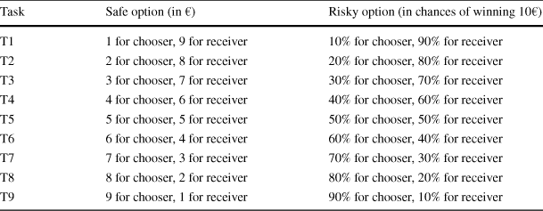
Task	Safe option (in €)	Risky option (in chances of winning 10€)
T1	1 for chooser, 9 for receiver	10% for chooser, 90% for receiver
T2	2 for chooser, 8 for receiver	20% for chooser, 80% for receiver
T3	3 for chooser, 7 for receiver	30% for chooser, 70% for receiver
T4	4 for chooser, 6 for receiver	40% for chooser, 60% for receiver
T5	5 for chooser, 5 for receiver	50% for chooser, 50% for receiver
T6	6 for chooser, 4 for receiver	60% for chooser, 40% for receiver
T7	7 for chooser, 3 for receiver	70% for chooser, 30% for receiver
T8	8 for chooser, 2 for receiver	80% for chooser, 20% for receiver
T9	9 for chooser, 1 for receiver	90% for chooser, 10% for receiver

In part 4 of the experiment subjects faced a task equivalent to part 1 of the experiment (see Table 2). However, now the choice was individual. That is, they had to decide between a safe payoff of €x and a lottery with probability x/10 of receiving €10 and probability (10 − x)/10 of receiving nothing. There was no other participant that was affected by the nine decisions taken in part 4. An indifference option (Option C) was also available, and the procedure was analogous to part 1.

Table 2 Part 4—individual context tasks

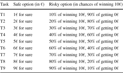
Task	Safe option (in €)	Risky option (in chances of winning 10€)
T1	1€ for sure	10% of winning 10€, 90% of getting 0€
T2	2€ for sure	20% of winning 10€, 80% of getting 0€
T3	3€ for sure	30% of winning 10€, 70% of getting 0€
T4	4€ for sure	40% of winning 10€, 60% of getting 0€
T5	5€ for sure	50% of winning 10€, 50% of getting 0€
T6	6€ for sure	60% of winning 10€, 40% of getting 0€
T7	7€ for sure	70% of winning 10€, 30% of getting 0€
T8	8€ for sure	80% of winning 10€, 20% of getting 0€
T9	9€ for sure	90% of winning 10€, 10% of getting 0€

By comparing decisions in part 1 and part 4 of the experiment, we can isolate attitudes towards risk in the social context and compare them to risk-taking in the individual context. Social context here simply means that another participant’s earnings were determined by the choices of the decision-maker.

2.2 Theoretical considerations

In the following we discuss theoretical considerations based on relevant assumptions for our setup. We formulate them as predictions, but not all of them can be tested rigorously in our experiment. Still, they help organizing our thoughts.Footnote ³

2.2.1 Self-interested expected utility maximizers

We first focus on the standard case where the decision-maker is self-interested and maximizes expected utility. The predictions are straightforward, given the assumption that decision-makers pay no attention to the other player’s outcome. T1 to T9 stand for the nine decisions in the social context, and T1i to T9i stand for the nine decisions without social context.

Prediction 1

(standard self-interest) If the decision-maker is a self-interested expected utility maximizer, each of her decisions in any of the tasks T1-T9 are the same as in the equivalent tasks in T1i-T9i.

Prediction 2

(standard self-interest—risk attitude) If the decision-maker is a self-interested expected utility maximizer with a concave (resp. convex) utility function, she chooses the safe (resp. risky) option in all the tasks T1-T9 and T1i-T9i.

In the absence of any regard to the other party’s prospect, the decision-maker’s preferences reduce to a dependence on the standard (individual) attitudes towards risk.

2.2.2 Definition of social risk attitude

In order to investigate whether risk attitudes vary depending on the social context, we require a formal and rigorous definition of social risk attitude. We propose to define social risk attitude as the preference between the deterministic (certain) combination of two social outcomes and its equivalent probabilistic combination. A socially risk-averse decision-maker will prefer to combine deterministic social outcomes to combining them probabilistically, while a social risk-seeking decision-maker will prefer the probabilistic combination.

Formally, let $x = (x_{1}, x_{2})$ and $y = (y_{1}, y_{2})$ be two generic social payoff vectors, with $x_{1}, x_{2}, y_{1,} y_{2} \in R$ . We restrict attention to the case of two decision-makers, the only one relevant for our experiment. For a given $α \in (0, 1)$ , the deterministic (certain) combination of $x$ and $y$ , denoted $α x + (1 - α) y$ , is given by (1):

(1)

α x + (1 - α) y = (α x_{1} + (1 - α) y_{1}, α x_{2} + (1 - α) y_{2})

On the other hand, the probabilistic combination of $x$ and $y$ for $p \in (0, 1)$ , denoted $p \otimes x \oplus (1 - p) \otimes y$ , is defined as the simple probabilistic mixture of $x$ and $y$ (Herstein and Milnor Reference Herstein and Milnor1953). Put differently, we have:

(2)

p \otimes x \oplus (1 - p) \otimes y = (p, (x_{1}, x_{2}); 1 - p, (y_{1,} y_{2}))

The probabilistic p-combination of $x$ and $y$ is just the lottery that gives $x$ with probability p and $y$ with probability 1−p. In what follows, we define risk aversion as $α x + (1 - α) y$ being preferred over $α \otimes x \oplus (1 - α) \otimes y$ , and risk seeking as the opposite case. Let the preference of the decision-makers on the mixture space on $R^{2}$ be asymmetric and negatively transitive, with $\sim$ defined as the usual indifference relation. Then, the general definition of social risk aversion (or social risk-seeking attitude) is quite straightforward:

Definition 1

(social risk attitude):

An agent is said to be socially risk-averse on a subset $S$ of $R^{2}$ and an interval $I \subset (0, 1)$ if, for all $x, y$ in $S$ , it holds that for any $α \in I$ :

α x + (1 - α) y ≻ α \otimes x \oplus (1 - α) \otimes y

An agent is said to be socially risk-seeking on $S$ if, for all $x, y$ in $S$ , it holds that for any $α \in (0, 1)$ :

α \otimes x \oplus (1 - α) \otimes y ≻ α x + (1 - α) y

It is easy to show that if the decision-maker is self-interested in the sense that she never takes into account the other party’s prospect or outcome, social risk attitude reduces to standard risk attitude over payoffs in $R$ . Yet, in general, decision-makers can obviously exhibit a rich domain of social risk attitudes, for instance being risk-seeking on some interval/domain and risk-averse on another. For example, an individual maximizing $x_{1} + b x_{2}^{a}$ is risk-neutral when only her own payoff is at stake but socially risk-seeking, risk-neutral, or socially risk-averse (depending on the value of a).

The purpose of the following discussion is to clarify these conditions and derive theoretical considerations for our setup.

2.2.3 Social risk attitude and (ex post) social preferencesFootnote ⁴

We want to emphasize that social risk attitude is conceptually distinct from social preferences, or more generally, ex post other-regarding considerations. Indeed, the intuition may suggest (wrongly) that the relative (ex post) payoff may generate adjustments in social risk attitude. To illustrate our point, consider a decision-maker with competitive preferences having to choe between $α \otimes x \oplus (1 - α) \otimes y$ and $α x + (1 - α) y$ , with $x = (M, 0)$ and $y = (0, M)$ , as in our experiment. Suppose now that the decision-maker has competitive preferences, i.e. her utility depends only on the difference between her payoff and the other party’s payoff. It is tempting to think that if $α x_{1} + (1 - α) y_{1}$ is below $α x_{2} + (1 - α) y_{2}$ , that is if the certain combination gives less to the decision-maker than to the other party, the decision-maker will prefer to take the gamble with the hope to reverse the (relative) outcomes. In fact, this intuition appears to be incorrect: Suppose for the sake of the argument that the decision-maker maximizes expected utility. What matters then is the utility of the relative position $(α x_{1} + (1 - α) y_{1}) - (α x_{2} + (1 - α) y_{2})$ to the expected utility of $(α, (x_{1} - x_{2}); 1 - α, (y_{1} - y_{2}))$ ; put differently it depends on $u ((α x_{1} + (1 - α) y_{1}) - (α x_{2} + (1 - α) y_{2}))$ , on the one hand, and $α u (x_{1} - x_{2}) + (1 - α) u (y_{1} - y_{2})$ , on the other hand. What matters is hence not the valence of the other party’s payoff or the valence of the difference in payoffs, but how the utility of the convex combination fares relatively to the expected utility of the corresponding lottery, that is whether the utility function is concave or convex on its relevant segment.

More generally, whatever the social motivations that enter the decision-maker’s utility (altruism, rivalry or competitive preferences, inequity aversion, etc.), what matters in the main experimental task is the relative position of the utility of $(α M, (1 - α) M)$ , not the ‘intensity’ of the preference for $(M, 0)$ over $(0, M)$ . Suppose, for instance, that $(M, 0) ≻ (α M, (1 - α) M) ≻ (0, M)$ ,Footnote ⁵ and set, without loss of generality, $u (M, 0) = 1$ and $u (0, M) = 0$ . Then, whether the decision-maker is socially risk-seeking or risk-averse in the experiment comes down to whether $u (α M, (1 - α) M)$ is greater than $α$ , that is, the convexity/concavity of $u$ on the segment $((M, 0), (0, M))$ .Footnote ⁶

In general, it is easy to show that if the partial derivative of the utility function with respect to the other party’s payoff is always of the same sign (monotonic social preferences), the decision-maker’s social risk attitude depends on the concavity/convexity of her utility over the relevant interval.

Prediction 3

(generic monotonic social preferences) The social risk attitude of a decision-maker with monotonic social preferences depends on the curvature (convexity/concavity) of her utility function.

In fact, the attitude towards social risk does not depend on the type of consideration for others that comes into play in the decision-maker’s preferences (such as inequity aversion, rivalry, maximin, etc.), but on the curvature of the corresponding utility function. This applies to all generic models of social preferences, such as inequity aversion, altruism, spitefulness, competitive preferences, quasi-maximin, etc.

2.2.4 Changes in social risk attitudes

Several studies have shown (or argued) that there are plausible motives for individuals to change risk attitude depending on the relative social situation. Bault et al. (2008) observe that for some specific lotteries and situations, decision-makers are willing to take more risks, and they conclude that gloating (the subjective benefit) from being ahead of the counterpart is stronger than the negative feeling generated by being behind the other party (envy). Linde and Sonnemans (Reference Linde and Sonnemans2010) assume that the other party’s payoff plays the role of a reference point in a model with a prospect theory flavor. This implies that decision-makers are risk-seeking in the (relative) loss domain (when behind) and risk-averse in the relative gain domain (when ahead). However, they do not find support for their model in an experiment. Another rationale for a change in social risk attitude is the general idea that being behind or ahead of another party generates a discrete change in satisfaction (of which last place aversion in Kuziemko et al.Reference Kuziemko, Buell, Reich and Norton2014, is a specific instance). Losing may generate a negative feeling (fixed in intensity), while winning may generate a positive one.

Existing models make similar generic predictions in terms of a possible change in social risk attitudes: Decision-makers tend to be more risk-seeking when $α$ is low (in the socially unfavorable case) than when $α$ is high (in the socially favorable case). In the following, we make some more precise predictions.

Prediction 4

(gloating larger than envy) A rival decision-maker with gloating larger than envy and a piece-wise linear utility will switch from social risk aversion for T6 to T9 ( $α > 0.5$ ) to a social risk-seeking attitude for T1 to T5 ( $α \leq 0.5$ ).

Consider the simplest case when utility is piece-wise linear in $x_{1} - x_{2}$ : $u (x_{1}, x_{2})$ = $(x_{1} - x_{2})$ if $x_{2} \geq x_{1}$ and $u (x_{1}, x_{2}) = γ (x_{1} - x_{2})$ if $x_{1} > x_{2}$ , with $γ > 1$ as the gloating parameter. Remember that the choice is between $u (α M, (1 - α) M)$ and $α u (M, 0) + (1 - α) u (0, M)$ in our experiment. If $α > 0.5$ , the safe option gives $u (α M, (1 - α) M) = γ (2 α - 1) M$ , while the risky option gives $α u (M, 0) + (1 - α) u (0, M) = α γ M - (1 - α) M < γ (2 α - 1) M$ . Hence, the decision-maker chooses the safe option. On the other hand, if $α \leq 0.5$ , the safe option gives $u (α M, (1 - α) M) = (2 α - 1) M$ , while the risky option gives $α u (M, 0) + (1 - α) u (0, M) = α γ M - (1 - α) M > (2 α - 1) M$ . Hence, the decision-maker chooses the risky option.

We now consider the case where the decision-maker obtains a utility bonus, whenever she earns more than the other party or obtains a utility malus whenever she earns less (see Online Appendix D.1 for the formal calculations).

Prediction 5

(discrete utility effect with social rank) Decision-makers with last-place aversion will choose the risky option more often in T1 to T4 than in T1i to T4i, and they will choose the safe option more often in T5 to T9 than in to T5i to T9i. Decision-makers with winning bonus utility will choose the risky option more often in T1 to T5 than in T1i to T5i, and they will choose the safe option more often in T6 to T9 than in T6i to T9i.

An interesting secondary prediction regarding the discrete effect of positional concerns is that their effects are maximal near $α = 0.5$ . As an illustration, consider a decision-maker with a winning bonus utility, in the case where $α < 0.5$ . The lower $α$ , the less likely s/he is to win and to get the bonus, hence the less attractive the risky option. Moreover, for a expected utility maximizer, the difference in expected utility between the safe and the risky option decreases linearly in $α$ . The exact mirror phenomenon holds for decision-makers with last-place aversion (once again, details are provided in Online Appendix D.1).

Now we consider a prospect theory model with social reference point, as suggested by Linde and Sonnemans (Reference Linde and Sonnemans2012). The intuition of the model is straightforward: as decision-makers are (roughly) risk-seeking in the loss domain and risk-averse in the gain domain, decision-makers will tend to take more risk in a socially disadvantageous situation than in a socially advantageous one. In order to keep the discussion tractable, we simplify the model by assuming a linear treatment of probabilities (see Online Appendix D.2 for the formal derivation).

Prediction 6

(simplified prospect theory) Prospect theory decision-makers will exhibit a risk-seeking attitude for T1 to T4 and risk aversion for T5 to T9, while showing risk aversion for T1i to T9i.

2.3 Experimental controls

The remaining parts of the experiment (parts 2, 3, and 5) were designed to measure social preferences, risk attitudes (independently) and potential loss aversion. More precisely, in part 2 of the experiment, subjects had to play two dictator games (Forsythe et al. Reference Forsythe, Horowitz, Savin and Sefton1994; Bolton et al. Reference Bolton, Zwick and Katok1998). The first was a regular dictator game with 10€ to be divided between the decision-maker (the dictator) and the receiver. The second allocation decision consisted of dividing chances (probabilities) to win 10€ (the ‘competitive probabilistic dictator game’ of Krawczyk and Le Lec Reference Krawczyk and Le Lec2010). For example, the dictator could decide that, with probability 70%, she will win 10€ and the other participant 0€, and otherwise (with probability 30%) the opposite would be implemented. Finally, participants had to indicate which of the two ‘games’ they preferred. The first game provides us with a control for outcome-based social concerns, while the second game speaks to preferences regarding procedural social concerns.

In part 3 of the experiment participants received a truncated and adapted Holt and Laury (Reference Holt and Laury2002) multiple choice list to independently estimate subjects’ risk attitudes with stakes comparable to the ones used in the main part of our experiment. This three-question version of the standard choice list contains the relevant choices in which the vast majorities of experimental subjects usually switch from safe to risky lotteries.Footnote ⁷ We also included three decisions that aim at assessing loss attitudes. Table 3 lists all choices in part 3 of the experiment.

Table 3 Part 3—risk and loss attitude choices

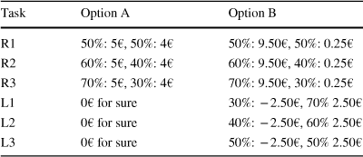
Task	Option A	Option B
R1	50%: 5€, 50%: 4€	50%: 9.50€, 50%: 0.25€
R2	60%: 5€, 40%: 4€	60%: 9.50€, 40%: 0.25€
R3	70%: 5€, 30%: 4€	70%: 9.50€, 30%: 0.25€
L1	0€ for sure	30%: − 2.50€, 70% 2.50€
L2	0€ for sure	40%: − 2.50€, 60% 2.50€
L3	0€ for sure	50%: − 2.50€, 50% 2.50€

Part 5 elicits social value orientation with the so-called ring test (Offerman et al. Reference Offerman, Sonnemans and Schram1996; van Lange et al. Reference Van Lange, De Bruin, Otten and Joireman1997; Brosig Reference Brosig2002; van Dijk et al. Reference Van Dijk, Sonnemans and van Winden2002). In this fully incentivized test, subjects have to make binary choices in 24 different allocation tasks (see Online Appendix A for details). In each task, a subject has to choose between two allocations that give money to herself and another (anonymous) recipient. The recipient stays the same in all 24 allocation tasks, and all 24 tasks are paid. Adding up the decisions in the 24 tasks yields a total sum of money allocated to oneself (x-amount) and to the recipient (y-amount). Using the ratio (x/y), one can assign a subject to one of eight categories of social orientation (individualism, altruism, cooperation, competition, martyrdom, masochism, sadomasochism, and aggression).

2.4 Experimental procedures

The experiment was conducted at the munich experimental laboratory for economic and social sciences (MELESSA) using z-tree (Fischbacher Reference Fischbacher2007) for programming and ORSEE (Greiner Reference Greiner2015) for recruitment. We ran nine sessions with a total of 216 subjects; mostly students from the University of Munich.Footnote ⁸ Subjects were allowed to participate in only one session.

Participants were asked to take all the choices described above. Their roles in parts 1 and 2 of the experiment—either decision-maker or receiver—were determined after the experiment, using the strategy method (Selten Reference Selten and Sauermann1967; Brandts and Charness Reference Brandts and Charness2011). Resolution of uncertainty was implemented and outcome information was given only at the very end of the entire experiment. Instructions for parts 1–4 were distributed and read aloud at the beginning of the experiment, and upon finishing part 4, instructions for part 5 were read and distributed. Subjects knew that there were exactly five parts from the beginning of the experiment. Two-thirds of participants faced choices in the order described above. For one third the order was reversed (on the request of a referee): They worked on the individual lotteries first (part 4 above), before the control choice lists (part 3 above), then played the dictator games (part 2 above) and answered the social lotteries, before receiving the instructions for the ring test.

To determine payoffs, subjects were randomly matched with another participant within the session. One subject in these matched pairs was always randomly selected for the role of decision-maker; the other was the receiver. For all pairs of participants, a random mechanism decided the payoff-relevant part from parts 1 to 4. If part 1 or 2 was chosen, another random mechanism then would decide which specific task within the part was to be implemented for both participants. If part 3 or 4 was chosen, the specific task to be implemented was determined for both participants separately. In addition to the payoff from this single decision out of parts 1 to 4, all subjects received their earnings from the ring test in part 5, which consisted of their payoff from their own choices and the payoff from the choices of the matched participants. Matching of participants in part 5 of the experiment was independent of the matching in parts 1 and 2. On top of these earnings, participants received a fixed payment for showing up on time. On average, participants earned 15.33€, and a session took about 50 min.

Participants were also asked to fill out a questionnaire after part 5, including a short description of motivations for decisions in the experiment and questions regarding socio-demographic characteristics. All design details and the procedural details were common knowledge among participants (see the instructions for all parts in Online Appendix B).

3 Experimental results

We will first have a look at aggregate results (Sect. 3.1), before analyzing the data on an individual level and taking into account the heterogeneity in responses (Sect. 3.2).

3.1 Aggregate results

An overview of the results from decision-making under risk in the social context (part 1 of the experiment) is shown in Fig.1. The aggregate pattern of risk-taking is roughly L-shaped, with subjects willing to take considerably more risk in unfavorable tasks where the expected payoff to the decision-maker is smaller than the expected payoff to the matched participant. The level of risk-taking reaches its lowest value at the equal split.

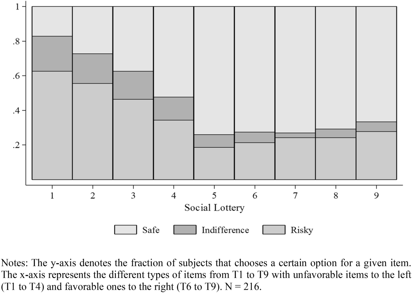
Fig. 1 Distribution of choices in the social context

The asymmetry between favorable and unfavorable situations is statistically significant. Leaving the case of the equal split aside for the moment, all comparisons between tasks corresponding to deterministic payoffs adding up to 10 (T1 vs. T9, T2 vs. T8, T3 vs. T7, and T4 vs. T6) suggest that the risky option is relatively more appealing, when the safe option implies unfavorable inequity. The differences are significant according to a Stuart-Maxwell test at the 1%-level. If we pool indifference with the risky option or with the safe option, McNemar’s tests remain significant at the 1%-level for either pooling version and for all comparisons. Looking at the unfavorable situations only, statistical tests support increasing risk-taking from the equal split towards the more unfavorable tasks. For all binary comparisons between the tasks in the unfavorable domain, choices move strongly towards more risk-taking, the more unfavorable and riskier the tasks become (p < 0.01 for Stuart-Maxwell tests for all comparisons). This pattern of choice is not necessarily in itself indicative of a change in behavior in the favorable and unfavorable social domains compared to the individual context. It is overall equally compatible with an inverted-S transformation of probabilities as in cumulative prospect theory (Tversky and Kahneman Reference Tversky and Kahneman1992). As is well established (Wakker Reference Wakker2010, for instance), low probabilities of the good outcome are typically overweighed from 0 to roughly one third, while intermediate and large probabilities of the good outcome are usually underweighted. Hence, the asymmetry of choices could result from the typically observed probability transformation.

In order to test whether individuals’ choices are actually driven by the social context of the decision, we compare the social tasks from part 1 with choices from part 4 of the experiment. The nine tasks in part 4 (T1i to T9i) were the exact counterparts of T1 to T9 from part 1 in terms of payoffs and probabilities for the decision-maker, but stripped from the social context, as there was no receiver. If choices are influenced by the social context, we should observe differences in the frequencies of risky choices between the individual task and the social task. Comparisons are displayed in Fig. 2, indeed suggesting systematic differences between decisions in social and individual contexts.

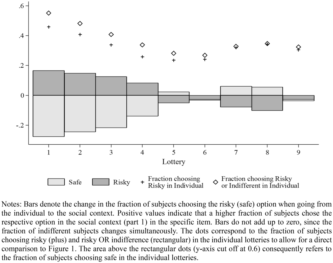
Fig. 2 Difference in choices between individual and social contexts

These differences are large in the unfavorable range. For T1 vs. T1i, T2 vs. T2i, T3 vs. T3i, and T4 vs. T4i, individuals take more risk when facing the social lottery than in the equivalent individual task, and the differences are highly significant (p < 0.01 for all four Stuart-Maxwell tests).Footnote ⁹ We observe for T1 to T4 that roughly 20% fewer subjects choose the safe option in the social context and about 10% more choose the risky one. The percentage of changes is relatively constant for all the unfavorable social situations. The fact that already a large share of subjects chooses the risky option for low probabilities in the individual task (T1i to T4i) partly masks the magnitude of the change from the individual to the social context. As an illustration, consider T1: While already only 45% of the subjects choose the safe lottery in the individual task (T1i), only 17% do so in the social context. Hence, in the social context 62% fewer subjects choose the safe option. The share of subjects moving away from the safe option in the social context ranges from 21 to 62% from T4(i) to T1(i). At the same time, the percentage increase in subjects choosing the risky option ranges from 32 to 36%. This is a substantial shift in choice patterns in the unfavorable domain.

The pattern is less clear for the favorable range. For T7 versus T7i and T8 versus T8i, there is more risk-taking in the individual tasks (p < 0.05 for Stuart-Maxwell tests). However, this result is not robust to using McNemar’s tests and pooling indifference with risky choices, since many subjects simply switch from the risky choice in the individual context to indifference in the social context. Other possible comparisons do not yield significant differences. Taking into account multiple hypotheses testing, one should not over-interpret the result.

Overall, we observe that decision-makers seem to be affected by the social context when making a risky decision, but not in a symmetric way. They unambiguously take more risk when the situation is unfavorable to them, but display similar choices when it is favorable to them compared to a risk-equivalent individual context.

This finding is robust to the different task ordering. Remember that we have sessions with the social context first and sessions with the individual context first. Generally, behavior in the individual and social lotteries is remarkably similar across the two orders. Mann–Whitney tests cannot reject equality of behavior between the two order treatments for any of the 18 lottery decisions.Footnote ¹⁰ Treatment effect patterns are (consequentially) similarly robust to the ordering.

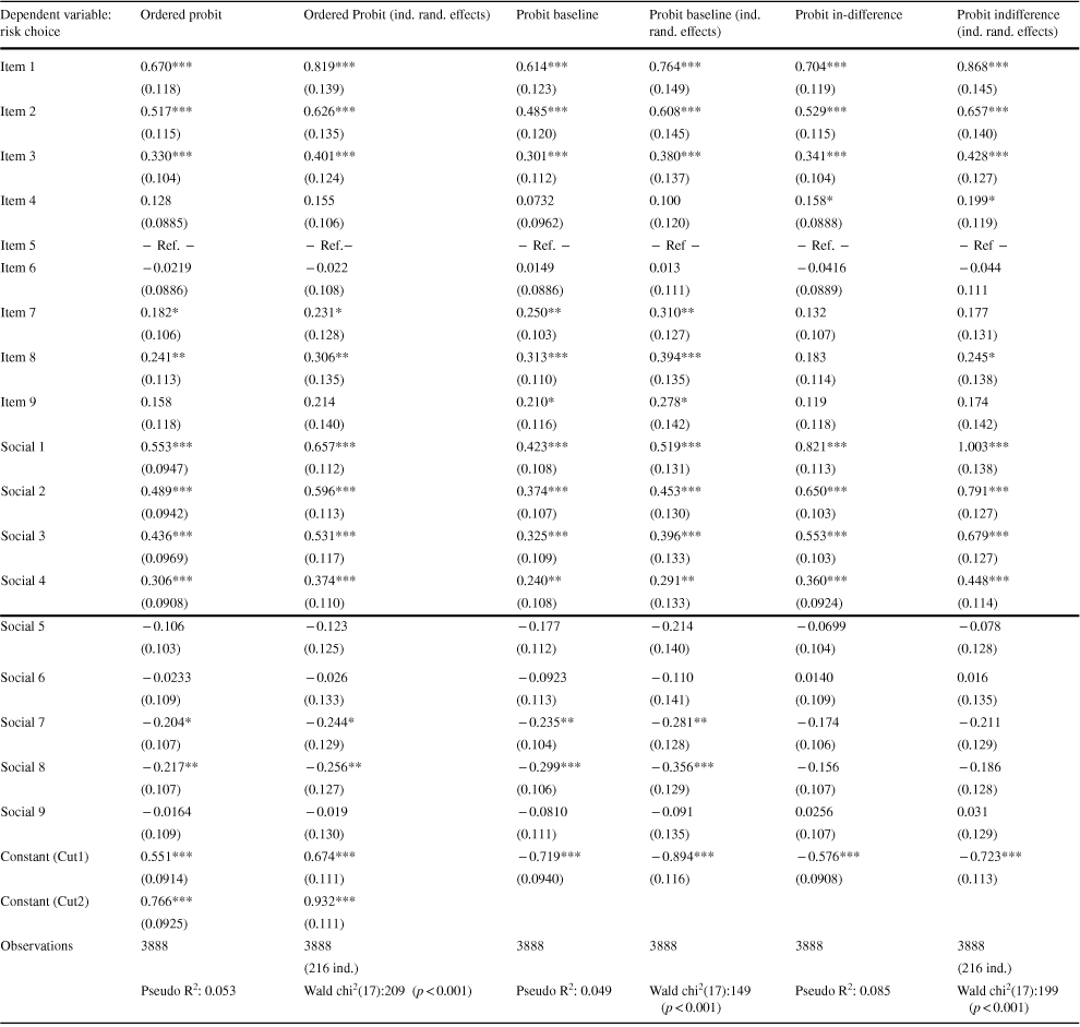
To further test the robustness of our results, we ran ordered probit models (columns 1 and 2 of Table 4) on the choices made in all 18 lotteries (with and without social context). We use indicator dummies for the nine categories of lotteries (Item 1 to Item 9) as defined by the probability of winning the prize for the decision-maker, without separating the social and individual tasks (Item 1 = 1 if p = 0.1, Item 2 = 1 if p = 0.2, etc.), and dummies Social 1, Social 2, etc. for the task being social (T1, … T9) or not (T1i, T9i). Hence, coefficients on Item 1 up to Item 9 correspond to the average risk-taking in the individual lottery tasks, while coefficients for Social 1, Social 2, etc. correspond to the additional risk-taking in the social context (relatively to the individual one). The results are displayed in Table 4,Footnote ¹¹ with column 1 corresponding to the pooled ordered probit estimation, while column 2 includes individual random effects.

Table 4 Risky choices in individual versus social context

Dependent variable: risk choice	Ordered probit	Ordered Probit (ind. rand. effects)	Probit baseline	Probit baseline (ind. rand. effects)	Probit in-difference	Probit indifference (ind. rand. effects)
Item 1	0.670***	0.819***	0.614***	0.764***	0.704***	0.868***
	(0.118)	(0.139)	(0.123)	(0.149)	(0.119)	(0.145)
Item 2	0.517***	0.626***	0.485***	0.608***	0.529***	0.657***
	(0.115)	(0.135)	(0.120)	(0.145)	(0.115)	(0.140)
Item 3	0.330***	0.401***	0.301***	0.380***	0.341***	0.428***
	(0.104)	(0.124)	(0.112)	(0.137)	(0.104)	(0.127)
Item 4	0.128	0.155	0.0732	0.100	0.158*	0.199*
	(0.0885)	(0.106)	(0.0962)	(0.120)	(0.0888)	(0.119)
Item 5	− Ref. −	− Ref.−	− Ref. −	− Ref −	− Ref. −	− Ref −
Item 6	− 0.0219	− 0.022	0.0149	0.013	− 0.0416	− 0.044
	(0.0886)	(0.108)	(0.0886)	(0.111)	(0.0889)	0.111
Item 7	0.182*	0.231*	0.250**	0.310**	0.132	0.177
	(0.106)	(0.128)	(0.103)	(0.127)	(0.107)	(0.131)
Item 8	0.241**	0.306**	0.313***	0.394***	0.183	0.245*
	(0.113)	(0.135)	(0.110)	(0.135)	(0.114)	(0.138)
Item 9	0.158	0.214	0.210*	0.278*	0.119	0.174
	(0.118)	(0.140)	(0.116)	(0.142)	(0.118)	(0.142)
Social 1	0.553***	0.657***	0.423***	0.519***	0.821***	1.003***
	(0.0947)	(0.112)	(0.108)	(0.131)	(0.113)	(0.138)
Social 2	0.489***	0.596***	0.374***	0.453***	0.650***	0.791***
	(0.0942)	(0.113)	(0.107)	(0.130)	(0.103)	(0.127)
Social 3	0.436***	0.531***	0.325***	0.396***	0.553***	0.679***
	(0.0969)	(0.117)	(0.109)	(0.133)	(0.103)	(0.127)
Social 4	0.306***	0.374***	0.240**	0.291**	0.360***	0.448***
	(0.0908)	(0.110)	(0.108)	(0.133)	(0.0924)	(0.114)
Social 5	− 0.106	− 0.123	− 0.177	− 0.214	− 0.0699	− 0.078
	(0.103)	(0.125)	(0.112)	(0.140)	(0.104)	(0.128)
Social 6	− 0.0233	− 0.026	− 0.0923	− 0.110	0.0140	0.016
	(0.109)	(0.133)	(0.113)	(0.141)	(0.109)	(0.135)
Social 7	− 0.204*	− 0.244*	− 0.235**	− 0.281**	− 0.174	− 0.211
	(0.107)	(0.129)	(0.104)	(0.128)	(0.106)	(0.129)
Social 8	− 0.217**	− 0.256**	− 0.299***	− 0.356***	− 0.156	− 0.186
	(0.107)	(0.127)	(0.106)	(0.129)	(0.107)	(0.128)
Social 9	− 0.0164	− 0.019	− 0.0810	− 0.091	0.0256	0.031
	(0.109)	(0.130)	(0.111)	(0.135)	(0.107)	(0.129)
Constant (Cut1)	0.551***	0.674***	− 0.719***	− 0.894***	− 0.576***	− 0.723***
	(0.0914)	(0.111)	(0.0940)	(0.116)	(0.0908)	(0.113)
Constant (Cut2)	0.766***	0.932***
	(0.0925)	(0.111)
Observations	3888	3888	3888	3888	3888	3888
		(216 ind.)				(216 ind.)
	Pseudo R²: 0.053	Wald chi²(17):209 (p < 0.001)	Pseudo R²: 0.049	Wald chi²(17):149 (p < 0.001)	Pseudo R²: 0.085	Wald chi²(17):199 (p < 0.001)

As dependent variable in columns 1 and 2 we use an ordinal scale for risk-taking (0 = safe choice, 1 = indifference, 2 = risky choice) for the relevant item. Columns 3 to 6 display results from regular probit regressions using an indicator variable for the choice being risky (column 3 and 4) and risky or indifferent (column 5 and 6). As independent variables we use dummies for all nine types of lotteries in general (Item 1 to 9), as well as nine indicator variables for the social context lotteries (Social 1 to 9). Hence, coefficients of the first nine dummies refer to risk-taking in the individual context, and the latter nine indicate whether for a given item, risk-taking is higher or lower in the social context. Standard errors are robust and clustered on the subject level

*p < 0.1, **p < 0.05, ***p < 0.01

Constant Cuts in columns 1 and 2 are threshold parameters of the ordered probit model to differentiate low risk takers from indifferent and risky subjects (Cut1) and low risk takers and indifferent subjects from risky subjects (Cut2). They are estimated such that Pr(Safe) = Pr(Xb + u < Cut1), Pr(Indifferent) = Pr(Cut1 < Xb + u < Cut2), and Pr(Risky) = Pr(Cut2 < Xb + u). Results are robust to using OLS or (ordered) logit.

The regression results confirm the findings based on non-parametric tests. Decision-makers indeed take more risk in unfavorable social situations compared to the equivalent individual situations. All terms indicating the social context are positive and significant in the unfavorable domain (at the 1%-level). For favorable situations, the effect is reversed. It seems like—if anything—individuals reduce risk-taking in the social context for favorable situations compared to situations without such context. These results are robust to using an ordinary probit model. Both when taking an indicator variable for risky choices only and when taking an indicator variable for risky and indifferent choices as dependent variables, we obtain the same pattern of results.

In sum, we observe some variability in the proportion of risky choices in the individual tasks, possibly related to a non-linear treatment of probabilities, but more relevantly for our research question at hand, we observe a strong effect of social comparisons in the unfavorable domain. In such tasks, participants take much more often the risky option than in the individual task. To the contrary, very little, if any, effect is found in the favorable domain.Footnote ¹²

Result 1

Decision-makers become relatively more risk-seeking in the unfavorable social domain compared to an equivalent individual decision-making task.

A side result is also that this difference observed in the unfavorable domain (in comparison to the equivalent individual decision-making task) does not seem to increase when getting closer to p = 0.5, as predicted by the discrete positional concern hypothesis. If anything, the difference increases as p get closer to 0 (0.553 for p = 0.1 versus 0.306 for p = 0.4).

Result 2

The behavior in the favorable social domain is not systematically different than in the individual decision-making task. If at all, there is a slight tendency of less risk-taking in the favorable social domain.

3.2 Individual heterogeneity

We now have a closer look at individual heterogeneity with three aims in mind. The first one is to check the robustness of our main findings when taking into account possible sampling variations in other characteristics (social preferences, risk attitudes, etc.). The second one is that these characteristics can be correlated with the strength of the effect we observe and shed some light on its psychological drivers. And the last one is to simply establish the heterogeneity of the sample with respect to the effect of social comparisons on risk-taking. For that purpose, we can look at the individual characteristics elicited in parts 2, 3 and 5 of our experiment. Table 5 provides an overview of these characteristics.

Table 5 Observables from parts 2, 3 and 5

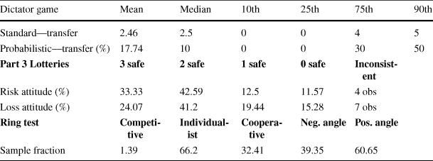
Dictator game	Mean	Median	10th	25th	75th	90th
Standard—transfer	2.46	2.5	0	0	4	5
Probabilistic—transfer (%)	17.74	10	0	0	30	50
Part 3 Lotteries	3 safe	2 safe	1 safe	0 safe	Inconsistent
Risk attitude (%)	33.33	42.59	12.5	11.57	4 obs
Loss attitude (%)	24.07	41.2	19.44	15.28	7 obs
Ring test	Competitive	Individualist	Cooperative	Neg. angle	Pos. angle
Sample fraction	1.39	66.2	32.41	39.35	60.65

One aspect in which subjects potentially differ is whether they are socially oriented, i.e. other-regarding (inequity averse, altruistic, etc.). Categorizing selfish and pro-social subjects on the basis of a median split in their offer in the dictator game in part 2 of the experiment provides us with additional insights.Footnote ¹³ Figure 3 shows the differences in choices for the two groups (for reasons of elucidation, call them “egoists” and “altruists”), when going from the individual to the social context.

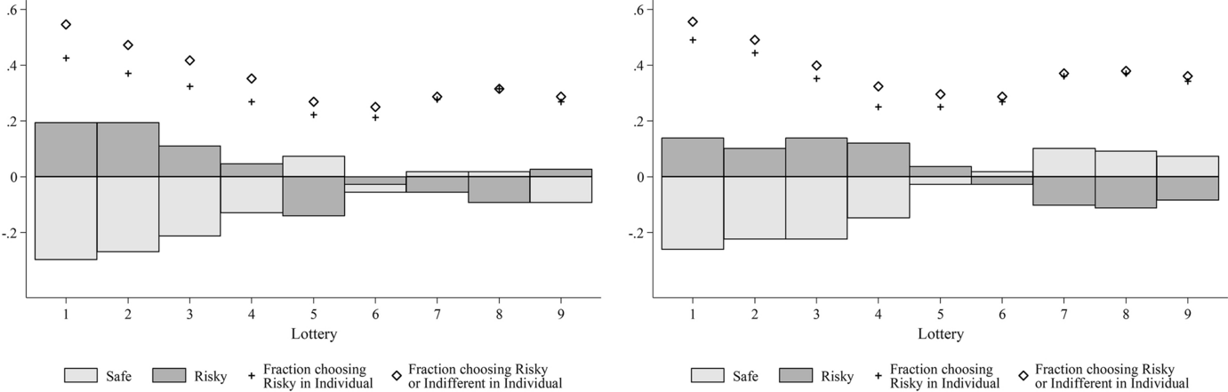
Fig. 3 Choices by dictator giving (left: egoists, right: altruists) in the social vs. individual context

For both groups, decision-making in the unfavorable range changes strongly from the individual to the social context. In the favorable range, slight differences between the groups emerge. Selfish participants switch from risky to safe from the individual to the social context. Altruists, however, show a less clear-cut pattern of change. They mainly switch to indifference, from both safe and risky choices in the individual context. These results remain roughly unchanged when we use generosity in the probabilistic dictator game for the sample split. They suggest that the observed effects of social comparisons are very widespread in the unfavorable domain, while in the favorable one, it may only concern self-interested participants, and to a much weaker extent even for them.

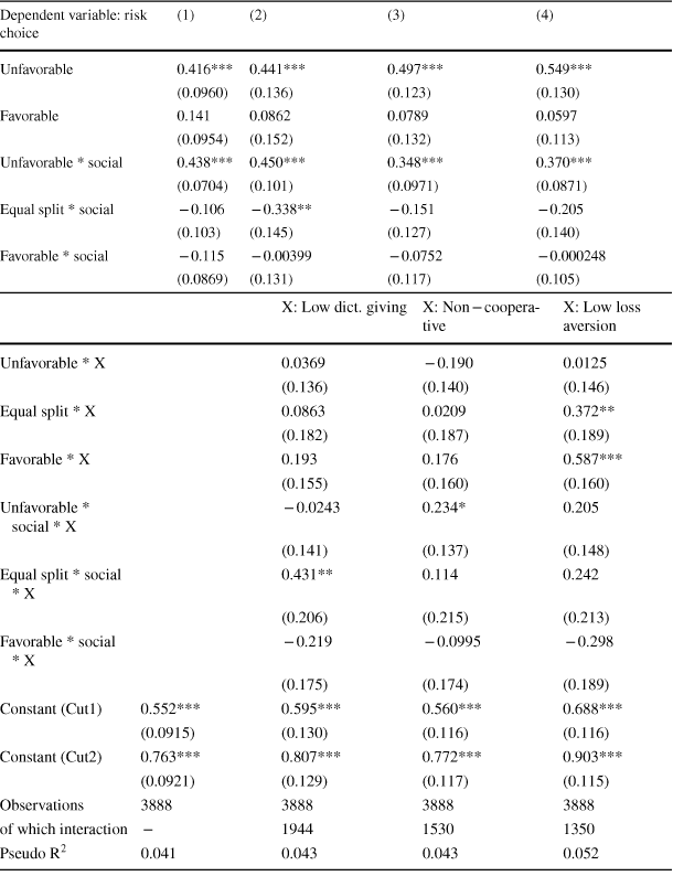
To see how these effects depend on other personal characteristics and to check their robustness, we ran ordered probit models similar to the ones in Table 4, including interaction terms with the different types of personal characteristics. For that purpose, in contrast to Table 4, we now only use three dummies for the different types of lotteries. This approach limits the number of interaction terms and makes the interpretation of the results more straightforward. Unfavorable is a dummy indicating that the lottery has an expected value below five [T1(i)–T4(i)]; Equal Split indicates the equal split lottery [T5(i)]; and Favorable stands for lotteries with an expected value for the decision-maker larger than 5 [T6(i)–T9(i)]. As before, we also include interaction terms for these lottery types with a dummy indicating the social context (Social). Column 1 shows results for this baseline specification with fewer dummy indicators than in Table 4. In columns 2–4, we interact the six baseline variables with an indicator variable for below-median dictator giving as in Fig.3 (column 2 of Table 6), for a negative angle in the ring test for social value orientation (column 3), and for low loss aversion (column 4) from part 3 of the experiment. This indicator variable is denoted X. A negative angle in the ring test implies that the decision-maker in part 5 of the experiment chose such that the matched participant received a negative payoff from these choices. This is only possible if, at least at one point for the 24 tasks, the decision-maker preferred to take money away from the matched participant, with no monetary benefit or possibly even at a cost to herself.Footnote ¹⁴ However, as argued above, being classified as individualistic with a negative angle already implies some form of competitive preferences. Low loss aversion (column 4) means that subjects at least in all but one of the loss aversion decisions chose the option involving the chance of a loss. This is true for 75 of our participants.

Table 6 Heterogeneity in the effects of the social context

Dependent variable: risk choice	(1)	(2)	(3)	(4)
Unfavorable	0.416***	0.441***	0.497***	0.549***
	(0.0960)	(0.136)	(0.123)	(0.130)
Favorable	0.141	0.0862	0.0789	0.0597
	(0.0954)	(0.152)	(0.132)	(0.113)
Unfavorable * social	0.438***	0.450***	0.348***	0.370***
	(0.0704)	(0.101)	(0.0971)	(0.0871)
Equal split * social	− 0.106	− 0.338**	− 0.151	− 0.205
	(0.103)	(0.145)	(0.127)	(0.140)
Favorable * social	− 0.115	− 0.00399	− 0.0752	− 0.000248
	(0.0869)	(0.131)	(0.117)	(0.105)

		X: Low dict. giving	X: Non − cooperative	X: Low loss aversion
Unfavorable * X		0.0369	− 0.190	0.0125
		(0.136)	(0.140)	(0.146)
Equal split * X		0.0863	0.0209	0.372**
		(0.182)	(0.187)	(0.189)
Favorable * X		0.193	0.176	0.587***
		(0.155)	(0.160)	(0.160)
Unfavorable * social * X		− 0.0243	0.234*	0.205
		(0.141)	(0.137)	(0.148)
Equal split * social * X		0.431**	0.114	0.242
		(0.206)	(0.215)	(0.213)
Favorable * social * X		− 0.219	− 0.0995	− 0.298
		(0.175)	(0.174)	(0.189)
Constant (Cut1)	0.552***	0.595***	0.560***	0.688***
	(0.0915)	(0.130)	(0.116)	(0.116)
Constant (Cut2)	0.763***	0.807***	0.772***	0.903***
	(0.0921)	(0.129)	(0.117)	(0.115)
Observations	3888	3888	3888	3888
of which interaction	−	1944	1530	1350
Pseudo R²	0.041	0.043	0.043	0.052

The dependent variable is an ordinal scale measure for risk-taking (as in Table 4). As in column 1 of Table 4, the columns report results from an ordered probit regression with robust and clustered standard errors

Grimm et al.p < 0.01, **p < 0.05, *p > 0.1

Constant Cuts are threshold parameters of the ordered probit model to differentiate low risk takers from indifferent and risky subjects (Cut1) and low risk takers and indifferent subjects from risky subjects (Cut2) (also see Table 4). Lottery types are now grouped in three blocks: Unfavorable [T1(i)–T4(i)], equal split [T5(i)], and favorable [T6(i)–T9(i)]. Columns (2)–(4) use different sample splits for the interaction terms. For each column, results in the upper part of the table (the first five lines) refer to risk-taking of subjects for whom X does not hold. For instance, for column 2, the first five lines correspond to coefficient estimates of the individuals who did not choose a low dictator gift. In contrast, the interaction terms of lines 6–11 refer to the effect of the social context on subjects for whom X holds, compared to the other subjects. More specifically, they describe whether risk-taking by subjects for whom X holds is different from that of subjects for whom X does not hold. For these lines, the first three coefficients refer to the difference in risk-taking in the individual context. The last three coefficients describe the difference in risk-taking in the social context for the subjects for whom X applies compared to the effect of the social context on subjects for whom X does not apply and by the effects of X applying in the individual context. A significant effect here indicates a relationship of the social context on subjects for whom X applies. The equal split is omitted for the individual context here. Results are robust to using OLS

Social value orientation, altruism and loss attitude do not seem to be related systematically to the sensitivity towards the social context, when it comes to decision-making under risk, at least for the measures used here.

The baseline regression results (column 1) again confirm the pattern already found for the finer-grained lottery definitions in Table 4. Compared to the individual context, average risk-taking increases for unfavorable tasks in the social context. If we now look at the regression results including interaction terms, interesting patterns emerge. For altruists—according to our dictator giving measure (upper part of column 2)—the increase in risk-taking due to the social context in unfavorable tasks is still positive and significant. The interaction term for unfavorable lotteries in the social context for selfish participants (Unfavorable * Social * X) is small and not significant. This also holds for other specifications of the altruism indicator: None of the differences in the social context between altruistic and selfish participants are statistically significant if we consider positive (non-zero) transfers as altruistic in both the standard and the probabilistic dictator game, or if we define above-median giving in the probabilistic dictator game as altruistic behavior. Overall, pro-sociality as measured by generosity in a Dictator Game does not seem to be related to the tendency to take more risk in unfavorable social contexts.

The differences appear somewhat larger for the split based on ring test choices (column 3 in Table 6). For less competitive types in the upper part of the table, as for altruists in column 2, choices in the unfavorable range are (weakly) affected by context. In this case, however, the more competitive types are more strongly affected by the social context (significant at the 10%-level only). Remember that the two measures for social preferences capture potentially different behavioral inclinations. Dictator giving is a proxy for altruism, whereas the ring test puts cooperative individuals against competitive individuals. The latter category cannot be captured by standard dictator giving decisions. It seems as if more competitive individuals show the strongest reaction to unfavorable situations in the social context.

Column 4 looks at interactions with loss attitude. Loss averse subjects, according to our measure, are, as in the overall pattern, affected by the social context in the unfavorable domain. Low loss-averse subjects seem, directionally, more strongly affected. The interaction term, however, is insignificant and also defining low loss aversion as choosing all three lotteries involving losses or as choosing only at least one lottery involving a potential loss does not lead to significant differences. Further, the coefficient on Unfavorable * Social * X is also insignificant if we consider indifference choices in the loss attitude task as taking the lottery involving the loss.

Result 3

Finally, we ran a k-medians clustering analysisFootnote ¹⁵ on all social lotteries, dividing the subjects into four clusters. This analysis resulted in the following characterization: the first and clearly largest class of decision-makers is comprised of 106 (out of 216) individuals who exhibit a strongly domain-dependent pattern of risk attitudes in the social context (strongly risk-seeking in the unfavorable situation, and risk-averse in the favorable situation); the second cluster (18 subjects) chooses indifference very often; the third cluster shows a similar difference in behavior when moving from the individual to the social context as the first type, but is overall less risk-taking (45 subjects); and the final cluster (47 individuals) displays increasing risk-taking for the favorable range as well as for extremely unfavorable items.Footnote ¹⁶ The results from the cluster analysis by types are shown in Fig.4.

Fig. 4 Choices by types (1–4) in the social vs. individual context. Notes: See Figs. 2 or 3 for an explanation of the bars and dots. The panels represent choices of type-1 to type-4 (from left to right) individuals from a cluster analysis

The categorization of subjects can help explain the aggregate pattern. The overall asymmetry in risky behavior across favorable and unfavorable situations seems to be mostly (but not only) driven by—the most prevalent—type-1 individuals. For these subjects, the increase in risk-taking in the unfavorable range when going from the individual to the social context is very pronounced, while they even reduce risk-taking in the favorable range. Type 2 individuals are most effectively characterized by their inclination towards indifference in the social lotteries, driving the overall observed increase in indifference in the social context.

Result 4

There is considerable heterogeneity in the sensitivity towards the social context, when it comes to decision-making under risk. About half of our participants react very strongly to the social context, both in the favorable domain (becoming relatively less risk-seeking) and in the unfavorable domain (becoming relatively more risk-seeking).

4 Discussion

Overall, our results suggest that individual attitudes towards risk are strongly affected by the social context. We observe systematic deviations in social situations from what decision-makers choose in similar situations under risk that do not allow for social comparisons. In the following, we deepen our discussion outlined in the introduction and the hypotheses section on potential explanations in the light of different utility functions or decision theories in turn.

A natural contender to explain a change in risk attitude in social situations is the role of (ex post) social preferences. Yet, it appears (see Prediction 3) that what matters is not so much the type of social preferences than the curvature (and a possible change of the type of curvature in different social domains) that may imply shifts in revealed risk attitude. Indeed, for various types of ex post social preferences it is easy to find a convex or concave version, that induces risk-seeking or risk-averse behavior. Hence, ex post social preferences can hardly explain the result we observe of more risk-taking in the unfavorable domain than in the absence of social comparisons. Likewise, ex ante (or “procedural” or “process”) fairness concerns cannot easily help in explaining our results (Trautmann Reference Trautmann2009; Trautmann and Wakker Reference Trautmann and Wakker2010). Ex ante, both options provide the same expected payoff to both participants. Consequently, procedural inequity aversion preferences should not affect individual choices unless the decision-maker has a preference for a stochastic allocation decision over a deterministic one. For instance, one could feel less responsibility for the stochastically implemented uneven distribution than for one that is implemented deterministically. Notice, however, that our subjects had the possibility to indicate indifference and let a random mechanism decide. Part of the strong increase in indifferent choices that we observe could be related to this, but that makes responsibility avoidance less of a plausible candidate for favoring the risky option.

Overall our data pattern is consistent with three explanations based on (i) gloating (Prediction 4), (ii) positional concerns (Prediction 5), and (iii) a social reference point (Prediction 6).

Regarding the first explanation, the hypothesis that gloating looms larger than envy predicts—in the simplified case of a piecewise linear utility—that decision-makers will take risks, when the probability of winning is less than or equal to 0.5 and will go for the safe option otherwise. This fits roughly our data. Yet, one specific prediction is at odds with what we experimentally observe. For the specific case of p = 0.5, subjects overwhelmingly choose the safe option. Even more importantly, p = 0.5 is the social lottery task for which subjects choose the risky option least often, in contrast to what is predicted by the “gloating” hypothesis.

Regarding the second explanation, that is positional considerations generate a discrete utility bonus (in case of being ahead) or a discrete utility penalty (in case of being behind), we observe that, generally speaking, it fits our data, with people going for the risky option in the unfavorable domain, yet being satisfied with the safe option in the favorable one. The behavior in p = 0.5 is not conclusive, as for the gloating hypothesis, the behavior of decision-makers for equal positions is left undetermined in the model.Footnote ¹⁷ Yet, as stated in Sect. 3.1, the positional concerns imply that their effect on risk-taking (more risk-taking in the unfavorable domain, less in the favorable domain) should be all the stronger the closer the probability is to 0.5. Put differently, we should hardly observe any effect for T1, where p = 0.1, and observe a strong effect for T4, where p = 0.4. This is clearly the opposite of what we find. Although in theory compatible with the general results, details of the data make it unlikely that positional concerns explain our results.

The third explanation is the idea that the other’s payoff could play the role of a reference point in prospect theory, an idea developed by Linde and Sonnemans (Reference Linde and Sonnemans2012). Consequently, gain and loss domains would be defined through the earnings of the other participant, predicting more risk-seeking in the loss domain (unfavorable situations) and more risk-aversion in the gain domain (favorable situations). When in favorable situations, subjects in our experiment could mainly lose relative to the other participant when choosing the risky option. Instead, by selecting the safe option they can secure their relative social gain. In contrast to that, in unfavorable situations, subjects are not much affected by the prospect of getting (0,10) rather than (1,9) because of diminishing sensitivity (i.e. convex utility) in the (relative) loss domain. Gambling in this case means a large probability of a subjectively small loss but a small probability of a very large gain. Such reasoning could also help to explain the data by Haisley et al. (Reference Haisley, Mostafa and Loewenstein2008) who show that, when reminded of their low status, low income individuals were more likely to engage in risky purchases such as buying lottery tickets. It is also the reasoning of Schwerter (Reference Schwerter2013), indicating that decision-makers indeed experience social losses and gains in a risk task when exposed to another participant receiving a varying fixed payment. The social reference point hypothesis hence corresponds quite well with the change of risk attitudes we observe between “social gains” and”social losses”, or the favorable domain and the unfavorable domain. In contrast to the two alternative hypotheses, the social reference point hypothesis has no particular implication for the size of the effect when p varies between 0.1 and 0.4, and more relevantly, does predict a strong aversion to risk at p = 0.5 (because of ‘relative’ loss aversion, and not because of the change of curvature, as generically put forth in Rabin Reference Rabin2000).

Our findings concerning individual heterogeneity are in line with arguments in favor of a social reference point. Those decision-makers that reduce the other’s payoff in the ring test—if anything—exhibit the overall pattern more strongly than those that do not. Reducing the other’s payoff can only be rationalized by making some form of relative comparisons with the matched participant and by a wish to earn more in relative terms (apart from pure forms of anti-social behavior). It is not surprising that these individuals are more strongly affected by social comparisons. The cluster analysis also helps rationalizing the patterns. Type-1 individuals, who drive the aggregate pattern described above, are not only disproportionally less often categorized as cooperative, they also explicitly state motivations based on a social reference point story. In the subjects’ comment section at the end of the experiment, where participants were supposed to elaborate on their motivation behind choices in the social context task, one type-1 subject explained switching to the risky option in the unfavorable cases by stating that “as long as I earned more than the other, I chose the certain amount”. Another explicitly wanted to “get a higher payoff than the other”. These statements are a specific characteristic of type-1 individuals.

In contrast to the large group of type-1 individuals, there seems to be something else driving behavior of type-2 and type-4 decision-makers. Responsibility aversion is one potential explanation. Type-2 individuals are characterized by a switch towards indifference in unfavorable tasks in the social context—and slightly less pronounced in the favorable context. This might in part be driven by responsibility avoidance, which could have also led to the results in Kircher et al. (Reference Kircher, Ludwig and Sandroni2013). Subjects’ comments provide some indication for such a conclusion. One subject, for example, explicitly stated that she did not want to make the decision herself, but rather leave it to luck.Footnote ¹⁸ Similar mechanisms could apply to type-4 subjects. Choosing the risky option more often in favorable social decisions implies that, in the end, it is the random draw that establishes an uneven distribution and not the participant’s choice. Procedural fairness concerns are another potential explanation for type-4 subjects. Even though procedural concerns (Trautmann Reference Trautmann2009; Bolton et al. Reference Bolton, Brandts and Ockenfels2005; SaitoReference Saito2013) should play no role with equivalent expected outcomes for both options, it might still be that a subset of individuals perceives the risky lottery to be fairer in the favorable range. Giving a chance (even if small) to get the entire amount could be considered as more appropriate than implementing for sure a very unequal payoff structure. Some participants’ comments are consistent with both lines of reasoning. One subject explicitly stated that he or she chose out of fairness concerns and another said that probabilistic decisions reduce the responsibility and feeling of guilt.

5 Conclusion

Our data suggest that risk-taking is influenced by the relative social situation of the decision-maker. Compared to equivalent situations without a social context, more risk is chosen in unfavorable situations, while similar risk-taking is observed for favorable social situations. A large share of our decision-makers exhibits this pattern in a pronounced way.

This observed behavioral pattern cannot be straightforwardly explained by extensions of models of outcome-based social preferences for stochastic environments based on expected utility theory. The overall asymmetric pattern rather points towards the importance of social reference points. Future experiments should try to assesses the robustness of this conclusion, in particular with respect to alternative explanations that are in line with the general pattern, but fail on the details of the observed behavior in our setup (positional concerns, gloating being stronger than envy). This is especially important as experimental results in the relevant literature are not all fully consistent in their results.

Our experimental results suggest that the role of social context may be critical also in understanding organizational and financial risk-taking. When subjects directly compete against each other (e.g., over resources or power), even without any explicit competition incentives such as tournament prizes, they might take excessive risks that they would not take absent information on outcomes of others. Information provision or the way this information is presented may affect managers and investors alike.

In a broader context, our study provides another piece of evidence for the idea that risk-taking is strongly affected by the social environment in which decisions take place. Future studies could test specific theoretical models of excessive risk-taking that embed the risky situation into a social environment. Further, the social situation could be varied in different dimensions (such as the level of competition, the size of the references group, the presentation of information, etc.), not only along the outcome dimension.

Funding

Open access funding provided by University of Vienna. Financial support by the LMU Munich is gratefully acknowledged. Grimm and Kocher acknowledge financial support by the German Research Foundation (DFG) through GRK 1928 and through CRC TRR 190.

Footnotes

Electronic supplementary material The online version of this article (https://doi.org/10.1007/s10683-020-09690-8) contains supplementary material, which is available to authorized users.

¹ These effects include peer effects, where the choice of a third party has an impact on the choice of the decision-maker (e.g., Cooper and Rege Reference Cooper and Rege2011; Bursztyn et al. Reference Bursztyn, Ederer, Ferman and Yuchtman2014; Cai et al. Reference Cai, de Janry and Sadoulet2015; Lahno and Serra-Garcia Reference Lahno and Serra-Garcia2015), social preferences, for which the distribution of risks may be a component of ex-ante fairness or benevolence (Brennan et al. Reference Brennan, Güth, Gonzalez and Levati2008; Krawczyk and Le Lec Reference Krawczyk and Le Lec2010; Brock et al. Reference Brock, Lange and Ozbay2013), more generally the fact to be (at least in part) responsible for another individual’s financial situation (e.g., Bolton et al. Reference Bolton, Ockenfels and Stauf2015; Chakravarty et al. Reference Chakravarty, Harrison, Haruvy and Rutström2011; Vieider et al. Reference Vieider, Villegas-Palacio, Martinsson and Mejía2015), and the correlation between the decision-maker and the third party’s fortune (Adam et al. Reference Adam, Kroll and Teubner2014; Friedl et al. Reference Friedl, de Miranda and Schmidt2014, albeit not replicated by Krawczyk et al. Reference Krawczyk, Trautmann and van de Kuilen2017). Another systematic approach is to study the correlation of risk attitudes and social preferences at the individual level (e.g., Müller and Rau Reference Müller and Rau2016).

² Fafchamps et al. (Reference Fafchamps, Kebede and Zizzo2015) and Dijk et al. (Reference Dijk, Holmen and Kirchler2014) also find that investors on experimental asset markets performing below the average favor positively skewed portfolios (those that have a small chance for very high returns), while those performing above the average prefer negatively skewed portfolios. The effects occur independently of whether others’ outcomes are payoff-relevant (in the form of tournament-based incentives) or not.

³ We partly had a more informal discussion of theoretical considerations in the original version of our paper, and we thank the reviewers for pointing out some of the important aspects discussed in the following.

⁴ More details for Sects. 2.2.3 and 2.2.4 are provide in Online Appendix D.

⁵ The other plausible case does not raise much interest: if α M , 1 - α M ≻ M , 0 ≻ 0 , M , then the decision-maker will choose α M , 1 - α M in all circumstances, that is, the decision-maker will prefer the certain combination over the probabilistic one.

⁶ To illustrate that social risk attitude is not (only) determined by the type of social preferences, consider the following examples: the decision-maker can be altruistic with a concave utility (for instance, u x 1 , x 2 = x 1 a + b x 2 y a with a < 1 and b ∈ 0 , 1 ), altruistic with a convex utility (for instance, u x 1 , x 2 = x 1 a + b x 2 a with a > 1 and b ∈ 0 , 1 ), spiteful/rival with a concave utility (for instance u x 1 , x 2 = x 1 a + b x 2 c with a < 1 , b ∈ - 1 , 0 , c > 1 ), spiteful/rival with a convex utility (for instance, u x 1 , x 2 = x 1 a + b x 2 c with a > 1 , b ∈ - 1 , 0 , c < 1 ), etc. The general nature of (ex post) social preferences (pro-social or anti-social) have little to do with social risk attitudes per se.

⁷ We cannot exclude that the truncation has some behavioral effects on choices.

⁸ With very few exceptions, only LMU Munich students join the MELESSA subject pool. Since there is more than one university at Munich, some participants may come from other universities. Many of them remain in the pool after graduation (with no requirement to update their status), but most of the graduates rarely take part in experiments, and inactive subject pool members are deleted from the subject pool data base approximately once a year. Given that 75% of our subjects were 26 or younger, we can safely say they were mostly students but we cannot provide an exact number. It is the policy of the laboratory not to record too many privacy details of participants.

⁹ If we pool indifference and safe option choices, McNemar’s tests of marginal homogeneity result in differences that are significant at the 1%-level for T1 vs. T1i, T2 vs. T2i, and T3 vs. T3i, and significant at the 5%-level for T4 vs. T4i. If we pool indifference with risky choices, all tests are significant at the 1%-level.

¹⁰ Power to detect effects is not a concern here. With 144 subjects in the order as described in the design section and 72 subjects in the reverse order, we get a moderate required effect size of 0.4 for a beta of 0.8 and alpha of 0.05.

¹¹ Our findings from Tables 4 and 6 (see below) are fully robust to using linear (probability) models or logistic specifications. This also addresses concerns regarding the interpretation of interaction terms in non-linear models (Ai and Norton Reference Ai and Norton2003; Greene Reference Greene2010). Further, inference based on manually calculated correct marginal effects does not yield different insights compared to the coefficients reported in Tables 4 and 6. To the best of our knowledge, methods for statistical power calculations are less obvious for the probit models that we use. For OLS approximations, our sample size is large enough to detect quite small effect sizes.

¹² We have run a pilot classroom experiment that was mentioned in earlier versions of this paper. All of our main results show up there as well, despite a smaller sample size, a smaller expected stake size and somewhat less control. The results of this classroom experiment are described in Appendix E.

¹³ Exactly 50% of the dictators give nothing, €1, or €2.

¹⁴ In our preferred specification, we refrain from using the strict classification into types (individualistic, competitive, cooperative, etc.) described in Appendix A, since we only have two subjects classified as purely competitive and a vast majority in the individualistic category.

¹⁵ The K-medians clustering partitions subjects into k groups by finding k centroids that minimize the overall distance between data points and the closest centroid. Four clusters are chosen, since the reduction in the within (cluster) sum of squares is large until the addition of the fourth cluster, but gets very small for larger numbers of clusters. The use of medians rather than means (“k-means clustering”) is more appropriate for discrete data, as is the case here.

¹⁶ The exact clustering always depends on the random starting points for building the clusters. Hence, if we had randomly selected different starting points, we would have ended up with slightly different clusters.

¹⁷ Indeed, winning can include draws (or not). This gives some degrees of freedom in the model that can be used to predict a safe choice for the equal situation.

¹⁸ It also seems that these subjects are genuinely more altruistic. In both the deterministic and the probabilistic dictator game, on average, they give the most to recipients.

Springer Nature remains neutral with regard to jurisdictional claims in published maps and institutional affiliations.

References

Adam, MT, Kroll, EB, & Teubner, T (2014). A note on coupled lotteries. Economics Letters, 124(1), 96–99.CrossRef Google Scholar

Ai, C, & Norton, EC (2003). Interaction terms in logit and probit models. Economics Letters, 80(1), 123–129.CrossRef Google Scholar

Bault, N, Coricelli, G, & Rustichini, A (2008). Interdependent utilities: How social ranking affects choice behavior. PLoS ONE, 3(10), e3477.CrossRef Google Scholar PubMed

Bolton, G, & Ockenfels, A (2010). Betrayal Aversion: Evidence from Brazil, China, Oman, Switzerland, Turkey, and the United States: Comment. American Economic Review, 100(1), 628–633.CrossRef Google Scholar

Bolton, GE, Brandts, J, & Ockenfels, A (2005). Fair procedures: evidence from games involving lotteries. Economic Journal, 115(506), 1054–1076.CrossRef Google Scholar

Bolton, GE, Ockenfels, A, & Stauf, J (2015). Social responsibility promotes conservative risk behavior. European Economic Review, 74, 109–127.CrossRef Google Scholar

Bolton, GE, Zwick, R, & Katok, E (1998). Dictator game giving: rules of fairness versus acts of kindness. International Journal of Game Theory, 27(2), 269–299.CrossRef Google Scholar

Brock, M, Lange, A, & Ozbay, EY (2013). Dictating the risk–Experimental evidence on giving in risky environments. American Economic Review, 103(1), 415–437.CrossRef Google Scholar

Brandts, J, & Charness, G (2011). The strategy versus the direct-response method: a first survey of experimental comparisons. Experimental Economics, 14(3), 375–398.CrossRef Google Scholar

Brennan, G, Güth, W, Gonzalez, L, & Levati, MV (2008). Attitudes toward private and collective risks in individual and strategic choice situations. Journal of Economic Behavior and Organization, 67(1), 253–262.CrossRef Google Scholar

Brosig, J (2002). Identifying cooperative behavior: Some experimental results in a prisoner’s dilemma game. Journal of Economic Behavior and Organization, 47(3), 275–290.CrossRef Google Scholar

Bursztyn, L, Ederer, F, Ferman, B, & Yuchtman, N (2014). Understanding mechanisms underlying peer effects: Evidence from a field experiment on financial decisions. Econometrica, 82(4), 1273–1301.Google Scholar

Cai, J, de Janry, A, & Sadoulet, E (2015). Social networks and the decision to insure. American Economic Journal: Applied Economics, 7(2), 81–108.Google Scholar

Chakravarty, S, Harrison, GW, Haruvy, EE, & Rutström, EE (2011). Are you risk-averse over other people's money?. Southern Economic Journal, 77(4), 901–913.CrossRef Google Scholar

Charness, G, Masclet, D, & Villeval, MC (2013). The dark side of competition for status. Management Science, 60(1), 38–55.CrossRef Google Scholar

Cooper, D, & Rege, M (2011). Misery loves company: Social regret and social interaction effects in choices under risk and uncertainty. Games and Economic Behavior, 73(1), 91–110.CrossRef Google Scholar

Dijk, O, Holmen, M, & Kirchler, M (2014). Rank matters – The impact of social competition on portfolio choice. European Economic Review, 66, 97–110.CrossRef Google Scholar

Fafchamps, M, Kebede, B, & Zizzo, DJ (2015). Keep up with the winners: Experimental evidence on risk-taking, asset integration, and peer effects. European Economic Review, 79, 59–79.CrossRef Google Scholar

Fischbacher, U (2007). z-Tree: Zurich Toolbox for ready-made Eeonomic experiments. Experimental Economics, 10(2), 171–178.CrossRef Google Scholar

Forsythe, R, Horowitz, J, Savin, N, & Sefton, M (1994). Fairness in simple bargaining experiments. Games and Economic behavior, 6(3), 347–369.CrossRef Google Scholar

Friedl, A, de Miranda, KL, & Schmidt, U (2014). Insurance demand and social comparison: An experimental analysis. Journal of Risk and Uncertainty, 48(2), 97–109.CrossRef Google Scholar

Gamba, A, Manzoni, E, & Stanca, L (2017). Social comparison and risk-taking behavior. Theory and Decision, 82(2), 221–248.CrossRef Google Scholar

Greene, W (2010). Testing hypotheses about interaction terms in nonlinear models. Economics Letters, 107(2), 291–296.CrossRef Google Scholar

Greiner, B (2015). Subject pool recruitment procedures: Organizing experiments with ORSEE. Journal of the Economic Science Association, 1(1), 114–125.CrossRef Google Scholar

Haisley, E, Mostafa, R, & Loewenstein, G (2008). Subjective relative income and lottery ticket purchases. Journal of Behavioral Decision-making, 21(3), 283–295.CrossRef Google Scholar

Herstein, IN, & Milnor, J (1953). An axiomatic approach to measurable utility. Econometrica, 21(2), 291–297.CrossRef Google Scholar

Holt, C, & Laury, S (2002). Risk aversion and incentive effects. American Economic Review, 92(5), 1644–1655.CrossRef Google Scholar

Kahneman, D, & Tversky, A (1979). Prospect theory: An analysis of decision under risk. Econometrica, 47(2), 263–291.CrossRef Google Scholar

Kircher, P, Ludwig, S, & Sandroni, A (2013). On the difference between social and private goods. The BE Journal of Theoretical Economics, 13(1), 155–177.Google Scholar

Krawczyk, M, & Le Lec, F (2010). ’Give me a chance!’ An experiment in social decision under risk. Experimental Economics, 13(4), 500–511.CrossRef Google Scholar

Krawczyk, MW, Trautmann, ST, & van de Kuilen, G (2017). Catastrophic risk: Understanding insurance decisions. Theory and Decision, 82(3), 309–326.CrossRef Google Scholar

Kuziemko, I, Buell, RW, Reich, T, & Norton, MI (2014). ‘Last-place aversion’: Evidence and redistributive implications. Quarterly Journal of Economics, 129(1), 105–149.CrossRef Google Scholar

Lahno, AM, & Serra-Garcia, M (2015). Peer effects in risk-taking: Envy or conformity?. Journal of Risk and Uncertainty, 50(1), 75–93.CrossRef Google Scholar

Linde, J, & Sonnemans, J (2012). Social comparisons and risky choices. Journal of Risk and Uncertainty, 44(1), 45–72.CrossRef Google Scholar

Müller, S, & Rau, HA (2016). The relation of risk attitudes and other-regarding preferences: A within-subjects analysis. European Economic Review, 85(1), 1–7.CrossRef Google Scholar

Offerman, T, Sonnemans, J, & Schram, A (1996). Value orientations, expectations and voluntary contributions in public goods. Economic Journal, 106(437), 817–845.CrossRef Google Scholar

Rabin, M (2000). Risk aversion and expected-utility theory: A calibration theorem. Econometrica, 68(5), 1281–1292.CrossRef Google Scholar

Saito, K (2013). Social preferences under risk: Equality of opportunity versus equality of outcome. American Economic Review, 103(7), 3084–3101.CrossRef Google Scholar

Selten, R, & Sauermann, H (1967). Die Strategiemethode zur Erforschung des eingeschränkt rationalen Verhaltens im Rahmen eines Oligopolexperiments. Beiträge zur experimentellen Wirtschaftsforschung, Tübingen: Mohr 136–168.Google Scholar

Schwerter, F. (2013). Social reference points and risk-taking, Bonn Econ Discussion Papers, 11/2013.Google Scholar

Trautmann, S (2009). A tractable model of process fairness under risk. Journal of Economic Psychology, 30(5), 803–813.CrossRef Google Scholar

Trautmann, ST, Vieider, FM Roeser, S, Hillerbrand, R, Sand, P, & Peterson, M (2012). Social influences on risk attitudes: Applications in economics. Handbook of risk theory Epistemology, decision theory, ethics, and social implications of risk, Amsterdam: Springer 575–600.CrossRef Google Scholar

Trautmann, ST, & Wakker, P (2010). Process fairness and dynamic consistency. Economics Letters, 109(3), 187–189.CrossRef Google Scholar

Tversky, A, & Kahneman, D (1992). Advances in prospect theory: Cumulative representation of uncertainty. Journal of Risk and Uncertainty, 5(4), 297–323.CrossRef Google Scholar

Van Dijk, F, Sonnemans, J, & van Winden, F (2002). Social ties in a public good experiment. Journal of Public Economics, 85(2), 275–299.CrossRef Google Scholar

Van Lange, P, De Bruin, E, Otten, W, & Joireman, JA (1997). Development of prosocial, individualistic, and competitive orientations: Theory and preliminary evidence. Journal of Personality and Social Psychology, 73(4), 733–746.CrossRef Google Scholar PubMed

Vieider, F, Villegas-Palacio, C, Martinsson, P, & Mejía, M (2015). Risk-taking for oneself and others: A structural model approach. Economic Inquiry, 54(2), 879–894.CrossRef Google Scholar

Wakker, P (2010). Prospect theory: For risk and ambiguity, Cambridge: Cambridge University Press.CrossRef Google Scholar

Table 1 Part 1—social context tasks

Table 2 Part 4—individual context tasks

Table 3 Part 3—risk and loss attitude choices

Fig. 1 Distribution of choices in the social context

Fig. 2 Difference in choices between individual and social contexts

Table 4 Risky choices in individual versus social context

Table 5 Observables from parts 2, 3 and 5

Fig. 3 Choices by dictator giving (left: egoists, right: altruists) in the social vs. individual context

Table 6 Heterogeneity in the effects of the social context

Fig. 4 Choices by types (1–4) in the social vs. individual context. Notes: See Figs. 2 or 3 for an explanation of the bars and dots. The panels represent choices of type-1 to type-4 (from left to right) individuals from a cluster analysis

Grimm et al. supplementary material

Online Appendix: Sharing or gambling? On risk attitudes in social contexts

File 111.3 KB

Article contents

Sharing or gambling? On risk attitudes in social contexts

Abstract

Keywords

JEL classification

1 Introduction

2 Experimental design and procedures

2.1 Decision-making under risk in varying decision contexts

2.2 Theoretical considerations

2.2.1 Self-interested expected utility maximizers

Prediction 1

Prediction 2

2.2.2 Definition of social risk attitude

Definition 1

2.2.3 Social risk attitude and (ex post) social preferencesFootnote 4

Prediction 3

2.2.4 Changes in social risk attitudes

Prediction 4

Prediction 5

Prediction 6

2.3 Experimental controls

2.4 Experimental procedures

3 Experimental results

3.1 Aggregate results

Result 1

Result 2

3.2 Individual heterogeneity

Result 3

Result 4

4 Discussion

5 Conclusion

Funding

Footnotes

References

Grimm et al. supplementary material

Save article to Kindle

Save article to Dropbox

Save article to Google Drive

Reply to: Submit a response

Your details

You have entered the maximum number of contributors

Conflicting interests

2.2.3 Social risk attitude and (ex post) social preferencesFootnote ⁴