1 Introduction

A growing body of literature has highlighted the low, and somewhat unpredictable uptake of preventive technologies (Dupas Reference Dupas2011). In the United States, uptake of sunscreen (Holman et al. Reference Holman, Berkowitz, Guy, Hawkins, Saraiya and Watson2015) and tooth brushing (American Dental Association Reference Association2010) remains far from universal. Despite substantial evidence that physical exercise can forestall numerous non-communicable and chronic diseases, nearly 40% of individuals in high-income countries report engaging in insufficient physical activity (Guthold et al. Reference Guthold, Stevens, Riley and Bull2018). While there have been a number of advances in technologies that screen for colorectal cancer, screening for colorectal cancer remains low (Daskalakis et al. Reference Daskalakis, DiCarlo, Hegarty, Gudur, Vernon and Myers2020). Other evidence suggests that adherence to statins prescribed as primary prevention for heart disease is also sub-optimal, with non-adherence to regular pill taking observed for more than half of individuals prescribed a statin within just 1 year (Ofori-Asenso et al. Reference Ofori-Asenso, Jakhu, Zomer, Curtis, Korhonen and Nelson2018).

Individuals choosing to experiment with health prevention technologies (whether it be a drug or lifestyle change such as increased physical activity) may update their priors based on their experiences. Preventive health investments do not eliminate the chance of adverse events, but rather reduce the likelihood of adverse outcomes from a given baseline risk to a smaller non-zero probability. The specific risk reduction offered by preventative health technologies are unlikely to be known by users, and are not typically provided as part of public health campaigns in practice. Therefore, individuals may use their own experience and the experience of others to learn about the costs and benefits of investing in preventive health technologies.

Learning, however, cannot fully rationalize all behavior patterns observed in the empirical literature on preventive health investment. Learning about risk and effectiveness should decrease with age, which has not been found in the literature (Jin and Koch Reference Jin and Koch2018). If updating of priors was the primary mechanism, we should also see similar impacts for information campaigns and disease outbreaks, which is generally not the case (Oster Reference Oster2018), and we would not expect to see very large responses to temporary shocks (Jin and Koch Reference Jin and Koch2018; Oster Reference Oster2018).

In this paper, we develop a formal learning model of prevention to describe the conditions under which expected-utility-maximizing Bayesian learners take up prevention with unknown protective effects but known costs. We show that only those agents whose prior on a preventive health technology’s effectiveness exceeds a certain threshold will prevent, and that for any initial distribution of priors, preventive uptake will likely decline over time. We also show that in higher risk environments, agents respond less strongly to the failure of a preventive measure.

We then test the predictions of this model through a series of incentivized decision experiments in the lab. In our experiment, subjects were fully informed about the risk of getting sick without prevention and introduced to a range of preventive health technologies that lowered their probability of falling sick and losing their income in each period. After each adoption decision, health outcomes were stochastically determined as a function of the chosen strategy, and subjects were informed about their health outcome and resulting income.

In order to observe the impact of subjective experiences on uptake in different environments, we randomly assigned subjects to different levels of technology effectiveness and different levels of baseline risk. We also randomly assigned subjects to receive public health messages encouraging adoption. We hypothesized that these messages would lead to increased expectations about the effectiveness of the technology and encourage prevention initially, but this effect would fade over time as subjects updated their priors to more accurately reflect the true effectiveness of the technology.

Consistent with prevention patterns observed empirically in various settings (Dupas Reference Dupas2011) we find that a substantial fraction of subjects (20–40%) do not take up prevention. We also find that average prevention rates decline over time and that subjects with negative preventive outcomes revise their effectiveness prior downwards. Revisions of priors are weaker in higher risk environments where failures are expected to happen more frequently. The declining willingness to invest into prevention (as a private good) over time is similar to recent experimental evidence on behavior in public goods provision (Burton-Chellew et al. Reference Burton-Chellew, Nax and West2015).

Messages encouraging adoption have a small positive effect, increasing prevention by about 10%. This effect is stronger with the first technology subjects get exposed to but dissipates once a new technology is introduced.

We also see evidence of behaviors that are less consistent with rational learning models. Experimental subjects react more strongly to their most recent experiences than to experiences in the past, and tend to immediately switch out of prevention if they experience a negative outcome, even if they had multiple successful rounds before.

This immediate “reactivity” is even more obvious when it comes to behavioral responses to outcomes that do not reveal any information. Specifically, a rational learning model would predict no updating from stochastic health outcomes experienced when not using the prevention technology. However, we find that subjects who chose not to prevent are much more likely to switch to prevention in the following round after a negative health outcome than after a positive health outcome. Given that subjects were perfectly informed about the risks of adverse events without prevention, this suggests that some of the observed switching is the result of a behavioral response (“reacting”) to undesired outcomes rather than learning.

The results presented in this paper contribute to a growing literature on the role of learning and learning algorithms in understanding the adoption of new technologies more generally. An extensive experimental economics literature has focused on understanding learning processes over repeated decisions (see Erev and Haruvy (Reference Erev, Haruvy, Kagel and Roth2016) for an overview). In the context of agriculture, several studies suggest that levels of experimentation with new technologies are inefficiently low (Conley and Udry Reference Conley and Udry2010; Foster and Rosenzweig Reference Foster and Rosenzweig1995). The results of this study suggest that low initial uptake should be expected in settings where priors are diffuse and agents are risk-averse. Our model also predicts that uptake of technologies will likely decline rapidly over time in settings where poor outcomes with the technology are common due to random external events such as rainfall or pest.

Several explanations for low adoption have been proposed in the literature, including lack of information, high (effort) cost associated with learning (Chassang et al. Reference Chassang, Padró i Miquel and Snowberg2012), aversion to risk (Anderson and Mellor Reference Anderson and Mellor2009), aversion to ambiguity (Bryan Reference Bryan2010; Engle-Warnick et al. Reference Engle-Warnick, Escobal and Laszlo2007), problems with self-control (Dupas Reference Dupas2011), disagreements at the household level (Ashraf et al. Reference Ashraf, Field and Lee2014) and difficulties changing customs (Mobarak et al. Reference Mobarak, Dwivedi, Bailis, Hildemann and Miller2012). These explanations may partially explain why subjects are reluctant to try out preventive technologies, but cannot fully capture some of the more complex behavioral patterns empirically observed.

Studies from low income settings suggest that the problem with new health technologies is not the initial uptake of products, but rather the continued use of these technologies over time. Many people seem willing to try out new technologies such as cook stoves, fortified foods and water treatment, but very few of them engage in preventive efforts on a continued basis (Banerjee et al. Reference Banerjee, Barnhardt and Duflo2018; Hanna et al. Reference Hanna, Duflo and Greenstone2016; Luoto et al. Reference Luoto, Najnin, Mahmud, Albert, Islam, Luby and Levine2011; Miller and Mobarak Reference Miller and Mobarak2015).

The same logic can also be applied to other settings and decisions that require regular small investments, but cannot fully preempt negative outcomes, such as annual car checkups, or firm investment in quality-improvement technologies. Investment in such programs will only be attractive if anticipated adverse event probability reductions are sufficiently large, and will likely end in many cases if sufficient negative events occur.

The remainder of the paper proceeds as follows. Section 2 lays out a theoretical framework for learning in the context of preventive health technologies. Section 3 describes the experiment. Section 4 provides the results of the experiment. We discuss the main results and present the main conclusions of the paper in Sect. 5.

2 Theoretical model

We develop a theoretical model of preventive health technology adoption in this section. Preventive technologies have two salient features: they are associated with an upfront effort or financial cost, and they lower (but do not eliminate) the likelihood of adverse outcomes. Daily tooth-brushing and flossing reduce the likelihood of cavities, healthy diets (or baby aspirins) lower the likelihood of cardiac problems and colorectal cancer screenings reduce the likelihood of advanced colorectal cancer. Irrespective of the efforts made, the chance of adverse outcomes is never zero: children drinking treated water still get diarrhea at times, cavities can emerge even with excellent dental hygiene, and people still discover advanced colorectal cancer even when they engage in regular screening.

This imperfect link between individual preventive actions and health outcomes—which makes preventive technologies different from standard insurance contracts—is at the core of the model. We assume that an individual’s probability of contracting a disease is known to the agents but the effectiveness of a new technology is unknown to them. This assumption reflects the fact that people often have some knowledge of their own susceptibility to a disease but are uncertain about the true effectiveness of the preventive technology, either because they lack information or because the technology effectiveness is perceived to vary across individuals.

Conceptually the decision of whether or not to invest in preventive technology corresponds to a choice between two lotteries: lottery A0—not preventing—which offers high income Y ₀ ^H with probability (1 − p) and low income Y ₀ ^L with probability p, and lottery $A1$ —preventing—which lowers the probability of falling sick by e ^* but is also associated with a fixed cost C which needs to be paid independent of realized health outcomes. For simplicity, we exclude the possibility of probabilistic side effects of preventive technologies (Böhm et al. Reference Böhm, Betsch and Korn2016).

Denote the utility from not preventing as $U_0^H$ and $U_0^L$ , where $U_0^H=U\left(Y_0^H\right)$ and $U_0^L=U\left(Y_0^L\right)$ . Denote the utility from preventing as $U_1^H$ and $U_1^L,$ where $U_1^H=U\left(Y_1^H\right)=U(Y_0^H-C)$ and $U_1^L=U\left(Y_1^L\right)=U(Y_0^L-C)$ . A utility-maximizing agent will decide to invest in prevention as long as:

(1) $\begin{array}{c}\left(1-p+e^{\ast }\right)U_1^H+\left(p-e^{\ast }\right)U_1^L>\left(1-p\right)U_0^H+p{U}_0^L\end{array}$

(2) $\leftrightarrow e^{\ast }\left(U_1^H-U_1^L\right)>\left(1-p\right)\left(U_0^H-U_1^H\right)+p\left(U_0^L-U_1^L\right)$

This expression is intuitive: rational agents will invest into prevention as long as the expected utility increases from the more likely high income state are at least as large as the expected utility losses generated by the premium payment in case of high and low income states. This means that the agent will prevent if the technology is sufficiently effective:

(3) $\begin{array}{c}{e}^{\ast }>\frac{\left(1-p\right)\left(U_0^H-U_1^H\right)+p\left(U_0^L-U_1^L\right)}{U_1^H-U_1^L}\end{array}$

2.1 Technology uptake

We assume that the true effectiveness of the technology is not known to agents, but they have an initial belief about it and update their belief once they try the technology. Assume that the agent i’s prior regarding the technology at time t can be described as a distribution $f_{i,t}\left(e\right)$ of potential technology effectiveness rates e, with an expected value of ${\overline{e}}_{i,t}$ and variance ${\sigma }_{i,t}^2$ . In the discrete case, ${\overline{e}}_{i,t}=\sum _j{e}_j{f}_{i,t}\left(e_j\right)$ . In the continuous case, ${\overline{e}}_{i,t}=\int e{f}_{i,t}\left(e\right)de$ . Here we present the discrete case. The continuous case is analogous. Since the utility derived from the four states does not depend on their relative likelihood, the expected utility from preventing can be directly expressed as a function of the expected value of ${\overline{e}}_{i,t}$ , i.e.,

(4) $\begin{array}{c}{E}_{i,t}\left(U_1\right)=\left(1-p\right)U_1^H+p{U}_1^L+{\overline{e}}_{i,t}\left(U_1^H-U_1^L\right)\end{array}$

Proof

(5) $\begin{array}{cc}{E}_{i,t}\left(U_1\right)& =\sum _j[(1-p+e_j)f_{i,t}\left(e_j\right)U_1^H+(p-e_j)f_{i,t}\left(e_j\right)U_1^L]\\ & =\left(1-p\right)U_1^H\sum _j{f}_{i,t}\left(e_j\right)+p{U}_1^L\sum _j{f}_{i,t}\left(e_j\right)+\left(U_1^H-U_1^L\right)\sum _j{e}_j{f}_{i,t}\left(e_j\right)\\ & =\left(1-p\right)U_1^H+p{U}_1^L+{\overline{e}}_{i,t}\left(U_1^H-U_1^L\right)\\ \end{array}$

Therefore, for any prior $f_{i,t}\left(e\right)$ the agent chooses prevention if

(6) $\begin{array}{c}\left(1-p\right)U_1^H+p{U}_1^L+{\overline{e}}_{i,t}\left(U_1^H-U_1^L\right)>\left(1-p\right)U_0^H+p{U}_0^L\end{array}$

(7) $\begin{array}{c}\leftrightarrow {\overline{e}}_{i,t}>\frac{\left(1-p\right)\left(U_0^H-U_1^H\right)+p\left(U_0^L-U_1^L\right)}{U_1^H-U_1^L}\end{array}$

If we assume a standard constant relative risk aversion (CCRA) utility function

(8) $\begin{array}{c}u=\frac{c^{1-\rho }-1}{1-\rho }\end{array}$

where $\rho$ measures the degree of risk aversion, agents will choose prevention if:

(9) ${\overline{e}}_{i,t}>\left(\frac{{\left(Y_0^H\right)}^{1-\rho }-{\left(Y_1^H\right)}^{1-\rho }}{{\left(Y_1^H\right)}^{1-\rho }-{\left(Y_1^L\right)}^{1-\rho }}\right)-p\left(\frac{{\left(Y_0^H\right)}^{1-\rho }-{\left(Y_1^H\right)}^{1-\rho }-{\left(Y_0^L\right)}^{1-\rho }+{\left(Y_1^L\right)}^{1-\rho }}{{\left(Y_1^H\right)}^{1-\rho }-{\left(Y_1^L\right)}^{1-\rho }}\right)=e_i^c\left(\rho ,p\right)$

Define $e_i^c$ as the critical value of expected prior above which the agent decides to adopt the technology. The critical value e _i ^c is subject specific, and determined by ρ, which we assume to be heterogeneous across subjects. The relationship between ρ and e _i ^c is non-linear and negative in general. To illustrate this, we show critical values for the priors for three risk environments in Fig. 1: a low risk environment (p = 0.3), a medium risk environment (p = 0.5) and a high risk environment (p = 0.7).

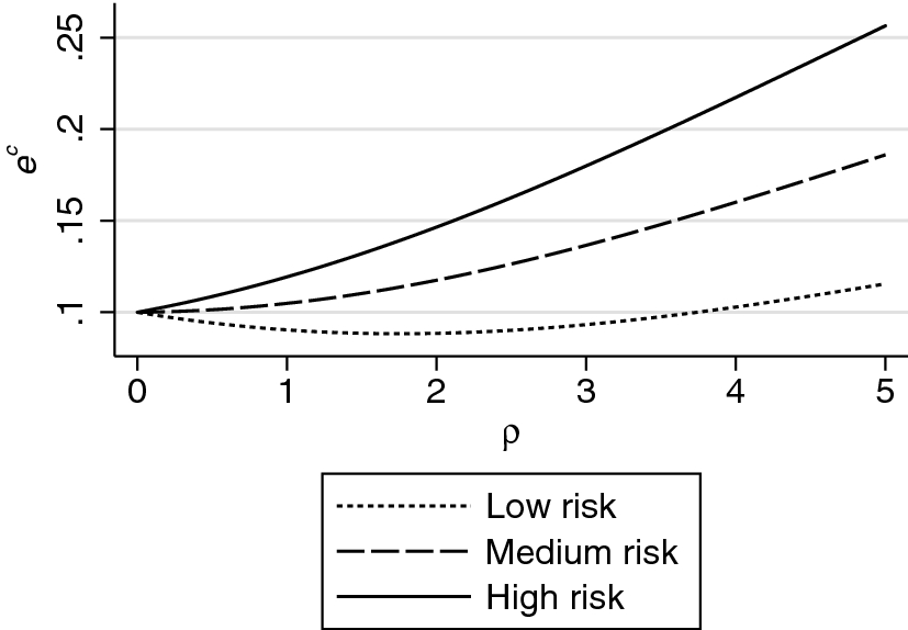
Fig. 1 Critical values for the absolute risk reduction, represented by e ^c, above which prevention is the optimal strategy for expected utility maximizing agents in the experiment. Figure shows critical value e ^c, the level of absolute risk reduction above which agents with a constant relative risk aversion utility function prefer prevention to non-prevention. All calculations are made under the assumption that agents maximize a CRRA utility function, that incomes in the high and low states are 20 and 10, respectively, and that the cost of prevention is 1. The risk levels in the low, medium and high risk environments are 0.3, 0.5, and 0.7, respectively

Two things are worth highlighting in the patterns displayed in Fig. 1. First, for a given absolute risk reduction (effectiveness), uptake of prevention decreases with the absolute level of risk. It is straightforward to see from inequality (2) that this must always be the case. For any concave utility function, the absolute utility cost of losing one unit of income in the bad state is strictly larger than the cost in the good state; higher absolute risk means that the relative likelihood of more costly utility state increases, which pushes agents towards not adopting the technology.

Second, a higher degree of risk aversion does not necessarily imply a higher likelihood of investing in prevention. In medium and high risk environments, at the same level of risk without prevention, more risk-averse agents demand more effective technology. However, there is a U-shaped relationship between risk-aversion level and critical value in terms of the prior about technology effectiveness in a low risk environment.

2.2 Prior updating

We assume that the probability of getting sick without prevention is known to agents. If agents decide to adopt prevention, they can directly test and experience its effectiveness, and subsequently update their beliefs about its effectiveness. Let ${\overline{e}}_{i,t}$ be the agent’s prior. If agents are Bayesian, they revise their beliefs about the effectiveness of the technology after a prevention outcome (either sick or healthy) $O\in \{PS,PH\}$ according to the formula:

(10) $\begin{array}{c}{f}_{i,t+1}\left(e_j\right)=P\left(e_j|O\right)=\frac{P\left(O|e_j\right)f_t\left(e_j\right)}{{\sum }_{k}P\left(O|e_k\right)f_t\left(e_k\right)}\end{array}$

In the case of a preventive failure, the revised belief will be:

(11) $\begin{array}{c}{f}_{i,t+1}\left(e_j\right)=P\left(e_j|PS\right)=\frac{\left(p-e_j\right)f_{i,t}\left(e_j\right)}{{\sum }_i\left(p-e\right)f_{i,t}\left(e_i\right)}=\frac{\left(p-e_j\right)f_{i,t}\left(e_j\right)}{p-{\overline{e}}_{i,t}}\end{array}$

(12) $\begin{array}{c}{\overline{e}}_{i,t+1}=\sum _j{e}_j{f}_{t+1}\left(e_j\right)=\frac{{\sum }_j{e}_j\left(p-e_j\right)f_{i,t+1}\left(e_j\right)}{p-{\overline{e}}_0}=\frac{p{\overline{e}}_{i,t}-E_{i,t}\left(e^2\right)}{p-{\overline{e}}_{i,t}}\end{array}$

where $E_{i,t}\left(e^2\right)$ is the expectation of e ² before new information arrives.

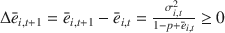
Negative experiences (preventive failure) will lead to weakly negative adjustment in beliefs:

(13) $\begin{array}{c}\Delta {\overline{e}}_{i,t+1}={\overline{e}}_{i,t+1}-{\overline{e}}_{i,t}=\frac{p{\overline{e}}_{i,t}-E_{i,t}\left(e^2\right)}{p-{\overline{e}}_{i,t}}-{\overline{e}}_{i,t}=\frac{-{\sigma }_{i,t}^2}{p-{\overline{e}}_{i,t}}\le 0\end{array}$

In the case of a prevention success, the revised belief will be:

(14) $\begin{array}{c}{f}_{i,t+1}\left(e_j\right)=P\left(e_j|PH\right)=\frac{\left(1-p+e_j\right)f_{i,t}\left(e_j\right)}{1-p+{\overline{e}}_{i,t}}\end{array}$

(15) $\begin{array}{c}{\overline{e}}_{i,t+1}=\frac{{\overline{e}}_{i,t}-p{\overline{e}}_{i,t}+E_{i,t}\left(e^2\right)}{1-p+{\overline{e}}_{i,t}}\end{array}$

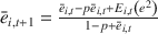
The adjustment in belief will be weakly positive:

(16) $\begin{array}{c}\Delta {\overline{e}}_{i,t+1}={\overline{e}}_{i,t+1}-{\overline{e}}_{i,t}=\frac{{\sigma }_{i,t}^2}{1-p+{\overline{e}}_{i,t}}\ge 0\end{array}$

In the experiment, subjects could test each technology over multiple time periods. Consider a sequence of R prevention outcomes $O=(O_1,O_2,\dots ,O_R)$ with S failures and H successes where S + H = R. The agent’s updated belief will be:

(17) $\begin{array}{c}{f}_{i,t+R}\left(e_j\right)=\frac{{\left(p-e_j\right)}^S{\left(1-p+e_j\right)}^H{f}_{i,t}\left(e_j\right)}{{\sum }_k{\left(p-e_k\right)}^S{\left(1-p+e_k\right)}^H{f}_{i,t}\left(e_k\right)}\end{array}$

(18) $\begin{array}{c}{\overline{e}}_{i,t+R}=\frac{{\sum }_j{\left(p-e_j\right)}^S{\left(1-p+e_j\right)}^H{e}_j{f}_{i,t}\left(e_j\right)}{{\sum }_k{\left(p-e_k\right)}^S{\left(1-p+e_k\right)}^H{f}_{i,t}\left(e_k\right)}\end{array}$

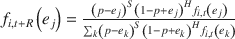
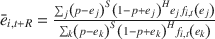
Proof

The agent iteratively revises his belief after each outcome:

(19) $\begin{array}{c}{f}_{i,t+1}\left(e_j\right)=P\left(e_j|O_1\right)=\frac{P\left(O_1|e_j\right)f_{i,t}\left(e_j\right)}{{\sum }_{k}P\left(O_1|e_k\right)f_{i,t}\left(e_k\right)}\end{array}$

(20) $f_{i,t+2}\left(e_j\right)=P\left(e_j|O_2\right)=\frac{P\left(O_2|e_j\right)f_{i,t+1}\left(e_j\right)}{{\sum }_{k}P\left(O_2|e_k\right)f_{i,t+1}\left(e_k\right)}=\frac{P\left(O_2|e_j\right)P\left(O_1|e_j\right)f_{i,t}\left(e_j\right)}{{\sum }_{k}P\left(O_2|e_k\right)P\left(O_1|e_k\right)f_{i,t}\left(e_k\right)}$

Similarly,

(21) $f_{i,t+R}\left(e_j\right)=P\left(e_j|O_R\right)=\frac{P\left(O_R|e_j\right)f_{i,t+R-1}\left(e_j\right)}{{\sum }_{k}P\left(O_R|e_k\right)f_{i,t+R-1}\left(e_k\right)}=\frac{{\prod }_{r}P\left(O_r|e_j\right)f_{i,t}\left(e_j\right)}{{\sum }_k{\prod }_{r}P\left(O_r|e_k\right)f_{i,t}\left(e_k\right)}$

Plugging $P\left(O_r|e_j\right)=p-e_j$ if $O_r=PS$ and $P\left(O_r|e_j\right)=1-p+e_j$ if $O_r=PH$ into Eq. (21), we have Eq. (17). Equation (18) follows.

Expression (18) is fairly intuitive: at any given time point (round), agents’ belief about the effectiveness of the technology depends on the risk level, their initial prior, and the number of prevention successes and failures they have experienced, independent of the temporal ordering of these outcomes.

3 Experimental design

In order to test our model predictions, we set up a lab experiment in which subjects were asked to decide whether to invest in a set of technologies lowering their risk exposure. In each round of the experiment, individuals had to decide whether to make an upfront investment into a preventive health technology, which would reduce the odds of falling sick, but not fully protect subjects against sickness. Subjects were asked whether they wanted to invest US$1 into prevention at the beginning of each period. If the player stayed healthy, the period income was 10 without prevention, and 9 with prevention; if the player fell sick, the period income was zero with prevention, and − 1 with prevention. While this full income loss may appear somewhat stark, health shocks are found to have an impoverishing impact in both developed and developing countries, even where the entire population is officially covered by a health insurance scheme (Wagstaff et al. Reference Wagstaff, Flores, Smitz, Hsu, Chepynoga and Eozenou2018; Wagstaff and van Doorslaer Reference Wagstaff and van Doorslaer2003). In the United States, sick days and basic medical expenses easily exceed monthly disposable incomes for uninsured populations (Dobkin et al. Reference Dobkin, Finkelstein, Kluender and Notowidigdo2018); even for populations with insurance, the utility loss associated with having to stay in bed for a week or having to undergo surgery may exceed the utility derived from a typical monthly income.

Each subject played 3 matches of 15 rounds each. Throughout the entire 45-round session, the risk environment was kept constant, while the effectiveness of the preventive technologies (called technologies A, B, and C) was separately randomized for each of the three matches. Complete instructions used in the lab are provided in Appendix B (Online Resource). Each player was informed about the probability of getting sick without prevention and that this risk level was constant throughout the entire session; we randomly exposed players to three risk settings: p = 0.3 (low risk), p = 0.5 (medium risk) and p = 0.7 (high risk).

Players were informed that the preventive technology “lower[ed] the probability of falling sick”, and that the three technologies were independent of each other and differed with respect to their effectiveness. Since the main idea of the experiment was to assess individual behavior in settings where prevention was effective but the exact effectiveness uncertain, the absolute risk reductions used in the lab were randomized between 0.12 and 0.20 across players and matches. Under both scenarios, prevention was designed to be welfare-improving: with the more moderate risk reduction of 0.12, the net expected benefit (or expected returns on investment) per round was 20 cents (a 12% increase of getting US$10 minus the US$1 upfront cost); with the larger risk reduction of 0.20, the net expected benefit of prevention was US$1 per round of play, which corresponds to an expected return on investment of 100%. We later refer to these as more and less effective prevention technologies.

Each subject was randomized into one of five message treatments, which was kept constant throughout the experiment, as outlined in Table 1 below. Individuals in the control treatment were informed that the technology decreased the probability of being sick but they were not informed that the technology had positive expected returns. Two treatments provided messages, but no information on actual probabilities, similar to the messages commonly used by public health professionals to encourage the adoption of new technologies, which tend not to give specific information about risk reduction. One of the treatments was strongly worded, the other acknowledged that preventive technology would fail when insurance was incomplete. In two other treatments, subjects received messages that revealed the effectiveness of the technology.

Table 1 Messages and information

	No messagea	Balanced message	Strong message
Diffuse prior on probabilitiesb	No additional text	“On average, prevention pays. There is still some risk to you that you will get sick even if you pay to prevent”	“On average, prevention pays. We strongly encourage you to buy this product”
Common prior on probabilitiesb	No additional text	With prevention, the probability of getting sick will be either <p − 0.2> or <p − 0.12>, with both being equally likely. There is still some risk to you that you will get sick even if you pay to prevent	With prevention, the probability of getting sick will be either <p − 0.2> or <p − 0.12>, with both being equally likely. We strongly encourage you to buy this product

^aAll subjects received the message “[]…you will be playing this game for 15 periods. In each period you will earn an income of US$ 10 if you stay healthy and an income of zero if you fall sick. The probability of falling sick in each period is constant at p = [x] (a [x] in 10 chance) over the game period. In each period you can invest in a preventive health technology for $1 which lowers the probability of falling sick”

^bIn the diffuse prior setting, subjects were only informed that the technology would lower the probability of falling sick; in the common prior, they were informed that the probability would either be p − 0.2 or p − 0.12 with equal probability (see full text above)

Both the risk environment and message treatment were kept the same for each subject throughout the full session (individual-level randomization). Because we wanted subjects to experience different technologies, technology effectiveness was randomized at the match level (i.e. 3 random effectiveness draws for each subject).

In the first two matches, subjects made decisions independently and could not observe others’ outcomes. In the third match, subjects were able to communicate with other players in their randomly assigned group. We limit our analysis to the first two matches in which subjects could not communicate their experiences. Analysis of the effects of communication on prevention decisions can be found in other work (Saran et al. Reference Saran, Fink and McConnell2018).

All subjects received a show-up fee of US$10. Subjects were informed that they would receive additional payments corresponding to the outcomes of one randomly selected round in each of three matches, where they would be sampling a different technology in each match. Across the three matches, subjects could thus earn an additional income between − 3 (prevented and got sick all three rounds) and + 30 (no prevention, never sick). Subjects were paid in cash at the end of the experiment. After completing all experimental games, subjects completed a comprehensive questionnaire shown in Appendix C (Online Resource). Besides demographic and socio-economic indicators, the questionnaire included questions about health behaviors in realistic health settings, a risk aversion module (Holt and Laury Reference Holt and Laury2002), a delay discounting module (Kirby et al. Reference Kirby, Petry and Bickel1999) and a financial literacy and sophistication questionnaire (Lusardi and Mitchell Reference Lusardi, Mitchell, Mitchell and Lusardi2011). We did not include ambiguity aversion measures though this would be useful to measure in future work.

The experiment was conducted at the Harvard Decision Sciences Laboratory with a total of 679 participants. All subjects were reminded that the laboratory does not allow any deception of subjects. As shown in Table 2, approximately 50% of all participants were assigned to the low risk environment (p = 0.3), which we considered the most likely scenario from a health perspective; the remaining 50% were split roughly equally across the medium (p = 0.5) and high risk (p = 0.7) settings; common priors treatments were only implemented for the high and low risk settings. Message and risk treatments were compared across subjects. Effective or non-effective technologies were randomly assigned in each “round” of play and therefore involve within subject comparisons. Table 3 shows a breakdown of participant characteristics by risk environments and by message treatments. The randomization process was fairly successful in balancing participant characteristics across treatments. However, statistically significant differences were observed for the p = 0.7 treatment which was introduced in the final stage of the experiment and was thus affected by differences in the subject pool over time. To address imbalance concerns, we control for subject characteristics in all regression models. We also show regression results without the p = 0.7 treatment condition in Appendix D of the online materials.

Table 2 Allocation of experimental treatments

Message treatment	Risk environmenT
	p = 0.3	p = 0.5	p = 0.7
No message	112	50	56
Balanced, diffuse priors	76		20
Strong, diffuse priors	90		28
Balanced, common priors	41	63	31
Strong, common priors	33	39	40
Total	352	152	175

Based on a total of 679 subjects. All risk and message treatments were held constant across the 45 rounds (15 rounds with each of the three technologies offered) played by each subject. Message and risk treatments are randomized across subjects. More and less effective technologies are randomized within subjects

Table 3 Summary statistics on experiment subjects

Variables	All	Risk environments			F statistic (ANOVA)	Message treatments					F statistic (ANOVA)
		p = 0.3	p = 0.5	p = 0.7		No message	Balanced, diffuse priors	Strong, diffuse priors	Balanced, common priors	Strong, common priors
Age in years	31.2	33.0	33.0	26.1	18.04***	30.2	33.7	32.7	29.9	31.2	1.79
	(13.6)	(14.0)	(13.4)	(11.4)		(14.0)	(13.4)	(13.8)	(12.2)	(13.8)
Female	0.48	0.50	0.47	0.47	0.35	0.47	0.45	0.53	0.50	0.48	0.49
White	0.54	0.57	0.53	0.48	1.84	0.54	0.53	0.60	0.49	0.54	0.81
African American	0.14	0.12	0.15	0.17	1.03	0.14	0.15	0.11	0.19	0.11	1.25
Asian American	0.14	0.13	0.11	0.17	1.28	0.12	0.17	0.15	0.11	0.15	0.63
Hispanic	0.06	0.04	0.08	0.07	1.77	0.08	0.04	0.03	0.07	0.05	0.87
College (some or completed)	0.63	0.62	0.55	0.71	4.74***	0.64	0.63	0.58	0.65	0.63	0.49
Graduate education	0.29	0.32	0.34	0.21	4.46**	0.26	0.32	0.37	0.26	0.29	1.47
Currently a student	0.53	0.47	0.46	0.70	15.19***	0.57	0.46	0.50	0.53	0.54	0.93
Currently married	0.11	0.11	0.14	0.09	1.13	0.09	0.15	0.14	0.13	0.08	0.79
Has children	0.14	0.14	0.18	0.09	3.44**	0.15	0.14	0.11	0.15	0.13	0.34
Height (cm)	171.4	171.2	171.7	171.5	0.12	171.6	172.3	169.7	172.0	171.0	1.01
	(11.1)	(11.1)	(10.8)	(11.5)		(11.2)	(11.1)	(10.1)	(10.9)	(12.2)
Weight (kg)	72.0	72.6	72.6	70.3	1.07	71.7	74.7	70.3	72.7	71.4	0.97
	(17.8)	(18.1)	(18.6)	(16.2)		(17.9)	(18.8)	(17.0)	(18.6)	(16.2)
Overweight $(\text{BMI}\ge 25)$	0.35	0.37	0.34	0.34	0.28	0.34	0.45	0.34	0.35	0.31	1.19
Obese $(\text{BMI}\ge 30)$	0.11	0.13	0.13	0.07	2.49*	0.10	0.13	0.14	0.13	0.10	0.37
Currently smoking	0.13	0.14	0.16	0.11	0.87	0.13	0.09	0.14	0.15	0.14	0.44
Currently taking vitamins	0.43	0.41	0.48	0.43	1.01	0.38	0.44	0.46	0.45	0.48	1.00
Flu shot in the last 12 months	0.47	0.44	0.49	0.51	1.23	0.51	0.43	0.47	0.44	0.44	0.89
Dentist visit in the last 12 months	0.78	0.78	0.76	0.79	0.15	0.78	0.77	0.81	0.79	0.71	0.91
Uses sunscreen regularly	0.39	0.40	0.45	0.31	3.26**	0.35	0.31	0.44	0.44	0.40	1.68
Attention score	1.34	1.31	1.15	1.55	5.11***	1.31	1.33	1.43	1.25	1.40	0.50
	(1.17)	(1.15)	(1.14)	(1.20)		(1.17)	(1.13)	(1.14)	(1.20)	(1.18)
Financial literacy score	3.95	3.91	4.05	3.94	0.60	3.89	3.84	3.90	4.11	4.01	0.82
	(1.38)	(1.45)	(1.25)	(1.33)		(1.44)	(1.52)	(1.26)	(1.35)	(1.28)
Risk aversion score	4.87	4.90	4.84	4.83	0.06	4.75	4.90	4.92	4.90	4.99	0.24
	(2.33)	(2.44)	(2.33)	(2.13)		(2.36)	(2.40)	(2.41)	(2.39)	(2.09)
Kirby discounting score	10.72	11.08	10.47	10.21	1.49	10.61	11.34	10.18	11.12	10.51	0.75
	(5.81)	(5.79)	(5.66)	(5.98)		(6.08)	(6.04)	(5.86)	(5.50)	(5.43)
Observations	679	352	152	175		218	96	118	135	112

The table displays means and standard deviations (in parentheses) unless indicated otherwise

***p < 0.01; **p < 0.05; *p < 0.1

In order to understand how experimental subjects learned about and evaluated the “quality” of the health technology, all subjects were asked to answer three simple questions regarding the technology at the end of each match of 15 rounds: whether respondents tried out the technology, if yes, how respondents would rate the technology effectiveness on a scale from 1 (“Bad”) to 4 (“Very good”), and whether respondents would recommend the technology observed to others.

4 Empirical specifications and results

Overall, a high proportion of subjects chose to prevent in the experiment. In the first two matches, the average prevention rate was 70%, differing slightly across risk environments. In the low-risk environment, the prevention rate was 70%. In the medium- and high-risk environments, the prevention rates were 67% and 74%, respectively. Subjects were more likely to adopt prevention when assigned more effective technologies. The corresponding prevention rates with more effective and less effective technologies were 72% and 68%. As shown in Fig. 2, the difference in prevention rates between those who received more effective and those who received less effective technologies emerged gradually within the first five rounds and remained clearly visible in the following rounds.

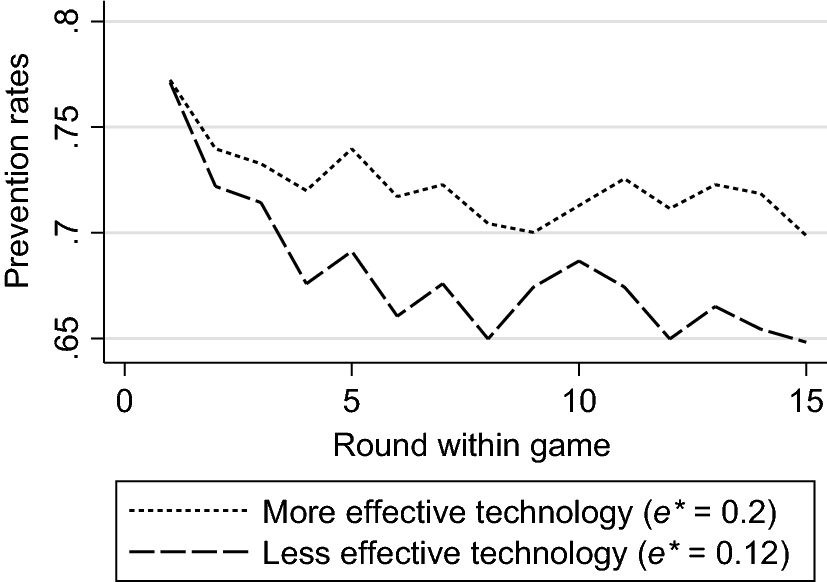
Fig. 2 Average prevention rates with more effective and less effective technologies

In Table 4 we show average preventive behavior during the laboratory experiment for subjects reporting and not-reporting each specific preventive behavior. For all of the behaviors except using sunscreen, we see that individuals who engaged in lab prevention had higher rates of self-reported prevention than individuals who did not prevent in the lab. These findings suggest that our experiment was capturing a tendency to engage in health prevention that is relevant across a variety of health domains.

Table 4 Self-reported preventive behavior and preventive behavior in the lab

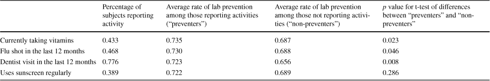
	Percentage of subjects reporting activity	Average rate of lab prevention among those reporting activities (“preventers”)	Average rate of lab prevention among those not reporting activities (“non-preventers”)	p value for t-test of differences between “preventers” and “non-preventers”
Currently taking vitamins	0.433	0.735	0.687	0.023
Flu shot in the last 12 months	0.468	0.730	0.688	0.046
Dentist visit in the last 12 months	0.776	0.723	0.656	0.008
Uses sunscreen regularly	0.389	0.722	0.689	0.286

All statistics are at the individual level, representing 679 study participants

Sending subjects health messages has a positive effect on prevention behaviors, raising the average technology adoption rate from 66.13 to 72.21%. Strong messages which do not reveal technology effectiveness seem to have the strongest effect—the average adoption rate in this treatment was 74.38%. The adoption rates in the other message treatments were 71.46%, 71.16%, and 71.85% for balanced messages without probabilities, balanced messages with probabilities, and strong messages with probabilities, respectively (Table 5).

Table 5 Prevention rates across treatments

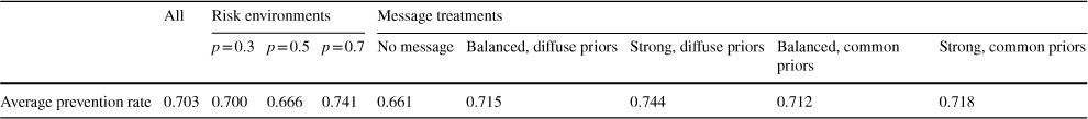
	All	Risk environments			Message treatments
		p = 0.3	p = 0.5	p = 0.7	No message	Balanced, diffuse priors	Strong, diffuse priors	Balanced, common priors	Strong, common priors
Average prevention rate	0.703	0.700	0.666	0.741	0.661	0.715	0.744	0.712	0.718

On average, in each match, about 53% of participants rated the technology as effective (either “quite effective” or “highly effective”). Subjects were eleven percentage point more likely to think the technology was effective if the absolute risk reduction was 0.2 rather than 0.12. They were also two percentage points more likely to rate the technology positively in the second match than they were in the first match.

We start our empirical investigation by analyzing our first theoretical prediction (Hypothesis H1), which states that population level prevention rates should weakly decline with rational updating of priors over time. Figure 3 shows that this is generally true. In the first match, initially about 79% of all subjects chose prevention; however, the prevention rate dropped to roughly 66% by round 15. In the second match, the decline in prevention rate was more gradual, from 75% in the first round to 69% in the fifteenth round.

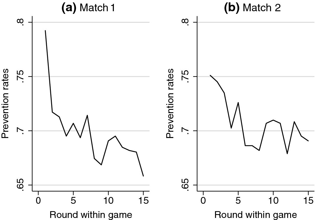
Fig. 3 Average prevention rates over time

We hypothesized that messages would increase prevention rates initially, but the effect would fade over time as subjects gained more personal experience (Hypothesis H2). We test this hypothesis by estimating

(22) $\begin{array}{cc}Prevent{s}_{i,r,g}& ={\beta }_0+{\beta }_{1}Messag{e}_i+{\beta }_{2}Messag{e}_i\ast Roun{d}_r+{\beta }_{3}Roun{d}_r+{\beta }_{4}MediumRis{k}_i\\ & +{\beta }_{5}HighRis{k}_i+{\beta }_{6}Effectiv{e}_{i,g}+{\gamma }^{\prime }{x}_i+{\delta }_g+{\epsilon }_{i,r,g}\\ \end{array}$

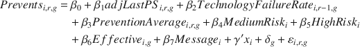
to estimate message impact differences across rounds, and by estimating

(23) $\begin{array}{cc}Prevent{s}_{i,r,g}& ={\beta }_0+{\beta }_{1}Messag{e}_i+{\beta }_{2}Messag{e}_i\ast Matc{h}_g+{\beta }_{3}MediumRis{k}_i\\ & +{\beta }_{4}HighRis{k}_i+{\beta }_{5}Effectiv{e}_{i,g}+{\gamma }^{\prime }{x}_i+{\delta }_g+{\epsilon }_{i,r,g}\\ \end{array}$

to analyze differences between matches. In both models, β ₁ captures the immediate message effect; β ₂ captures the changes in messaging effects over time. Prevents is a binary indicator for whether or subject i decided to invest into prevention in round r of match g; Message is an indicator variable indicating that any “public health” message was received, Round indicates round number; MediumRisk and HighRisk capture p = 0.5 and p = 0.7; Effective is a binary indicator for effective technology (probability reduction of 0.20 rather than 0.12), x _i is a vector of subject characteristics (age, sex, ethnicity, education, marital status, risk aversion score, discounting score,…) and δ _g is match (1–2) fixed effects (with match 1 as reference category).

Table 6 shows the results of this estimation. Columns 1–2 shows the effect of messages in the first five rounds and in the last ten rounds of both matches, columns 4–5 shows the effect of messages in the first and the second matches separately. Columns 3 and 6 directly test the models above, showing the interaction between message and round (column 3) and the interaction between message and match (column 6). Confirming our hypothesis, we find that messages have a positive impact on average, boosting prevention by about 6 percentage points. Columns 3 and 6 indicate that, although prevention rates tend to decrease round-by-round, the effect of messages does not fade within the match. Interestingly, we find much weaker and insignificant effects of public messaging in match 2, which could be interpreted as evidence for public health messages losing importance over time as subjects receive highly similar (or identical) messages with different technologies.

Table 6 Effects of messages

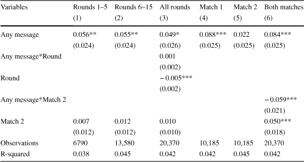
Variables	Rounds 1–5	Rounds 6–15	All rounds	Match 1	Match 2	Both matches
	(1)	(2)	(3)	(4)	(5)	(6)
Any message	0.056**	0.055**	0.049*	0.088***	0.022	0.084***
	(0.024)	(0.024)	(0.026)	(0.025)	(0.025)	(0.025)
Any message*Round			0.001
			(0.002)
Round			− 0.005***
			(0.002)
Any message*Match 2						− 0.059***
						(0.021)
Match 2	0.007	0.012	0.010			0.050***
	(0.012)	(0.012)	(0.010)			(0.018)
Observations	6790	13,580	20,370	10,185	10,185	20,370
R-squared	0.038	0.045	0.042	0.042	0.045	0.042

Robust standard errors in parentheses clustered at the individual level. All estimations control for subject characteristics (age group: 17–25, 18–40, 41–60, 61 and above, sex, ethnicity, education, whether the subject is a student, marital status, whether the subject is a parent, attention score, financial literacy score, risk aversion score, Kirby discounting score), and include fixed effects for risk levels and technology effectiveness (not reported)

***p < 0.01; **p < 0.05; *p < 0.1

We continue by testing Hypothesis H3, which states that in higher risk environments agents respond less to a preventive failure. We do this empirically by testing the following model:

(24) $\begin{array}{cc}Prevent{s}_{i,r,g}& ={\beta }_0+{\beta }_{1}TechnologyFailureRat{e}_{i,r,g}+{\beta }_{2}TechnologyFailureRat{e}_{i,r,g}\ast MediumRis{k}_i\\ & +{\beta }_{3}TechnologyFailureRat{e}_{i,r,g}\ast HighRis{k}_i+{\beta }_{4}PreventionAverag{e}_{i,r,g}\\ & +{\beta }_{5}MediumRis{k}_i+{\beta }_{6}HighRis{k}_i+{\beta }_{7}Effectiv{e}_{i,g}+{\beta }_{8}Messag{e}_i+{\gamma }^{\prime }{x}_i+{\delta }_g+{\epsilon }_{i,r,g}\\ \end{array}$

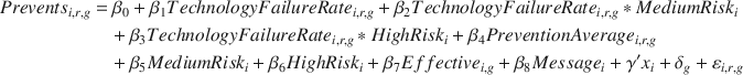
where TechnologyFailureRate is the rate of technology failures the subject has experienced in the previous rounds, PreventionAverage is the subject’s average rate of prevention in previous rounds, calculated by dividing the number of rounds with prevention by the number of rounds played. All other variables are defined as before.

Table 7 shows the main results from these regressions. Columns 1–3 show behavioral responses in low, medium and high risk environments separately. In all risk environments, agents reduce their prevention because of sickness experienced when prevention was chosen in previous rounds; however, this response is smaller in medium and high risk environments. In columns 4–6 we test the pooled model with interaction terms outlined in Eq. (24). Column 4 shows the results for the initial rounds 2–5, column 5 for the last rounds 6–15, and column 6 shows the results for all rounds 2–15. Despite the somewhat mixed pattern during the first few rounds, we find the anticipated positive interaction effects between observed prevention outcomes and medium risk and high risk levels in later rounds. A ten percentage point increase in technology failure rate in the previous rounds reduced the likelihood of preventing in the following round by about 3.71 percentage points in the low risk environment. The same effect is 2.67 and 2.40 percentage points in the medium and high risk environments, respectively, both effects are statistically significant. For all rounds, this interaction effect is smaller.

Table 7 Risk levels and prior updating

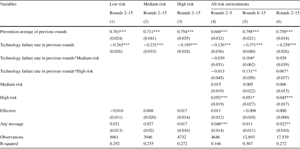
Variables	Low risk	Medium risk	High risk	All risk environments
	Rounds 2–15	Rounds 2–15	Rounds 2–15	Rounds 2–5	Rounds 6–15	Rounds 2–15
	(1)	(2)	(3)	(4)	(5)	(6)
Prevention average of previous rounds	0.763***	0.711***	0.754***	0.608***	0.798***	0.758***
	(0.024)	(0.041)	(0.035)	(0.032)	(0.021)	(0.018)
Technology failure rate in previous rounds	− 0.263***	− 0.231***	− 0.189***	− 0.126***	− 0.371***	− 0.258***
	(0.026)	(0.033)	(0.028)	(0.036)	(0.040)	(0.026)
Technology failure rate in previous rounds*Medium risk				− 0.039	0.104*	0.039
				(0.051)	(0.062)	(0.039)
Technology failure rate in previous rounds*High risk				− 0.013	0.131**	0.067*
				(0.045)	(0.058)	(0.037)
Medium risk				0.015	0.005	0.006
				(0.019)	(0.022)	(0.015)
High risk				0.052***	0.051*	0.045***
				(0.019)	(0.027)	(0.017)
Effective	− 0.010	0.008	0.017	0.011	− 0.008	0.000
	(0.011)	(0.020)	(0.014)	(0.012)	(0.010)	(0.008)
Any message	0.021	0.027	0.017	0.048***	0.011	0.022**
	(0.013)	(0.02)	(0.016)	(0.014)	(0.011)	(0.010)
Observations	8861	3946	4732	4646	12,893	17,539
R-squared	0.292	0.235	0.272	0.166	0.307	0.272

Robust standard errors in parentheses clustered at the individual level. All estimations control for subject characteristics (age group: 17–25, 26–40, 41–60, 61 and above, sex, ethnicity, education, whether the subject is a student, marital status, whether the subject is a parent, attention score, financial literacy score, risk aversion score, Kirby discounting score), and include fixed effects for matches 1–2 (not reported)

***p < 0.01; **p < 0.05; *p < 0.1

Hypothesis H4 looks more directly at updating of priors, and states that the behavioral response to adverse outcomes in any given round should be the same as the response to adverse outcomes in previous rounds. We test this hypothesis by using two alternative empirical models:

(25) $\begin{array}{cc}Prevent{s}_{i,r,g}& ={\beta }_0+{\beta }_{1}adjLastP{S}_{i,r,g}+{\beta }_{2}TechnologyFailureRat{e}_{i,r-1,g}\\ & +{\beta }_{3}PreventionAverag{e}_{i,r,g}+{\beta }_{4}MediumRis{k}_i+{\beta }_{5}HighRis{k}_i\\ & +{\beta }_{6}Effectiv{e}_{i,g}+{\beta }_{7}Messag{e}_i+{\gamma }^{\prime }{x}_i+{\delta }_g+{\epsilon }_{i,r,g}\\ \end{array}$

and

(26) $\begin{array}{cc}Prevent{s}_{i,r,g}& ={\beta }_0+{\beta }_{1}LastP{S}_{i,r,g}+{\beta }_{2}LastPS{2}_{i,r,g}+{\beta }_{3}PreventionAverag{e}_{i,r,g}+{\beta }_{4}MediumRis{k}_i\\ & +{\beta }_{5}HighRis{k}_i+{\beta }_{6}Effectiv{e}_{i,g}+{\beta }_{7}Messag{e}_i+{\gamma }^{\prime }{x}_i+{\delta }_g+{\epsilon }_{i,r,g}\\ \end{array}$

where LastPS and LastPS2 are indicators for whether technology failure happened last round and the round preceding it, respectively; TechnologyFailureRate _i,r-1,g is the technology failure rate in the previous rounds excluding the last round; adjLastPS is LastPS adjusted for (divided by) the number of previous rounds where technology was chosen (excluding the last round) to make β ₁ and β ₂ comparable.

The first model compares response to the most recent outcome with response to all other previous outcomes among those who prevented last round. The second model compares response to the most recent outcome with response to the outcome just preceding it among those who prevented in the two previous rounds.

Table 8, column 1, reports the effect of technology failure occurring in the last (preceding) round and the effect of all other previous technology failures in the match. Both variables are adjusted by the number of previous rounds with prevention. The probability of preventing drops by about 1.4 percentage points following a ten percentage point increase in technology failure rate in all previous rounds excluding the last round. The response to sickness experienced with prevention in the immediate past is also negative but substantially (and statistically) larger in magnitude ( $F=24.04,p<0.01$ ). Column 2 compares the effect of sickness in the previous round with sickness two rounds before among those who prevented in both rounds. The response to sickness in the preceding round is once again much larger than the response to sickness experienced two rounds before ( $F=7.12,p<0.01$ ).

Table 8 Weighting of outcomes

Variables	All individuals	Individuals preventing in the last 2 rounds
	(1)	(2)
Technology failure in the preceding round	− 0.323***
(adjusted for number of previous rounds where prevention chosen)	(0.034)
Technology failure rate in previous rounds	− 0.137***
	(0.023)
Technology failure in the preceding round		− 0.091***
		(0.009)
Technology failure 2 rounds before		− 0.059***
		(0.008)
Prevention average of previous rounds	0.641***	0.598***
	(0.029)	(0.038)
Medium risk	0.015	− 0.003
	(0.012)	(0.012)
High risk	0.057***	0.036***
	(0.012)	(0.010)
Effective	0.002	0.001
	(0.008)	(0.007)
Any message	0.014	0.013
	(0.009)	(0.009)
Observations	12,348	10,547
R-squared	0.186	0.130

Robust standard errors in parentheses clustered at the individual level. All estimations control for subject characteristics (age group: 17–25, 26–40, 41–60, 61 and above, sex, ethnicity, education, whether the subject is a student, marital status, whether the subject is a parent, attention score, financial literacy score, risk aversion score, Kirby discounting score), and include fixed effects for matches 1–2 (not reported)

***p < 0.01; **p < 0.05; *p < 0.1

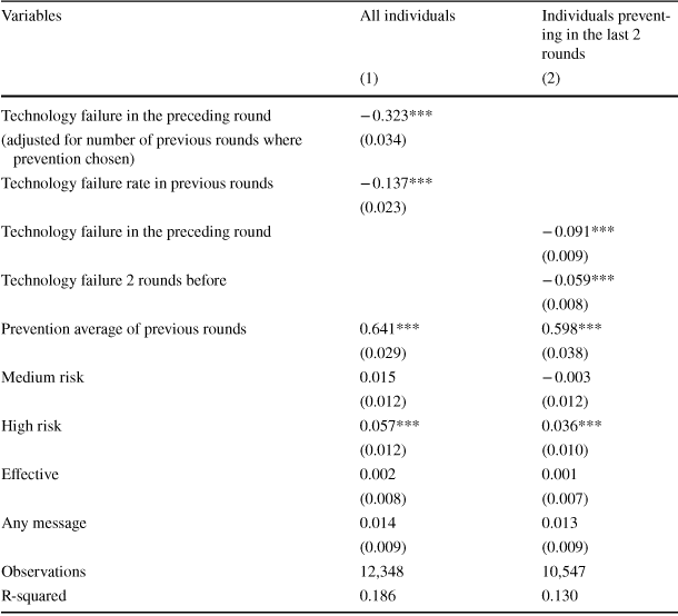
Finally, we test Hypothesis H5, which says that outcomes from non-prevention contain no information, and thus should not result in any updating. This hypothesis has three directly testable predictions. First, agents who opt against prevention in the first round should never choose prevention in subsequent rounds (H5a). Figure 4 shows the percentage of agents who did not prevent in the first round switched to prevention for the first time in later rounds. The percentage of subjects switching declines over time, but remains above zero in most rounds.

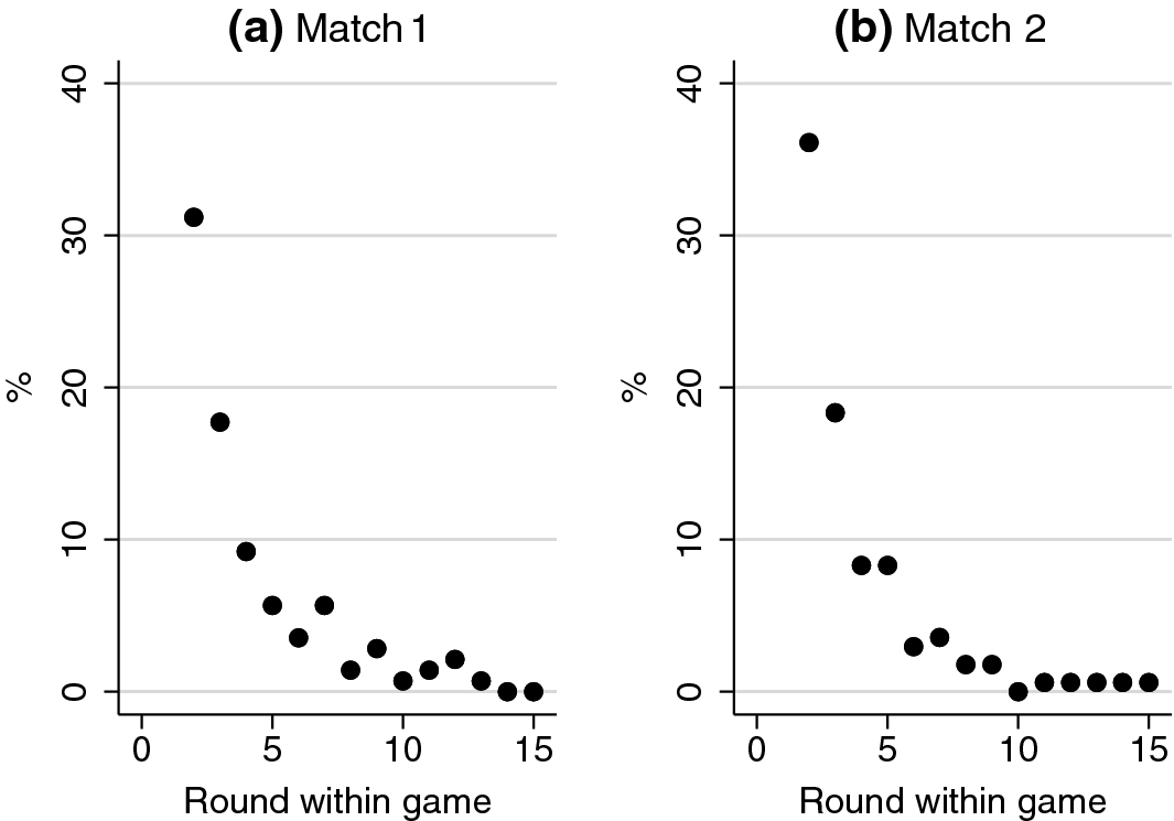
Fig. 4 Percentage of subjects not preventing in the first round switching to prevention for the first time in each round

Another important implication of rational prior updating is subjects who switch out of prevention due to negative experiences should never adopt prevention again because non-prevention contains no information about effectiveness (H5b). In Fig. 5, we show the percentage of subjects who prevented in the first round and did not prevent in the previous round switched to prevention the current round. Contrary to rational learning models we find that in every single round at least 30% of subjects who had abandoned the technology switched back to prevention.

Fig. 5 Percentage of subjects preventing in the first round and not preventing in the previous round switching to prevention in each round

Finally, we hypothesized that agents’ assessment of technology effectiveness would be independent of non-prevention outcomes (H5c). We investigate players’ assessment at the end of the trial period using the following empirical model:

(27) $\begin{array}{cc}Assessmen{t}_{i,g}& ={\beta }_0+{\beta }_{1}adjP{S}_{i,g}+{\beta }_{2}adjN{S}_{i,g}+{\beta }_{3}Preventio{n}_{\mathrm{ig}}+{\beta }_{4}MediumRis{k}_i\\ & +{\beta }_{5}HighRis{k}_i+{\beta }_{6}Effectiv{e}_{i,g}+{\beta }_{7}Messag{e}_i+{\gamma }^{\prime }{x}_i+{\delta }_g+{\epsilon }_{i,g}\\ \end{array}$

where Assessment is the subject’s overall rating of the effectiveness of the technology (1 = “Bad”, 4 = “Very good”), adjPS and adjNS are the number of failures experienced with and without prevention in the match, divided by the number of rounds with and without prevention, respectively. Prevention is the number of rounds where prevention was chosen.

Table 9 shows factors affecting subjects’ assessment of the technology. Columns 1–2 show the results for both matches, controlling and not controlling for risk levels. Columns 3–4 show the results for each match. In line with our hypothesis, subjects rate the technology as less effective if they experienced more technology failures in the match but on average their assessment is independent of non-prevention outcomes. Consistent with rational learning, subjects’ subjective technology assessment in general does not respond to health outcomes without prevention, despite their somewhat mild reaction in the first match. Given that we see large behavioral responses to non-prevention outcomes, this suggests that at least a part of the behavioral response is not directly linked to priors regarding technology effectiveness.

Table 9 Non-prevention outcomes and assessment

Variables	Both matches	Both matches	Match 1	Match 2
	(1)	(2)	(3)	(4)
Number of rounds where prevention chosen and sickness experienced	− 2.052***	− 2.036***	− 2.113***	− 2.018***
(adjusted for total number of rounds where prevention chosen)	(0.187)	(0.136)	(0.177)	(0.189)
Number of rounds where prevention not chosen and sickness experienced	0.043	0.044	0.325**	− 0.195
(adjusted for total number of rounds where prevention not chosen)	(0.129)	(0.123)	(0.162)	(0.170)
Number of rounds where prevention chosen	0.089***	0.090***	0.077***	0.100***
	(0.009)	(0.009)	(0.013)	(0.013)
Effective	− 0.030	− 0.029	− 0.077	0.005
	(0.062)	(0.062)	(0.087)	(0.089)
Any message	− 0.027	− 0.029	0.027	− 0.075
	(0.069)	(0.068)	(0.089)	(0.093)
Medium risk	− 0.057
	(0.097)
High risk	0.027
	(0.116)
Match 2	0.093*	0.093*
	(0.053)	(0.053)
Observations	836	836	422	414
Sample mean	3.228	3.228	3.184	3.273
R-squared	0.398	0.397	0.383	0.431

Robust standard errors in parentheses clustered at the individual level. All estimations control for subject characteristics (age group: 17–25, 26–40, 41–60, 61 and above, sex, ethnicity, education, whether the subject is a student, marital status, whether the subject is a parent, attention score, financial literacy score, risk aversion score, Kirby discounting score)

***p < 0.01; **p < 0.05; *p < 0.1

5 Discussion and conclusions

In this paper, we present a theoretical model of preventive technology adoption and test it through a series of incentivized lab experiments. The model yields several insights; first, choosing not to take up an effective (income-increasing) preventive technology is consistent with expected-utility maximization if priors are sufficiently diffuse and agents are risk-averse; second, prevention will likely decline over time as subjects who have negative experiences with prevention downgrade their priors and switch out of prevention; third, declines in prevention over time will be particularly large if baseline risk is small.

Overall, we find subjects’ behavior consistent with the predictions of our model. A substantial fraction of subjects did not prevent in the laboratory, even when they were informed that prevention is highly effective. We also observe a gradual decrease in prevention rates over time. After 15 rounds, the number of subjects choosing prevention dropped by 6–13 percentage points in each match. Individuals who have high expectations about the effectiveness of the technology initially adopt prevention, but later revise their expectations downward when the technology fails. We also observe that in higher risk environments subjects adjust their priors less in response to a technology failure in later rounds, which is consistent with higher frequency of failures and thus lower informational content of each failure in these environments.

However, we also see substantial deviations from any model based around rational updating. Agents react stronger to their most recent experiences than to experiences more distant in the past even though these experiences do not have different informational value, in particular when it comes to preventive failure. This is in line with recent findings that an individual’s decision to take a flu shot most heavily depends on recent outcomes (Jin and Koch Reference Jin and Koch2018). In contrast with our experimental setup, probabilities of adverse events are of course not known in more realistic settings, which means that individuals may also update their priors regarding risks without prevention over time. Stronger reactions to recent outcomes in our experiment are consistent with the well documented “recency effect”, which suggests that people generally are more influenced by more recent information (Miller and Campbell Reference Miller and Campbell1959; Murdock Reference Murdock1962). While discounting of more distant events is somewhat hard to justify in our experimental setup, it could well be efficient in other settings and is thus not necessarily inconsistent with rational choice theory.

We also find strong evidence of behavioral responses to outcomes that do not reveal any information to participants. Specifically, we find that subjects experiencing negative health outcomes without prevention—the likelihood of which was known and completely unrelated to the preventive technology’s effectiveness—are more likely to switch to prevention than subjects experiencing positive health outcomes. Since non-prevention does not provide any information about the effectiveness of preventive technology (or the actual risk, which was held constant and known to all subjects), this strategy adjustment is hard to reconcile with learning models, but rather seems to be the result of a behavioral response (“reacting”) to undesired outcomes.

These patterns of behavior in our experiment resemble findings from recent observational studies which document strong reaction to subjective experiences. Individuals are substantially more likely to purchase flood insurance in the year after a bad flood (Gallagher Reference Gallagher2014). Investors with recent losses on the stock market appear more likely to no longer invest in stocks or to reduce their stock exposure (de Bondt and Thaler Reference de Bondt and Thaler1990). It is possible that individuals use events to update their risk priors in these real-life contexts; this mechanism was intentionally ruled out in our experiment.

Interestingly, we find a discrepancy between subjects’ assessment of technology effectiveness and their prevention behavior. Assessments of technology effectiveness appear to be largely independent of outcomes experienced without prevention, the likelihood of which was known to subjects from the beginning of the experiment. This result is consistent with previous studies which often find that people assess likelihood in a Bayesian fashion (Anwar and Loughran Reference Anwar and Loughran2011; Liu and Hsieh Reference Liu and Hsieh1995). Yet in our experiments, subjects reacted more to non-prevention outcomes than rational models would predict, suggesting factors beyond the direct outcomes (such as the feelings those outcomes produce) may influence behaviors.

A possible explanation for why individuals react to illness, regardless of whether it is informative about the value of prevention is the “availability heuristic” (Tversky and Kahneman Reference Tversky and Kahneman1973), where recent experiences are most available (fresh in subjects’ mind) when subjects have to judge frequencies and probabilities, regardless of how much information these experiences contain. Our finding could also be explained by “experiential regret aversion” (Lovelady Reference Lovelady2014). While many models have focused on how regret and the anticipation of regret may shape decisions (Bell Reference Bell1982; Hayashi Reference Hayashi2011; Loomes and Sugden Reference Loomes and Sugden1987; Sarver Reference Sarver2008), “experiential regret aversion” focuses on how past feelings of regret influence future choices (Lovelady Reference Lovelady2014). In our experiment, regret could explain why individuals who fell sick in the experiment after failing to prevent switched strategies and became more likely to prevent. It is also possible that subjects play rationally only with some probability and experiment otherwise—developing new models to accommodate such behavior could be an interesting avenue for future work.

From a public policy perspective, our findings have three main implications: first, initial uptake of preventive technologies may be easier if the risk of adverse health outcomes is sufficiently large, or is at least perceived to be sufficiently large. Our results suggest that highlighting the risk of not engaging in prevention will likely increase uptake of prevention, at least in early stages when subjects have not yet gained experience with the technology.

The second main implication of our study is that the degree to which rates of prevention can be sustained over time is likely to be strongly affected by how likely adverse events are with prevention, or how imperfectly prevention protects against poor outcomes. While our experiment cannot fully capture long-term dynamics, it strongly suggests that negative experiences with preventive technologies have lasting effects on uptake. In some fortunate cases preventive technologies may be so effective that the likelihood of adverse health outcomes is very small; in those cases, uptake and adoption should be more easily sustained. In many other settings, including flu shots, bed nets or hygiene intervention, the same is clearly not true, so that a large number of individuals trying out the technology may choose to no longer pursue prevention after a certain number of failed trials.

The third and likely most positive finding is that public health messages can increase uptake of preventive technologies, even though the magnitude of these effects is not large—an increase of about 10% relative to the group without messages in our setting. Both the direction and magnitude of our finding are consistent with existing evidence on messaging in public health (Orr and King Reference Orr and King2015).

Our study has a few important limitations. First, we consider our results through a lens of expected utility maximization. Future work could consider alternative models such as minimax (Manski Reference Manski2020), which allow for the possibility that choices within the health sphere may reflect a different set of optimization criteria. Relatedly, the structure of our experimental setup is such that losses in the game are only possible when subjects choose to prevent. If subjects are averse to losses, our results may in part reflect a high prioritization of avoiding losses. In part, this design choice reflected the challenge of simulating losses in laboratory experiments (Hvide et al. Reference Hvide, Lee and Odean2019), which also limits our ability to study different illness severity within our setup. This is an area that could be very interesting for future studies. Third, for simplicity, we rule out spillover or contagion effects in the model, i.e. assume the risk of getting sick is independent of other people’s preventive efforts. In practice, this is clearly not the case in many real world settings, where disease risk directly increases with the risk of other people not preventing (e.g. measles, flu but also general hygiene behaviors). In these settings, our model could be viewed as a special case where individuals take the behavior of other people in their surrounding as given; similar results would likely also emerge if dynamic interactions would be considered, although such a model would be much harder to solve.

Overall, our results suggest that, in settings where individuals’ repeated investments are necessary for positive health outcomes, it may be worthwhile to spend greater resources developing preventive strategies that are highly effective instead of spending resources on promoting preventive technologies that are only partially effective. For technologies with relatively high probabilities of preventive failure, stronger external measures such as financial incentives, social pressure or legal requirement may be necessary to achieve high rates of adoption over time.