Images say more than just words: visual versus text communication to dispel a rent-control misconception

Jordi Brandts; Isabel Busom; Cristina Lopez-Mayan; Judith Panadés

doi:10.1007/s10683-023-09817-7

Images say more than just words: visual versus text communication to dispel a rent-control misconception

Published online by Cambridge University Press: 14 March 2025

and

Jordi Brandts*: Affiliation:
Instituto de Análisis Económico (CSIC) and Barcelona School of Economics, Barcelona, Spain
Isabel Busom: Affiliation:
Universitat Autònoma de Barcelona, Barcelona, Spain
Cristina Lopez-Mayan: Affiliation:
Serra Húnter Fellow and AQR-IREA, Universitat de Barcelona, Barcelona, Spain
Judith Panadés: Affiliation:
Universitat Autònoma de Barcelona and Barcelona School of Economics, Barcelona, Spain
*: jordi.brandts@iae.csic.es

Article contents

Abstract
Introduction
Experimental framework
Analysis
Results
Conclusions
Funding
Footnotes
References

Rights & Permissions

Abstract

The highly popular belief that rent-control leads to an increase in the amount of affordable housing is in contradiction with ample empirical evidence and congruent theoretical explanations. It can therefore be qualified as a misconception. We present the results of a preregistered on-line experiment in which we study how to dispel this misconception using a refutational approach in two different formats, a video and a text. We find that the refutational video has a significantly higher positive impact on revising the misconception than a refutational text. This effect is driven by individuals who initially agreed with it and depart from it after the treatment. The refutational text, in turn, does not have a significant impact relative to a non-refutational text. Higher cognitive reflective ability is positively associated with revising beliefs in all interventions. Our research shows that visual communication effectively reduces the gap between scientific economic knowledge and the views of citizens.

Keywords

Misconceptions Policy beliefs Communication Refutation Online experiments

JEL classification

A1: General Economics A2: Economic Education and Teaching of Economics D9: Micro-Based Behavioral Economics‡ C9: Design of Experiments D83: Search • Learning • Information and Knowledge • Communication • Belief • Unawareness

Type: Original Paper
Information: Experimental Economics , Volume 27 , Issue 2 , April 2024 , pp. 417 - 468

DOI: https://doi.org/10.1007/s10683-023-09817-7 [Opens in a new window]
Creative Commons: This is an Open Access article, distributed under the terms of the Creative Commons Attribution (CC-BY) license (http://creativecommons.org/licenses/by/4.0/), which permits unrestricted re-use, distribution, and reproduction in any medium, provided the original work is properly cited.
Copyright: Copyright © The Author(s) 2024

They [economists] are accused of all thinking the same thing. But what use would economists be if they could not reach a consensus about anything?

Jean Tirole, “Economics for the public good”, p. 65, Princeton University Press, 2017.

1 Introduction

Research on how to communicate economic research findings to the general public effectively is still limited. However, policymakers and researchers increasingly acknowledge the need to improve the communication of economic research results about how economic policies work (Stankova, Reference Stankova2019). Recently, some studies have started to approach this issue. For instance, Haldane and McMahon (Reference Haldane and McMahon2018) and Coibion et al. (Reference Coibion, Gorodnichenko and Weber2019, Reference Coibion, Gorodnichenko and Weber2020) analyze how communication of fiscal and monetary policies affects agents’ expectations, where communication becomes a policy tool in itself. Other studies focus on the spread of socio-economic misinformation in the media (“alt-facts”) and on the effect of fact-checking to neutralize it (Barrera et al., Reference Barrera, Guriev, Henry and Zhuravskaya2020; Ecker et al., Reference Ecker, O’Reilly, Reid and Chang2020; Henry et al., Reference Henry, Zhuravskaya and Guriev2021). Finally, some other studies analyze how people perceive and form their attitudes towards tax policy (Stantcheva, Reference Stantcheva2021), towards racial gaps (Alesina et al., Reference Alesina, Ferroni and Stantcheva2021) and towards unregulated price increases (Elias et al., Reference Elias, Lacetera and Macis2022).

Little is known, however, on how to communicate economic knowledge when large segments of the public have entrenched misconceptions—that is, beliefs that contradict well-established scientific knowledge about the functioning of the economy. The problem is that widespread unfounded beliefs, some of them derived from not accounting for equilibrium effects, may result in the public endorsing damaging economic policies, or rejecting the implementation of evidence-based, welfare-enhancing reforms (Nyhan, Reference Nyhan2020; Bó et al., Reference Bó, Bó and Eyster2018). Hence, it is of general interest to explore how to communicate convincingly economic research findings that contradict prevalent misconceptions.

We focus here on the popular belief that rent control allows more families to find affordable housing. The support for this policy is substantial among the public, above 60% in polls conducted in several countries.Footnote ¹ This belief, however, is at odds with scientific consensus arising from economic research. To illustrate, about 95% of economists in the IGM Economic Experts Panel strongly disagree that rent capping will increase the quantity of affordable housing.Footnote ²

This high consensus stems from the abundant and cumulative empirical evidence on this subject (see, for instance, Diamond et al. (Reference Diamond, McQuade and Qian2019a) and Kholodilin and Kohl (Reference Kholodilin and Kohl1839). Although rent control may have positive effects for a subset of tenants because their rents will be lower, or grow less, relative to market rents (Sims, Reference Sims2007), both total quantity of rental housing available and quality of controlled housing ends up falling (Sims, Reference Sims2007; Mora-Sanguinetti, Reference Mora-Sanguinetti2011; Asquith, Reference Asquith2019; Diamond et al., Reference Diamond, McQuade and Qian2019a; Hahn et al., Reference Hahn, Kholodilin and Waltl2021; Monràs & García-Montalvo, Reference Monràs and García-Montalvo2021; Ahern & Giacoletti, Reference Ahern and Giacoletti2022). Some owners decide not to rent their property but sell it instead, either to owner-occupants or to developers (Diamond et al., Reference Diamond, McQuade and Qian2019a). Supply reduction is more pronounced among corporate landlords than among individual landlords (Diamond et al., Reference Diamond, McQuade and Qian2019b). As the number of tenants willing to pay the controlled rent is higher than the supply of dwellings, queues and a black market for rental contracts appear (Malpezzi, Reference Malpezzi1998; Andersson & Söderberg, Reference Andersson and Söderberg2012).Footnote ³ In the end, low-income tenants—young people and newcomers—are most likely to be harmed by this policy (Hahn et al., Reference Hahn, Kholodilin and Waltl2021; Kattenberg & Hassink, Reference Kattenberg and Hassink2017). Alternative policies, however, such as increasing supply, or tax subsidies for low-income households, are welfare increasing (Diamond et al., Reference Diamond, McQuade and Qian2019b).

Research in communication and in social, educational and political psychology shows that a refutational correction can reduce the prevalence of misconceptions in a variety of domains, such as climate change (Nussbaum et al., Reference Nussbaum, Cordova and Rehmat2017; Lewandowsky, Reference Lewandowsky2021), education (Aguilar et al., Reference Aguilar, Polikoff and Sinatra2019), psychology (Kowalski & Taylor, Reference Kowalski and Taylor2009, Reference Kowalski and Taylor2017) and vaccine resistance (Lewandowsky et al., Reference Lewandowsky, Ecker, Seifert, Schwarz and Cook2012). The surge of misinformation associated with the recent Covid-19 pandemic and its consequences has prompted further research on debunking, showing that refutational corrections are effective at it (MacFarlane et al., Reference MacFarlane, Tay, Hurlstone and Ecker2021). The main features that characterize a refutational correction are that the misconception addressed is explicitly stated and declared as incorrect; the existing scientific arguments and evidence are explained as simply as possible, and the relevance of the issue for the individual and her values is explicitly acknowledged (Tippett, Reference Tippett2010; Druckman, Reference Druckman2015; Weil et al., Reference Weil, Schul and Mayo2020). In contrast, a non-refutational approach does not include all these elements, as it simply lays out in a neutral way the arguments that explain a fact or a relation. The refutational correction is an appealing approach because it aims at inducing careful, reflective thinking about the evidence and arguments provided by scientific research about the several dimensions of a problem. It is a thoughtful way to communicate counter-intuitive information that takes into account the affective elements behind some beliefs. This approach, however, has barely been studied in relation to popular misconceptions about economic policies.

In this paper we report a new study where we use this communication method to design an information treatment experiment aimed at reducing the prevalence of the misconception about the effects of rent control. We conduct a set of on-line survey experiments with three interventions, one visual and two text-only, and test the effectiveness of each format in dispelling the misconception.Footnote ⁴ Given that ultimately we are interested in engaging with ordinary citizens, whose beliefs affect their support for policies, we here use a new subject pool extracted from the general population that includes participants of all ages and conditions living in Spain. We recruit a sample of 1,050 participants who are randomly allocated to one of the three interventions and participate through their own digital devices.

We design two short text-only messages about the effects of rent controls. One of the messages—the refutational text (RT hereafter)—uses the refutational approach which includes the refutational features described above. The other message—the non-refutational text (NRT hereafter)—uses a standard expository approach. This text explains, in a neutral way, the effects of a rent control policy, much like how a standard textbook of introductory economics would do. The most distinctive feature of the NRT is that it does not include the refutational elements. These texts build on previous work by Brandts et al. (Reference Brandts, Busom, Lopez-Mayan and Panadés2022), where we test the effectiveness of two written messages in dispelling the rent control misconception. Two important differences are that in the previous study both texts were twice as long as the ones used here, and that participants were college students. In reducing the number of words of both texts, we aim at achieving a balance between providing an accurate explanation and minimizing the time and cognitive effort required to read them. This may increase the effectiveness of the text-only messages, in particular of the RT. Readers may not pay sufficient attention when a text is long; length may also be in the way of the refutational elements of the RT to be salient enough. Indeed, previous research in psychology finds that short textual information is effective to reduce the prevalence of factual misconceptions (Ecker et al., Reference Ecker, O’Reilly, Reid and Chang2020).

To design the visual message we build on research that suggests that using visual explanations, such as videos and infographics may be more effective than text-only information to correct misconceptions or misinformation (Mason et al., Reference Mason, Baldi, Ronco, Scrimin, Danielson and Sinatra2017; Mayer & Moreno, Reference Mayer and Moreno2003; Goldberg et al., Reference Goldberg, van der Linden, Ballew, Rosenthal, Gustafson and Leiserowitz2019; Young et al., Reference Young, Jamieson, Poulsen and Goldring2018; Reynolds et al., Reference Reynolds, Pilling and Marteau2018). Adding visual elements reduces the participants’ cognitive and attention effort required to process the new and counter-intuitive information. More broadly, visual presentations match more closely how citizens nowadays encounter information of different kinds. Our visual message includes the elements from the refutational approach. We produce a refutational video (RV, hereafter), which is a dynamic slideshow where frames combine text and images using the refutational framework. Specifically, the RV adds images and symbols to selected textual sentences from the RT, including all refutational elements.

We elicit participants’ beliefs before and after the corresponding treatment by asking them, on a 5-point Likert scale, about their degree of agreement with a statement that says that the establishment of rent controls increases the number of people who have access to housing. We transform the degrees of agreement into a numerical scale, and define our outcome variable as the difference between post-treatment and pre-treatment beliefs. With the term belief, we refer to the degree of agreement with the statement. The outcome of interest is, thus, the change in beliefs of each participant. We compare the effectiveness of the RV relative to the new short RT and NRT messages in reducing the prevalence of the rent-control misconception. We also compare the effectiveness of these two text messages to each other. We further explore whether the effect of information treatments on updating beliefs varies for different subgroups of participants according to relevant socio-demographic characteristics such as housing status (tenants vs owners), gender and education.

Aside from the informational treatment, a personality trait that may affect the change in beliefs, according to previous evidence, is an individual’s predisposition to reflective or to intuitive thinking as measured by the cognitive reflection test (CRT) (Pennycook & Rand, Reference Pennycook and Rand2019; Pennycook et al., Reference Pennycook, McPhetres, Zhang, Lu and Rand2020; Tappin et al., Reference Tappin, Pennycook and Rand2020). We thus analyze the role of this trait on the disposition to update beliefs, and whether it varies with the treatment.Footnote ⁵

Our work contributes to the still sparse literature on communicating counter-intuitive expert consensus about the effects of an economic policy to the general public. As explained above, an emerging literature addresses issues such as how to communicate inflation expectations by central banks, or how attitudes and preferences towards redistribution, taxation or immigration are determined. Very little is known, however, about how to credibly communicate the evidence about policy effects and whether communication formats make a difference. The use of the refutation approach to correct economic misconceptions, either using visual or text-only formats, has been underexplored, despite their application in psychology for correcting misperceptions, misconceptions and misinformation.

Our contribution is threefold. We provide first evidence in economics on the effectiveness of using a visual communication format combined with a refutational approach to dispel a widespread and highly persistent misconception. Although some authors have used visual formats—instructional videos—to increase financial education (Lusardi et al., Reference Lusardi, Samek, Kapteyn, Glinert, Hung and Heinberg2017) and awareness of the consequences of taxation for income distribution (Stantcheva, Reference Stantcheva2021), they have neither investigated their effectiveness in relation to causal misconceptions about policy effects, nor adopted a refutational approach. Concerning the beliefs about the rent-control policy, previous works study the effectiveness of informational treatments that rely on text-only messages (Brandts et al., Reference Brandts, Busom, Lopez-Mayan and Panadés2022; Dolls et al., Reference Dolls, Schüle and Windsteiger2022; Müller & Gsottbauer, Reference Müller and Gsottbauer2022).

Second, we provide evidence on the effectiveness of short texts, a step forward with respect to the evidence reported in Brandts et al. (Reference Brandts, Busom, Lopez-Mayan and Panadés2022), where texts are twice as long. In our new study described here, both short RT and NRT lead to a higher reduction in the prevalence of the misconception. Furthermore, this improvement is obtained with a sample of ordinary citizens—not college students—, who are the natural target for communicating economic policies. Third, we show evidence on whether the role of personality traits on revising the misconception varies across visual and written formats. Our study, thus, adds to an emerging research in economics on the effectiveness of different modes of communicating research findings that confront popular beliefs, as well as to the growing literature on debunking misconceptions in political and economic psychology, and, more broadly, to the literature on science communication.

Our main findings are as follows. First, the RV has a significantly higher impact on dispelling the misconception than the RT for participants who initially hold the misconception, that is, the main target group. The effect of the video is even higher relative to the non-refutational, expository text. Second, we do not find that the RT is more effective than the NRT, as both lead to a similar decline in the prevalence of the misconception. Third, a higher propensity to reflective thinking induces a change away from the misconception, for participants who initially hold it, in all treatments.

The paper is organized as follows. Section 2 explains the hypotheses, conditions and procedure of our experimental framework. Section 3 describes the specifications used to test the hypotheses. Section 4 reports the estimated treatment effects and the results of a heterogeneity analysis across some socio-demographic characteristics. Section 5 concludes.

2 Experimental framework

2.1 Research hypotheses

We test three hypotheses, as preregistered. Hypotheses one and two are our central hypotheses, since they pertain to the treatment effects of the RV, RT and NRT, while the third hypothesis refers to the role of cognitive traits. The first hypothesis is about the effect of using the video format on the change in beliefs:

Hypothesis 1 (H1): Communicating scientific evidence about rent control policy through a refutational video is more effective to dispel the misconception about this policy than a refutational or a non-refutational text.

H1 relies on literature from social and political psychology and from communication that has investigated the effects of different communication formats on recipients’ beliefs or attitudes regarding climate change, political or health issues. Some examples of this work, most of it experimental, are the following. Goldberg et al. (Reference Goldberg, van der Linden, Ballew, Rosenthal, Gustafson and Leiserowitz2019) report that a video is significantly more effective than its transcript in increasing people’s perception of scientific agreement on climate change. Bolsen et al. (Reference Bolsen, Palm and Kingsland2019) show that climate science politicization undermines credible textual frames, but that adding compelling imagery to the textual frames counteracts science politicization and restores the impact of a scientific consensus message. In a similar vein, Young et al. (Reference Young, Jamieson, Poulsen and Goldring2018) show that providing audiovisual information is more effective than text-based messages in correcting misperceptions in the context of political fact-checking. Reynolds et al. (Reference Reynolds, Pilling and Marteau2018) find that using infographics enhanced with images to communicate evidence on the effectiveness of a hypothetical tax to tackle childhood obesity increases perceived effectiveness and support for this policy. In the educational literature, Mayer and Moreno (Reference Mayer and Moreno2003) document that meaningful learning involves cognitive processing that includes building connections between pictorial and verbal representations. Mason et al. (Reference Mason, Baldi, Ronco, Scrimin, Danielson and Sinatra2017) find that accompanying a refutational text with a graph is more effective to reduce a misconception about the earth’s seasonal changes than the text alone. All this work suggests that explanations that include visual components may also be more effective than text-only messages in communicating the effects of economic policies, such as rent-control. Note that the cleaner part of H1 is to compare the RV with the RT, since both have the refutational elements, and only the format changes. For completeness, H1 includes the comparison with the NRT.Footnote ⁶

Our second hypothesis refers to the effect of a written refutational correction relative to a non-refutational written message:

Hypothesis 2 (H2): Communicating scientific evidence about rent control policy through a refutational text is more effective to dispel the misconception about this policy than a non-refutational text.

Evidence from psychological, political and educational research shows that a refutational correction is often more effective than a simple retraction to correct misinformation in domains such as climate change, educational policies and psychology (Kowalski & Taylor, Reference Kowalski and Taylor2009; Tippett, Reference Tippett2010; Lewandowsky et al., Reference Lewandowsky, Ecker, Seifert, Schwarz and Cook2012; Lewandowsky, Reference Lewandowsky2021; Chan et al., Reference Chan, Jones, Jamieson and Albarracín2017; Aguilar et al., Reference Aguilar, Polikoff and Sinatra2019; Ecker et al., Reference Ecker, O’Reilly, Reid and Chang2020; Weil et al., Reference Weil, Schul and Mayo2020). In economics, and in the case of the particular misconception about the effects of rent controls, Brandts et al. (Reference Brandts, Busom, Lopez-Mayan and Panadés2022) report mixed findings in this respect. In the laboratory experiment with college students, both their RT and NRT reduce the misconception on rent controls by a similar magnitude. Hence, the RT does not significantly improve on the NRT. However, in the field environment of a college course, the RT is more effective than standard, non-refutational instruction, and it also slightly improves on the NRT. Here we now test the effectiveness of the written refutational approach using shorter texts based on Brandts et al. (Reference Brandts, Busom, Lopez-Mayan and Panadés2022). Given the length of the texts in our previous paper, participants may not have been able to pay attention to the refutational elements of the RT. In a shorter RT the refutational elements may be more salient. Some previous studies show that short messages are effective. For instance, Ecker et al. (Reference Ecker, O’Reilly, Reid and Chang2020) find that refutational fact-checks (like Tweets) reduce misinformation regarding factual claims. Ferrero et al. (Reference Ferrero, Konstantinidis and Vadillo2020) show that 200-word—long texts reduce the number of misconceptions about education among teacher education students. Hypothesis 2 is aimed at assessing the sensitivity of our previous results to the shorter, less attention-demanding version of both texts.

Our third hypothesis refers to the association between the propensity to cognitive reflection and changes in beliefs:

Hypothesis 3 (H3): Higher cognitive reflection values—higher propensity to analytical thinking—will induce a higher positive change in the misconception.

We study the role of a particular personality trait, the inclination to reflective relative to intuitive thinking, on the change of beliefs after being exposed to each treatment. Understanding scientific reasoning and evidence requires cognitive effort, especially when people have misconceptions on an issue. The individual inclination to analytical thinking may thus affect the extent to which people revise their beliefs, as previous evidence shows. Measuring this trait through modified versions of the Cognitive Reflection Test, Pennycook and Rand (Reference Pennycook and Rand2019), Pennycook et al. (Reference Pennycook, McPhetres, Zhang, Lu and Rand2020) and Tappin et al. (Reference Tappin, Pennycook and Rand2020) find that an individual’s ability to discern fake news from real news, and to update beliefs about political issues, are positively correlated with higher propensity to use analytical thinking (higher CRT scores). Furthermore, McPhetres et al. (Reference McPhetres, Bago and Pennycook2020) find that cognitive sophistication is often positively correlated with pro-science beliefs, although political affiliation may affect this correlation for some divisive issues. Brandts et al. (Reference Brandts, Busom, Lopez-Mayan and Panadés2022) also report that higher CRT scores are positively related to revising the rent-control misconception in some, but not all, conditions. Given the length of the texts used in our previous paper, cognitive reflection perhaps could not make more of a difference there. Given this evidence, here we will account for this trait.

2.2 Conditions

The experiment has three conditions: the RV condition, the RT condition and the NRT condition. A first pre-analysis plan (PAP) was preregistered at AsPredicted Registry, Wharton Credibility Lab (University of Pennsylvania) on July 4, 2020. This PAP included the RT and NRT conditions. The PAP corresponding to the RV condition was preregistered at AsPredicted Registry on July 3, 2021. All three conditions were preregistered before running the corresponding experiments. Budgetary constraints prevented us from conducting the three conditions simultaneously. To avoid potential seasonal effects we conducted both experiments on the same day and month. Pandemic, socio-economic and political conditions were very similar over this period.Footnote ⁷

Conditions only differ in the format the message is delivered to participants. In the RV condition, participants watch a 2:42 minute long refutational video about the effects of the rent control policy. In the RT and NRT conditions, participants read a text about the same issue that uses, respectively, a refutational and a non-refutational approach. The estimated reading time of the NRT and the RT is about 2 and 3 minutes, respectively (see Table 11 in Appendix 2). Thus, all formats are designed to take the reader/viewer a similar amount of time.

We follow the guidelines from research in psychology in incorporating the refutational elements into the design of the RV and the RT (Tippett, Reference Tippett2010; Druckman, Reference Druckman2015; Lewandowsky, Reference Lewandowsky2021). The features that characterize the refutational approach are the following. First, the text must activate the misconception. Second, it must explicitly state that the misconception is incorrect. Third, it must explain, as simply and clearly as possible, the scientific arguments and evidence on the topic at hand to show why the misconception is incorrect and what the negative consequences of the belief are. Fourth, it must aim at capturing the recipient’s attention making clear the personal relevance of the problem and the connection with the person’s values.Footnote ⁸ As in Brandts et al. (Reference Brandts, Busom, Lopez-Mayan and Panadés2022) we add another feature, which is that we explain that alternative and effective policies to reach the same goal exist. Our intention is to show participants that there are effective policies aligned with fairness concerns, but without the negative consequences of a rent control policy.

2.2.1 The RT

The refutational text is, in Spanish, 671 words long. Based on the longer RT in Brandts et al. (Reference Brandts, Busom, Lopez-Mayan and Panadés2022), it is about half its length. Appendix 2.1 shows the English translation of the text that participants read in the RT condition. As explained in the introduction, we design a shorter RT to achieve a balance between providing a detailed explanation and reducing time and cognitive load involved in reading the text. The resulting RT includes all the refutational elements listed above to correct the misconception. The first three paragraphs contain a brief introduction to how markets work and to price controls. The first refutational element—activating the misconception—appears in the fourth sentence of paragraph four (see Appendix 2.1). In the last sentence of paragraph four and in paragraph five we state that the belief is incorrect (second refutational element). In paragraphs six to eight and in the first sentence of paragraph nine, we explain the negative, unintended effects of rent controls as shown by the scientific evidence (third element). These are the appearance of waiting lists, black market, poor housing maintenance, supply reduction, as shown in many empirical studies (Malpezzi, Reference Malpezzi1998; Sims, Reference Sims2007; Mora-Sanguinetti, Reference Mora-Sanguinetti2011; Andersson & Söderberg, Reference Andersson and Söderberg2012; Kattenberg & Hassink, Reference Kattenberg and Hassink2017; Asquith, Reference Asquith2019; Diamond et al., Reference Diamond, McQuade and Qian2019a, Reference Diamond, McQuade and Qianb; Kholodilin & Kohl, Reference Kholodilin and Kohl1839; Hahn et al., Reference Hahn, Kholodilin and Waltl2021). Regarding the fourth refutational element (connecting with person’s values), we (i) refer to the participant’s potential fairness concerns in the first three sentences in paragraph four and the last sentence in paragraph nine; (ii) highlight the example of the city of Stockholm in Sweden, a society with strong reputation for fairness concerns; and (iii) cite the study of Swedish researchers Andersson and Söderberg (Reference Andersson and Söderberg2012) about the negative effects of rent control there. Finally, we explain alternative effective policies in paragraphs ten and eleven to show that there are better alternatives to reach the desired goal.

We include two links in the RT in paragraph six (as shown by the sentences in the RT “you can find it HERE”) which lead to the links: the first leads to Andersson and Söderberg (Reference Andersson and Söderberg2012) and the second to the Stockholm Housing AgencyFootnote ⁹. Our purpose is to show readers that the claims about the negative effects of rent controls are exclusively based on empirical evidence. Finally, we use non-technical language and include some sentences to induce critical thinking about one’s own beliefs, such as “[...] contrary to what it seems [...]”, “How can this be?”, “Let’s think slowly and ask [...]”.

2.2.2 The RV

We design the RV as a dynamic slideshow composed of twenty-one frames that combine selected text extracted from the RT and images. We intentionally exclude a voice in the video to avoid confounding effects that may arise from the voice’s gender, intonation and other features of voice. For a rigorous comparison with the other two conditions, the sentences included in the video are taken from the RT, with minor changes in some case to adapt the sentence to the narrative. We design this RV to closely reflect the RT because our purpose is to rigorously test whether just adding images and presenting the information in a dynamic format is a more effective debunking strategy than an equivalent, plain written text. Appendix 2 includes the link to the video and the frames of the video with an indication of the reference to the RT paragraphs where the corresponding exact—or the closest—sentence can be found. As shown in Appendix 2, six out of twenty-one frames are animated with the purpose of increasing the dynamism of the video.

The structure of the RV, thus, reproduces the content and the structure of the RT. Both the RV and the RT include the refutational elements that characterize the refutational approach. Frames one to three correspond to the brief introduction to markets and price controls contained in the first three paragraphs of the RT. The video activates the misconception (first refutational element) in frame seven and states it is incorrect (second refutational element) in frames eight and nine. Frames ten to fifteen explain the negative effects of rent controls as shown by the scientific evidence (third refutational element). As in the RT, the fourth element is included by mentioning Stockholm and the study by Andersson and Söderberg (Reference Andersson and Söderberg2012) in frame eleven and by contemplating fairness issues in frames four to six and in frame sixteen. Finally, frames seventeen to twenty-one explain the policies alternative to rent controls.Footnote ¹⁰ The video includes images, objects, or symbols that intend to capture the viewer’s attention and to emphasize the message of the written words.Footnote ¹¹ Appendix 2 shows the frames of the RV.

2.2.3 The NRT

To write the non-refutational text we exclude the refutational elements from the RT. The original NRT is in Spanish and is 392 words long (Table 11). Appendix 2.3 shows the English translation of the NRT. The first three paragraphs are the same as in the RT. Paragraph four is partly new—except for one sentence equal to the first sentence in paragraph six of the RT—because the NRT does not activate explicitly the misconception, does not state that the belief is incorrect and does not consider the person’s values. Regarding the latter, paragraph eight of the NRT is equal to paragraph nine of the RT except for the last sentence, because it appeals to fairness values. Paragraphs ten and eleven of the RT—about alternative policies—are excluded from the NRT. The only element that we maintain is the explanation of the scientific evidence about the negative effects of rent controls because this is usually the case in standard, expository, textbooks (see, for instance, Krugman and Wells (Reference Krugman and Wells2020). Therefore, paragraphs five to seven of the NRT are equal to paragraphs six to eight of the RT, including the two links (except for the first sentence in paragraph six of the RT, which is included in paragraph four of the NRT as explained above). The NRT provides thus a research-based explanation of the negative effects of rent controls using a neutral—expository—tone.Footnote ¹²

In our experiment, the NRT condition acts as an active control group. In contrast to a pure or passive control, where irrelevant or no information is provided, an active control group receives differential information. Having an active control group is one of the methods used in the literature that allows to disentangle priming effects from true belief updating. It also allows for a cleaner estimation of treatment effects, especially when treatments may trigger side effects on attention or emotions (Haaland et al., Reference Haaland, Roth and Wohlfart2023).

Tables 10 and 11 in Appendix 2.4 show readability measures and text statistics of the RT and NRT in Spanish. The NRT is somewhat easier to read than the RT. However the differences in the readability statistics are small. Overall, both texts have a fairly standard readability, corresponding to a reading level of seventh graders, around 13–14 years old.

2.3 Experimental procedure

The experiments were run on-line by the LINEEX Laboratory for Research in Behavioural Experimental Economics of the University of Valencia (Spain). An advantage of an on-line experiment is less intrusive than delivering the message in a physical laboratory environment and it also allows us to access a sample from the general adult population. The experiment with the RT and NRT conditions was run on July 7, 2020, and the experiment with the video condition on July 6, 2021. LINEEX recruited 1,064 adult participants, 14 more than initially planned because of slight over-recruitment. The recruitment rules where that the pool was gender balanced and with at least 20% of participants older than thirty years of age. Sample size is determined by the goal to reach a statistical power close to 80% in case of an effect size equal to 0.29, which is the estimated effect of the RT relative to the NRT in the laboratory, as shown in Table 3 of Brandts et al. (Reference Brandts, Busom, Lopez-Mayan and Panadés2022). It is close to the comparable estimated effect of the RT relative to the same benchmark in the field (see Table 8 in Brandts et al. (Reference Brandts, Busom, Lopez-Mayan and Panadés2022).

The procedure and questionnaires to elicit beliefs are the same across conditions. Before starting the experiment, participants’ profiles were checked to make sure they fulfilled the required characteristics. In addition, filters for previous participation were applied so the final pool was composed solely of inexperienced participants. Security measures such as IP geolocation were applied before and after the start of the experiment in order to avoid fraud and profile duplication. Subjects could participate from their digital devices.

The 1,064 participants are randomly allocated to the three conditions, RT and NRT conditions have 351 participants and RV condition has 362 participants. Composition of the final pool is as follows: 50% women; around 35–45% older than thirty, with average age between 30 and 33 years; about 45–50% with college education, and about 20% tenants. Table 12 in Appendix 3 shows the distribution of socio-demographic characteristics across conditions and the results from a test of differences in means from pairwise comparisons between the NRT, RT and RV. Participants’ characteristics are rather balanced across conditions, with some small significant differences.Footnote ¹³

We design two questionnaires to elicit participants’ beliefs about the effect of rent capping. One is to be completed before the intervention, and the other after it. Both questionnaires include six statements: three related to housing (including the key statement about the misconception), two on attitudes towards science, and one about fairness. Appendix 1 shows all the statements included in the questionnaires. Questionnaires are identical across the three conditions, but vary somewhat before and after the treatment in order to blur the focus on the statement on rent controls and to avoid memorization of answers. As shown in Table 9 in Appendix 1, three out of six statements are the same before and after the treatment.

The statement that refers to the misconception reads as follows: “Establishing rent controls, such that rents do not exceed a certain amount of money, would increase the number of people who have access to housing facilities.” Participants are asked to indicate their agreement with this and remaining statements on a five-point scale, from totally agree to totally disagree. With the term beliefs we refer to the degree of agreement with this statement. Our outcome variable is the opinion change, measured as the difference between final and initial beliefs.Footnote ¹⁴

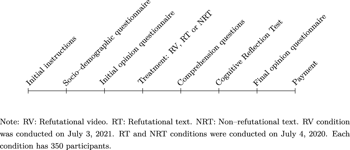
Fig. 1 Experiment procedure

Figure 1 depicts the steps of the experiment. First, participants see on their screens a consent form, where they are informed that the experiment is part of a research project in social sciences, that their personal data will be confidential, that their decisions will be anonymous, and that they will be paid if they agree to participate. If they do so, they are asked to sign the consent form. The next screen explains that they will be asked to complete several tasks, that if they complete all of them, they will receive a payment of six euros, and that one of the tasks will allow them to obtain two additional euros if they perform it correctly. They are also informed that the tasks will take about 20 minutes but they can use more time if they wish. Instructions emphasize that in the opinion questionnaires there are no correct or incorrect answers, and remind participants that payment does not depend on these answers, but on task completion (see the initial instructions in Appendix 5).

After a set of socio-demographic questions, participants fill out the questionnaire eliciting initial beliefs. On the next screen, participants see either the RT, the NRT, or the RV according to the condition they have been assigned to. They can take their time to read and re-read the texts, as they are not given a time limit. Participants in the video condition can also take their time and view the video several times if they wish, and they can also pause it.

After participants have read the texts or watched the video, we assess their attention and understanding of the content by showing a screen with two comprehension questions. These questions are shown in Appendix 2.5 and are the same across the three conditions. If participants answer both questions correctly, their payment increases by 2 euros. They cannot go back to previous screens with the text or the video to answer the questions. They are informed about this before being presented with the text or the video. Note that, through these two questions, we incentivize that participants pay attention to the texts or the video, as this is an essential aspect of the experiment. These are the only two questions that have a correct or an incorrect answer. We do not incentivize answers to all other questions and statements, since for them there are no correct or incorrect answers. We expect participants to answer in good faith by informing them, from the outset, that the study is part of a social research project carried out by professors from several universities, who will not be able to see or verify their personal identity, and that the purpose of the study is to contribute to a better understanding of our society by investigating people’s views. Moreover, since polls and studies are often used by policy-makers, participants in our study may have an intrinsic interest in revealing their true beliefs.

On the next screen participants answer an 8-item Cognitive Reflection Test. We adapt the original questions in Frederick (Reference Frederick2005), Toplak et al. (Reference Toplak, West and Stanovich2014), Thomson and Oppenheimer (Reference Thomson and Oppenheimer2016) to have economic content, so that they do not appear too disconnected from all other statements that have a socio-economic character. The eight items are shown in Appendix 4. We present them after the respective intervention to prevent the CRT from affecting participants’ reaction to the intervention.

Following the CRT questions, participants answer the final opinion questionnaire. In the closing screen participants are informed about the total payment and thanked for their collaboration. Appendix 5.2 shows all the instructions given to participants on each screen, which are the same across conditions.Footnote ¹⁵

3 Analysis

To test the hypotheses, we specify the following general regression:

(1)

\begin{matrix} y_{i} = α + β D_{i} + ε_{i} \end{matrix}

where $y_{i}$ is the change in beliefs, computed as the difference between a participant’s response to the statement on rent controls after the intervention and her response before the intervention. We transform the original responses in the five-point scale into numerical values as follows: 5 (totally disagree), 4 (disagree), 3 (do not know), 2 (agree), and 1 (totally agree). Hence $y_{i}$ takes values between $- 4$ (a change from fully disagree pre-intervention to fully agree post-intervention) and 4 (a change from fully agree pre-intervention to fully disagree post-intervention). That is, a positive value obtains when the response varies from agreement towards disagreement with the misconception. If the participant provides the same response in both questionnaires, the change is zero. $D_{i}$ is a dummy variable equal to one if the participant is exposed to a given treatment and zero otherwise.

To test for the first hypothesis we estimate Eq. (1) by comparing the change in beliefs of participants exposed to the RV relative to the change in beliefs of participants exposed to the RT, both unconditional and conditional to the initial belief. Hence $D_{i}$ is a dummy variable equal to one if the participant is exposed to the video and zero if she/he is exposed to the RT. Testing for H1 also involves estimating Eq. (1) by comparing the change in beliefs of participants exposed to the RV relative to the change in beliefs of participants exposed to the NRT, both unconditional and conditional to the initial belief. Hence $D_{i}$ in this case is a dummy variable equal to one if the participant is exposed to the video and zero if she/he is exposed to the NRT.

To test for the second hypothesis we estimate Eq. (1) by comparing the change in beliefs of participants exposed to the RT relative to the change in beliefs of participants exposed to the NRT, both unconditional and conditional to the initial belief. In this specification, $D_{i}$ is a dummy variable equal to one if the participant is exposed to the RT and zero if she/he is exposed to the NRT.

To test for the third hypothesis we build on the models above adding participants’ CRT scores to the regressions. To additionally assess whether the effect of the treatment varies with the propensity to think analytically, we add an interaction term between CRT score and the corresponding dummy variable.

Furthermore, we explore whether the change in beliefs is correlated with other personality traits, such as attentiveness, as captured by the time spent reading the texts or watching the video. We build on the models specified above with the CRT scores and add this attentiveness measure. We also study whether the effect of the interventions varies across gender, education level or housing ownership status by separately estimating the treatment effects in these subsamples.

4 Results

4.1 Descriptives

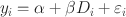
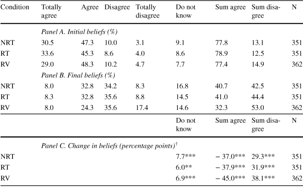
Table 1 reports the distribution of the degree of agreement with the statement about rent controls before and after each intervention. Figures 2 and 3 show the graphical description of these data. The distribution of initial beliefs is very similar in the three conditions: about 77 to 79% of participants agree or totally agree with the statement—that is, hold the misconception—while only 12 to 15% disagree (see Panel A in Table 1 and Fig. 2). These numbers are in line with findings from Brandts et al. (Reference Brandts, Busom, Lopez-Mayan and Panadés2022), where the misconception is initially shared by 75% to 84% of participants in the laboratory experiment, and by 70 to 78% in the field, depending on the condition. Note that these percentages are also similar to those found in polls conducted in Spain, Germany, in the UK or in the USA (see footnote 1).

Table 1 Prevalence of the misconception and change of beliefs

Condition	Totally agree	Agree	Disagree	Totally disagree	Do not know	Sum agree	Sum disagree	N
	Panel A. Initial beliefs (%)
NRT	30.5	47.3	10.0	3.1	9.1	77.8	13.1	351
RT	33.6	45.3	8.6	4.0	8.6	78.9	12.5	351
RV	29.0	48.3	10.2	4.7	7.7	77.4	14.9	362
	Panel B. Final beliefs (%)
NRT	8.0	32.8	34.2	8.3	16.8	40.7	42.5	351
RT	8.3	32.8	35.6	8.8	14.5	41.0	44.4	351
RV	8.0	24.3	35.6	17.4	14.6	32.3	53.0	362

		Do not know	Sum agree	Sum disagree	N
	Panel C. Change in beliefs (percentage points) $^{†}$
NRT		7.7***	− 37.0***	29.3***	351
RT		6.0**	− 37.9***	31.9***	351
RV		6.9***	− 45.0***	38.1***	362

NRT Non-refutational text. RT Refutational text. RV Refutational video. $^{†}$ Difference between percentage of participants answering a given level of agreement in the corresponding final and initial questionnaires. Significance levels of t-tests of the difference in means between final and initial questionnaires: * $p < 0.10$ , ** $p < 0.05$ , *** $p < 0.01$

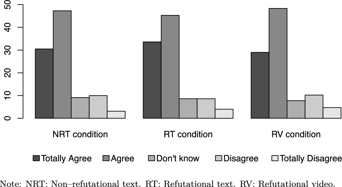
Fig. 2 Distribution of initial beliefs

After the treatment, the share of participants who disagree or totally disagree with the statement increases substantially in all three conditions, up to 42 to 53% depending on the treatment (see Panel B in Table 1 and Fig. 3). Note that the percentage in the case of the RV is over 10 percentage points (pp) higher than in the case of the NRT and over 8 pp higher than in the case of the RT. These percentages are substantially higher than those found in Brandts et al. (Reference Brandts, Busom, Lopez-Mayan and Panadés2022), where the share of the participants who disagree or totally disagree after the treatment ranges from 25% to 32% in the laboratory and from 10% to 29% in the field, depending on the condition. Nevertheless, the comparison of the distribution of final beliefs here with those in our previous work should be used with caution since the information treatments are different as well as the subject pool, as explained above.

Fig. 3 Distribution of final beliefs

Panel C in Table 1 shows the change in beliefs and the significance level from a test of difference in means. In both text conditions the percentage agreeing falls substantially, by about 37 pp, a drop of almost 50%. In the RV condition, the drop in the percentage of those who agree is more dramatic, being equal to 45 pp, almost 60%. These are the participants who abandon the misconception. Some of them move towards “don’t know” but most move towards disagreeing. In the NRT condition the share of those disagreeing increases by 29 pp, which is more than twofold the initial share. In the RT condition, the share disagreeing increases slightly more, by 32 pp. The percentage of those disagreeing in the RV condition increases by 38 pp, even more. All these changes are statistically significant.

According to these findings, the on-line intervention with shorter texts appears to be more successful in reducing the prevalence of the misconception than the interventions with the longer texts in Brandts et al. (Reference Brandts, Busom, Lopez-Mayan and Panadés2022), although one needs to take into account the change of subject pool and the fact that the current experiment was conducted online. More importantly, a visual presentation of the refutation arguments is, on a descriptive level, more effective than a text-only correction, be it the NRT or the RT.

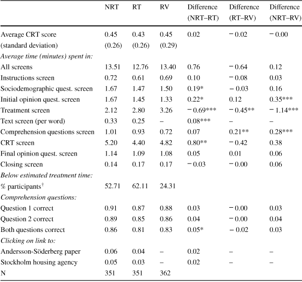
Table 2 shows a number of performance indicators: CRT scores and average time spent on each screen of the experiment. We do not observe significant differences for most of them across the three conditions. The CRT score is measured as the percentage of correct answers to the eight items included in the test. The mean score is around 0.45, in line with the average CRT score in Brandts et al. (Reference Brandts, Busom, Lopez-Mayan and Panadés2022) and in Mosleh et al. (Reference Mosleh, Pennycook, Arechar and Rand2021). To explore whether the CRT is correlated with initial beliefs, we regress the latter on the CRT and socio-demographic variables. Results are shown in Table 15 in Appendix 3. The CRT score is not significantly correlated with the initial belief in any of the conditions, which indicates that being more analytical is not associated to a lower prevalence of the misconception.

On average, participants spend around 13 minutes to complete all screens. This is lower than the expected duration of about 20 minutes, calculated on the basis of the length of the questionnaires, the video duration and the texts’ estimated read time (see Table 11). Time spent on the treatment screen exhibits significant differences across conditions, as expected, since the estimated duration of the treatments is somewhat different. Participants spend more time on the RT than on the NRT. Average time spent on the RT screen is 2.8 minutes, slightly below the estimated read time (3.4 minutes). Average time on the NRT screen is about equal to the estimated time of 2 minutes. Looking at time per word, however, we find that the RT is read faster than the NRT. Participants spend more time on the video than on the two texts, as average time on the RV screen is 3.26 minutes, which is higher than the video duration (2.42 minutes). We also observe that the percentage of participants who spend less than the estimated time on the treatment screen is substantially lower in the RV than in the text conditions. All this suggests that the RV increases the attention paid to the message, while texts are read more lightly.

Time spent on the comprehension question screen is significantly lower in the RV than in the two text conditions, with no significant difference between the last two. A possible interpretation is that participants focus more on the visual presentation, which allows them to respond faster to the comprehension questions. However, we do not observe large differences across conditions in the percentage of participants who answer both questions correctly. Finally, very few participants (about 5%) show an interest in checking the links to the Andersson-Söderberg paper or to the Stockholm housing agency website in the text-only corrections. Table 13 in Appendix 3 shows more statistics on the total time spent in the experiment and on each screen in the three conditions.

Table 2 Participants’ performance indicators

	NRT	RT	RV	Difference	Difference	Difference
				(NRT–RT)	(RT–RV)	(NRT–RV)
Average CRT score	0.45	0.43	0.45	0.02	$-$ 0.02	$-$ 0.00
(standard deviation)	(0.26)	(0.26)	(0.29)
Average time (minutes) spent in:
All screens	13.51	12.76	13.40	0.76	$-$ 0.64	0.12
Instructions screen	0.72	0.61	0.69	0.10	$-$ 0.08	0.03
Sociodemographic quest. screen	1.67	1.47	1.50	0.19*	− 0.03	0.16
Initial opinion quest. screen	1.67	1.45	1.33	0.22*	0.12	0.35***
Treatment screen	2.12	2.80	3.26	$-$ 0.69***	$-$ 0.45**	$-$ 1.14***
Text screen (per word)	0.33	0.25	–	0.08***	–	–
Comprehension questions screen	1.01	0.93	0.72	0.07	0.21**	0.28***
CRT screen	5.20	4.40	4.82	0.80**	$-$ 0.42	0.38
Final opinion quest. screen	1.14	1.09	1.08	0.05	0.01	0.06
Closing screen	0.14	0.17	0.17	$-$ 0.03	$-$ 0.00	0.06
Below estimated treatment time:
% participants $^{†}$	52.71	62.11	24.31
Comprehension questions:
Question 1 correct	0.91	0.87	0.88	0.03	$-$ 0.00	0.03
Question 2 correct	0.89	0.85	0.86	0.04	$-$ 0.00	0.04
Both questions correct	0.86	0.81	0.83	0.05*	− 0.02	0.03
Clicking on link to:
Andersson-Söderberg paper	0.06	0.04	–	0.02	–	–
Stockholm housing agency	0.05	0.03	–	0.02	–	–
N	351	351	362

NRT Non-refutational text. RT Refutational text. RV Refutational video. CRT Cognitive Reflection Test. CRT takes values between 0 and 1; it is computed as the percentage of correct answers to the eight questions included in the test. Significance levels of t-tests of the difference in means: * $p < 0.10$ , ** $p < 0.05$ , *** $p < 0.01$ . $^{†}$ % of participants spending less than the estimated time in the treatment screen: less than 2 minutes in the NRT and 3.4 minutes in the RT (as shown in Table 11); less than 2.42 minutes in the RV

4.2 Estimation results

The results shown in Tables 3 and 4 address the three research hypotheses formulated in Sect. 2.1.

Table 3 presents the estimation results of the differential impact of the treatments on participants’ beliefs, comparing pairwise and pooling all three treatments. We first estimate Eq. (1) with and without the set of socio-demographic variables in each case to assess the sensitivity of the results to the observed sample unbalances across conditions discussed above. Since there are no large differences in the estimated treatment effects once we have accounted for socio-demographics, we focus on commenting on the results with controls (Table 14 in Appendix 3 shows the estimated coefficients of the control variables).

Table 3 Estimated treatment effects on revising the misconception

	RV vs. RT			RT vs. NRT			RV vs. NRT			Pooled $^{†}$
	(1)	(2)	(3)	(4)	(5)	(6)	(7)	(8)	(9)	(10)	(11)	(12)
RV	0.17	0.18*	0.17	–	–	–	0.23**	0.26***	0.26***	0.17	0.19*	0.18*
RV	(0.10)	(0.11)	(0.11)				(0.10)	(0.10)	(0.10)	(0.10)	(0.10)	(0.10)
RT	–	–	–	0.06	0.07	0.08	–	–	–	–	–	–
RT				(0.10)	(0.10)	(0.10)
NRT	–	–	–	–	–	–	–	–	–	$-$ 0.06	$-$ 0.07	$-$ 0.08
NRT										(0.10)	(0.10)	(0.10)
CRT	–	–	0.48**	–	–	0.51***	–	–	0.45**	–	–	0.51***
CRT			(0.20)			(0.20)			(0.19)			(0.16)
Controls	No	Yes	Yes	No	Yes	Yes	No	Yes	Yes	No	Yes	Yes
N	713	713	713	702	702	702	713	713	713	1064	1064	1064
$R^{2}$	0.00	0.07	0.08	0.00	0.06	0.07	0.01	0.05	0.06	0.01	0.05	0.06

Dependent variable: belief change after intervention; it takes values between $- 4$ and 4 (positive values indicate a change away from the misconception). NRT Non-refutational text. RT Refutational text. RV Refutational video. Pooled $^{†}$ : pooled sample with all three conditions. Robust standard errors in parentheses. Significance levels: * $p < 0.10$ , ** $p < 0.05$ , *** $p < 0.01$ . See the set of control variables in Table 14 in Appendix 3

Column (2) shows that the RV reduces the misconception relative to the RT—as the positive coefficient indicates a change away from the misconception—at the 10% significance level. The effect size, as measured by the ratio of the estimated coefficient to the standard deviation of the dependent variable indicates that the video induces a revision in beliefs towards disagreeing with the statement by 0.13 standard deviations. Column (5) shows that the RT has a positive but not significant impact on reducing the prevalence of the misconception relative to the NRT. Since both RT and NRT decrease the prevalence of the misconception by a similar magnitude (Table 1), the additional effect of the RT is of small size and not precisely identified. Column (8) shows that the effect of the RV with respect to the NRT is larger and significant at the 1% level. The effect size is of 0.20 standard deviations, larger than the effect with respect to the RT. When pooling all three conditions in column (11), the estimated effects of the RV and the NRT with respect to the RT—the base category—are very close to those in columns (2) and (5). Since results are robust to conducting the pooled and pairwise estimations, we use the latter in the rest of the paper, as sample sizes are sufficiently large. This approach is more flexible than pooling because it allows the coefficients of control variables to vary across pairwise comparisons. Pooling all conditions constrains the coefficients of control variables to be equal and, therefore, any difference in participants’ distribution of characteristics across conditions would be captured by the treatment coefficients.

Columns (3), (6), (9) and (12) show that adding the CRT score to each specification with controls barely changes the treatment estimates. In all pairwise comparisons a higher CRT score is significant and associated with a stronger change away from the misconception, with very little variation across conditions. The estimates range between 0.45 in the RV vs NRT comparison and 0.51 in the RT vs NRT comparison, implying an effect size of 0.34 to 0.40 standard deviations. Recall that the CRT score is not significantly correlated with the initial belief in any of the conditions, as shown above. However, being more analytical does predict the ability to revise the misconception.

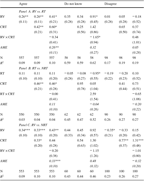
Results in Table 3 capture the overall effects of treatments on changing beliefs. These overall effects, however, may conceal differences across the distribution of initial beliefs. We thus estimate Eq. (1) separately for the groups of participants who initially agree, don’t know and disagree with the statement.Footnote ¹⁶ Table 4 contains the results for the specifications with all the controls. This table also shows the results from the specifications that add the CRT score and its interaction with the treatment.

In Panel A we compare the RV to the RT. The RV has a positive and significant effect at 5% level on abandoning the misconception of those participants who initially agree with it, with a coefficient of 0.26 and an effect size of 0.21 standard deviations. The effect is positive although not significant for the other two initial belief categories. Adding the CRT does not alter these patterns. The CRT score is positively correlated to abandoning the misconception (equivalent to 0.34 standard deviations) but the association is only significant for those who initially agree. Adding an interaction term between the RV and the CRT score does not change previous results, as shown by the estimated average marginal effect (AME), which is 0.26 in both regressions. That is, the effect of the RV does not vary with CRT scores.

In sum, the RV improves on the RT basically through the effect on those who initially agree with the misconception. Note that participants who initially disagree or those who are uncertain do not significantly react to the RV. Therefore, the RV induces a reduction of the misconception by shifting the whole distribution of beliefs towards disagreeing.

In Panel B we compare the RT to the NRT. We do not find significant differential effects of the RT along the distribution of initial beliefs. As in Panel A, higher CRT scores are associated with a higher abandonment of the misconception, with the correlation being slightly stronger (0.40 standard deviations). The interaction term between the RT and the CRT score is not significant, as above. These results are qualitatively in line with those obtained in the laboratory in Brandts et al. (Reference Brandts, Busom, Lopez-Mayan and Panadés2022).

Panel C in Table 4 shows the comparison between the RV and the NRT. Here, as in Panel A, the RV has a positive effect on revising the misconception of those who initially hold it. The effect is significant at 1% level and its size is equivalent to 0.28 standard deviations, stronger than the effect with respect to the RT in Panel A. The CRT score also shows a positive correlation with moving away from the misconception. The interaction term between the CRT score and the treatment is not significant.

Hence, our results indicate that the ranking in terms of effectiveness in dispelling the misconception is the RV, followed by the RT and, last, the NRT.Footnote ¹⁷ They also show that the importance of the association between the disposition to reflective thinking and the revision of the belief slightly decreases when information is presented in video instead of in text.

Table 4 Estimated treatment effects on revising the misconception, conditional on initial belief

	Agree			Do not know			Disagree
	Panel A. RV vs. RT
RV	0.26**	0.26**	0.41*	0.35	0.34	0.91*	0.01	0.05	$-$ 0.18
RV	(0.11)	(0.11)	(0.21)	(0.28)	(0.28)	(0.45)	(0.28)	(0.28)	(0.52)
CRT		0.42**	0.60*		0.25	1.42		0.65	0.37
CRT		(0.21)	(0.31)		(0.56)	(0.86)		(0.50)	(0.74)
RV $\times$ CRT			$-$ 0.34			$-$ 1.65*			0.48
RV $\times$ CRT			(0.41)			(0.94)			(1.01)
AME			0.26**			0.32			0.05
AME			(0.11)			(0.27)			(0.28)
N	557	557	557	58	58	58	98	98	98
$R^{2}$	0.09	0.09	0.10	0.59	0.59	0.62	0.17	0.19	0.19
	Panel B. RT vs. NRT
RT	0.11	0.11	0.11	$-$ 0.05	$-$ 0.08	$-$ 0.95*	$-$ 0.19	$-$ 0.20	0.10
RT	(0.10)	(0.10)	(0.20)	(0.28)	(0.27)	(0.55)	(0.22)	(0.23)	(0.52)
CRT		0.46**	0.46*		0.95	0.05		0.41	0.73
CRT		(0.21)	(0.28)		(0.78)	(1.04)		(0.44)	(0.51)
RT $\times$ CRT			$-$ 0.00			2.59			$-$ 0.65
RT $\times$ CRT			(0.41)			(1.54)			(1.08)
AME			0.11			$-$ 0.04			$-$ 0.20
AME			(0.10)			(0.26)			(0.22)
N	550	550	550	62	62	62	90	90	90
$R^{2}$	0.03	0.04	0.04	0.45	0.47	0.52	0.26	0.27	0.27
	Panel C. RV vs. NRT
RV	0.34***	0.33***	0.43**	0.44	0.45	0.92	$-$ 0.35*	$-$ 0.33	0.15
RV	(0.10)	(0.10)	(0.20)	(0.33)	(0.34)	(0.57)	(0.21)	(0.20)	(0.42)
CRT		0.33*	0.44		0.54	1.30		0.77**	1.31***
CRT		(0.20)	(0.28)		(0.63)	(1.02)		(0.37)	(0.48)
RV $\times$ CRT			$-$ 0.20			$-$ 1.15			$-$ 1.01
RV $\times$ CRT			(0.38)			(1.26)			(0.80)
AME			0.33***			0.48			$-$ 0.32
AME			(0.10)			(0.32)			(0.20)
N	553	553	553	60	60	60	100	100	100
$R^{2}$	0.09	0.10	0.10	0.43	0.44	0.46	0.23	0.26	0.27

Dependent variable: belief change after intervention; it takes values between $- 4$ and 4 (positive values indicate a change away from the misconception). RT Refutational text. NRT Non-refutational text. RV Refutational video. Robust standard errors in parentheses. Significance levels: * $p < 0.10$ , ** $p < 0.05$ , *** $p < 0.01$ . All regressions include the same control variables as in Table 3. AME Average marginal effect of the treatment

To sum up, our empirical findings provide the following evidence regarding the three research hypotheses as follows:

Result 1. “The RV has a significantly higher impact on abandoning the misconception than the RT, and even higher impact relative to the NRT. In both cases the effect of the RV is driven by the impact on participants who initially hold the misconception.”

Our results support H1. Visual communication is more effective in dispelling the misconception than refuting it through a written text, even if the text is refutational.

Result 2. “The RT is not significantly more effective than the NRT in dispelling the misconception.”

Our estimates do not support H2. Although the effect of a written RT is positive, it is small, and its differential impact with respect to the NRT is not precisely estimated. The refutational elements of the RT do not seem to stand out among the other sentences. This result concurs with Brandts et al. (Reference Brandts, Busom, Lopez-Mayan and Panadés2022). Note, however, that in that study the proportion of participants who hold the misconception after the intervention is of about 54 to 63%; while here this percentage is smaller, 41%. The drop is now of 37 pp, almost double than in the former study. This suggests that short texts are more effective than long texts.

Result 3. “A higher propensity to reflective thinking significantly induces a change away from the misconception in all treatments for participants who initially hold it.”

Our findings show a positive association between the CRT score and the change away from the misconception, especially for the key group of interest, i.e., participants who initially have the misconception. This evidence is in line with H3. However, we should be cautious when drawing conclusions about H3. Since CRT scores are collected after the treatment in each condition for the reason discussed above, the refutational correction or the visual elements may affect CRT scores. Results suggest that this potential influence is not serious since the average CRT score is not significantly different across the three conditions, as shown in Table 2. Nevertheless, we cannot fully disregard that the treatments may affect the answers to the CRT questionnaire and, thus, we have to be cautious about the causal effect of the propensity thinking on the change of beliefs. Finally, we do not find evidence that the treatment effect varies with the CRT score.

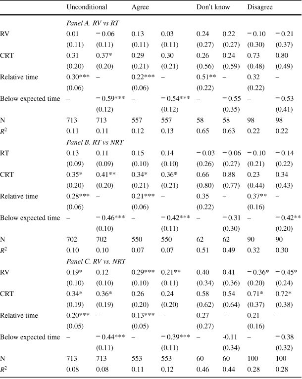
We explore whether the mechanism that makes the RV more effective than written information is related to a higher ability of the RV to capture and keep the viewer’s attention. As described above, in the case of the NRT condition 53% of participants spend less time than expected on the text screen; in the RT condition, 62% are below expected time. In the RV condition, in contrast, only 24% spend less time than the whole video duration. This suggests that the video attracts and keeps the attention of more participants than the text interventions. To analyze the role of attention, we define two alternative measures. One is the ratio between the time spent on the treatment screen by an individual and the expected time to be spent on that screen. This is 2:42 minutes in the case of the RV, and 3:40 minutes in the RT, and 2:00 minutes in the NRT (see Sect. 2.2). The second measure is a dummy variable equal to one if time spent on the treatment screen is below the expected time and zero otherwise.

We separately add these two measures to the specification with the CRT and the controls both for the full sample and conditional on initial beliefs. Table 5 shows that the estimated CRT and treatment effects are robust to the attention measure used. Relative time has always a positive effect on revising beliefs, and the indicator for time below the expected time shows a congruent negative sign. Estimated treatment effects fall somewhat compared to those in Tables 3 and 4, as does the effect of the CRT. This suggests that part of the positive effect of the video found above can be attributed to the video per se prompting higher attention compared to plain text. In other words, if participants paid as much attention to the text as they do to the video, the impact of the two formats would likely be similar. When comparing the RV with the NRT, the impact of attention is significant and positive, and so does the treatment effect. Overall, these results suggest that integrating visual elements increases attention and thus comprehension of the arguments and evidence presented in the correction, boosting the refutational elements.

Table 5 Estimated treatment effects adding attention measures

	Unconditional		Agree		Don’t know		Disagree
	Panel A. RV vs RT
RV	0.01	$-$ 0.06	0.13	0.03	0.24	0.22	$-$ 0.10	$-$ 0.21
RV	(0.11)	(0.11)	(0.11)	(0.11)	(0.27)	(0.27)	(0.30)	(0.37)
CRT	0.31	0.37*	0.29	0.30	0.26	0.24	0.73	0.80
CRT	(0.20)	(0.20)	(0.21)	(0.21)	(0.56)	(0.59)	(0.48)	(0.49)
Relative time	0.30***	–	0.22***	–	0.51**	–	0.32	–
Relative time	(0.06)		(0.06)		(0.22)		(0.22)
Below expected time	–	$-$ 0.59***	–	$-$ 0.54***	–	$-$ 0.55	–	$-$ 0.53
Below expected time		(0.12)		(0.12)		(0.35)		(0.41)
N	713	713	557	557	58	58	98	98
$R^{2}$	0.11	0.11	0.12	0.13	0.65	0.63	0.22	0.22
	Panel B. RT vs NRT
RT	0.13	0.11	0.15	0.14	$-$ 0.03	$-$ 0.06	$-$ 0.10	$-$ 0.14
RT	(0.09)	(0.09)	(0.10)	(0.10)	(0.26)	(0.27)	(0.21)	(0.22)
CRT	0.35*	0.41**	0.34*	0.36*	0.66	0.88	0.23	0.34
CRT	(0.20)	(0.20)	(0.21)	(0.21)	(0.80)	(0.77)	(0.44)	(0.43)
Relative time	0.28***	–	0.21***	–	0.35	–	0.37**	–
Relative time	(0.06)		(0.06)		(0.22)		(0.16)
Below expected time	–	$-$ 0.46***	–	$-$ 0.42***	–	$-$ 0.31	–	$-$ 0.42**
Below expected time		(0.10)		(0.11)		(0.30)		(0.20)
N	702	702	550	550	62	62	90	90
$R^{2}$	0.10	0.10	0.07	0.07	0.51	0.49	0.32	0.30
	Panel C. RV vs. NRT
RV	0.19*	0.12	0.29***	0.21**	0.40	0.41	$-$ 0.36*	$-$ 0.45*
RV	(0.10)	(0.10)	(0.10)	(0.11)	(0.34)	(0.36)	(0.20)	(0.24)
CRT	0.34*	0.36*	0.26	0.24	0.58	0.54	0.71*	0.72*
CRT	(0.19)	(0.19)	(0.20)	(0.20)	(0.62)	(0.64)	(0.37)	(0.38)
Relative time	0.20***	–	0.13***	–	0.27	–	0.21	–
Relative time	(0.05)		(0.05)		(0.27)		(0.16)
Below expected time	–	$-$ 0.44***	–	$-$ 0.39***	–	-0.11	–	$-$ 0.38
Below expected time		(0.11)		(0.11)		(0.34)		(0.32)
N	713	713	553	553	60	60	100	100
$R^{2}$	0.08	0.08	0.11	0.12	0.46	0.44	0.28	0.28

Dependent variable: belief change after intervention; it takes values between $- 4$ and 4 (positive values indicate a change away from the misconception). RT Refutational text. NRT Non-refutational text. RV Refutational video. Relative time: ratio between the time spent on the treatment screen and the expected time to be spent on that screen. Below expected time: dummy variable equal to 1 if time spent on the treatment screen is below the expected time and 0 otherwise. Robust standard errors in parentheses. Significance levels: * $p < 0.10$ , ** $p < 0.05$ , *** $p < 0.01$ . All regressions include the same control variables as in Table 3

4.3 Additional results

We explore whether treatment effects vary across several socio-demographic characteristics and according to several measures of trust. We focus on the subsample of participants who initially hold the misconception (agree with the statement) because this is where the relevant changes take place as discussed above.

We first split the sample of participants according to whether they are tenants or owners. Tenants and owners might differ in their reaction to a treatment, since they would be potentially affected in opposite directions by rent regulation. Perhaps current tenants, whose interest is to pay low rents, stick to their initial belief more than owners, who may be more receptive to the intervention, given that they may wish to rent out at some point. Panel A in Table 6 shows, however, that the treatments do not significantly differ for tenants and owners. Note that sample size is small in the case of tenants, which reduces the precision of the estimates. The only exception is for the RV vs NRT comparison, where the positive impact of the RV on owners’ revision is significant. This is in line with owners being more receptive to the intervention than tenants, who are not significantly affected by it.

Men and women often differ in their attitudes or behavior. In our data gender is significantly correlated with the initial opinion (see Table 15 in Appendix 3). Results in Panel B, Table 6 show some differences in the effect of treatment on beliefs across gender but there is no clear pattern. For the RV vs RT comparison, RV is significant for men but not for women and for the RT vs NRT comparison, RT is significant for women but not for men. For the RV vs NRT comparison, both men and women significantly revise their beliefs but the video has a stronger effect on women.

Education is not significantly correlated with the initial belief (see Table 15 in Appendix 3) but more educated individuals may react differently to the treatments than less educated ones. To study this we split the sample into low and highly educated participants. Highly educated includes those who report tertiary education as their maximum schooling level as well as participants who report being currently enrolled in tertiary education. Results in Panel C of Table 6 show that the video is more effective for the highly than for the low educated participants, relative to both the RT and NRT. When comparing the two text conditions the effects are not significant for any education level. Therefore, results suggest that participants with high education are more likely to abandon the misconception after watching the video than participants with low education.

Table 6 Heterogeneous effects conditional on initially agreeing with rent controls (I)

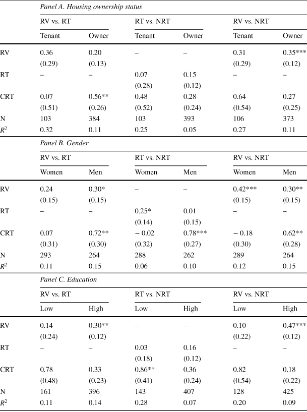
	Panel A. Housing ownership status
	RV vs. RT		RT vs. NRT		RV vs. NRT
	Tenant	Owner	Tenant	Owner	Tenant	Owner
RV	0.36	0.20	–	–	0.31	0.35***
RV	(0.29)	(0.13)			(0.29)	(0.12)
RT	–	–	0.07	0.15	–	–
RT			(0.28)	(0.12)
CRT	0.07	0.56**	0.48	0.28	0.64	0.27
CRT	(0.51)	(0.26)	(0.52)	(0.24)	(0.54)	(0.25)
N	103	384	103	393	106	373
$R^{2}$	0.32	0.11	0.25	0.05	0.27	0.11

	Panel B. Gender
	RV vs. RT		RT vs. NRT		RV vs. NRT
	Women	Men	Women	Men	Women	Men
RV	0.24	0.30*	–	–	0.42***	0.30**
RV	(0.15)	(0.15)			(0.15)	(0.15)
RT	–	–	0.25*	0.01	–	–
RT			(0.14)	(0.15)
CRT	0.07	0.72**	− 0.02	0.78***	− 0.18	0.62**
CRT	(0.31)	(0.30)	(0.32)	(0.27)	(0.30)	(0.28)
N	293	264	288	262	289	264
$R^{2}$	0.11	0.15	0.06	0.10	0.12	0.15

	Panel C. Education
	RV vs. RT		RT vs. NRT		RV vs. NRT
	Low	High	Low	High	Low	High
RV	0.14	0.30**	–	–	0.10	0.47***
RV	(0.24)	(0.12)			(0.22)	(0.12)
RT	–	–	0.03	0.16	–	–
RT			(0.18)	(0.12)
CRT	0.78	0.33	0.86**	0.36	0.82	0.18
CRT	(0.48)	(0.23)	(0.41)	(0.24)	(0.54)	(0.22)
N	161	396	143	407	128	425
$R^{2}$	0.11	0.14	0.28	0.07	0.20	0.09

We finally explore whether participants react differently to the treatments depending on their degree of trust towards economic statistical information, and towards several information sources. We use the questions on trust that participants answer before the treatments: what they consider to be the most trustworthy source for economic and social information, and the extent to which they mistrust economic statistics. Table 7 shows the distribution of responses for these two questions. The distributions are similar across conditions and show, maybe surprisingly, that around 70% of participants select politicians as the most trustworthy source for economic and social information. More than half of the participants show mistrust towards economic statistics: they agree or totally agree that economic statistics do not reflect, in general, the true economic situation.

Table 7 Distribution of responses to statements on trust

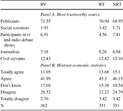
	RV	RT	NRT
	Panel A. Most trustworthy source
Politicians	71.55	70.94	68.95
Social scientists	1.93	3.42	1.71
Participants in tv and radio debate shows	6.91	4.56	7.41
Journalists	7.18	8.26	6.84
Civil servants	12.43	12.82	15.10
	Panel B. Mistrust economic statistics
Totally agree	11.05	13.68	15.1
Agree	41.99	45.3	46.15
Don’t know	17.68	15.38	10.54
Disagree	26.52	22.22	24.79
Totally disagree	2.76	3.42	3.42
N	362	351	351

RT Refutational text. NRT Non-refutational text. RV Refutational video. Trustworthy information source: “Of the following options, indicate your most trustworthy source for social and economic information: a) participants in radio and tv debate shows; b) politicians; c) civil servants; d) social scientists who work at universities; d) journalists”. Mistrust statistics statement: “Economic statistics do not reflect, in general, the true economic situation”

Panel A in Table 8 shows the results from separate regressions run after splitting the sample according to whether participants consider politicians or other sources to be the most trustworthy source for economic and social information. In the comparison between visual and text-only messages (RT or NRT), participants who trust other sources significantly abandon the misconception, while those who trust politicians, only significantly update their beliefs if they receive the video compared with receiving the NRT. In the comparison between RT and NRT, the effects are not significant. Although the evidence is not very strong, these results suggest that the visual message is somewhat more effective for those who declare that politicians are not their most trustworthy source.

Panel B in Table 8 presents the regression results for the treatment comparisons after splitting the sample according to whether participants mistrust economic statistics, i.e., those who respond “totally agree” or “agree” to the statement. Those who mistrust statistics (columns Yes in the table) are more convinced by the RV both when compared to the RT and to the NRT. In the latter comparison (RV vs NRT), the video is also effective for those who do not mistrust statistics. The comparison between the text-only messages (RT vs NRT) shows that the RT only has a significant positive effect on the group who trust economic statistics. These results suggest that the visual message is a especially effective format for those who do not trust economic data.

Table 8 Heterogeneous effects conditional on initially agreeing with rent controls (II)

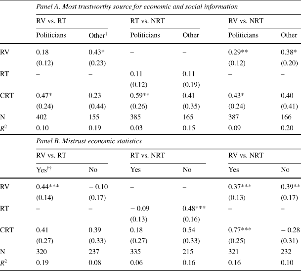
	Panel A. Most trustworthy source for economic and social information
	RV vs. RT		RT vs. NRT		RV vs. NRT
	Politicians	Other $^{†}$	Politicians	Other	Politicians	Other
RV	0.18	0.43*	–	–	0.29**	0.38*
RV	(0.12)	(0.23)			(0.12)	(0.20)
RT	–	–	0.11	0.11	–	–
RT			(0.12)	(0.19)
CRT	0.47*	0.23	0.59**	0.41	0.43*	0.40
CRT	(0.24)	(0.44)	(0.26)	(0.35)	(0.24)	(0.41)
N	402	155	385	165	387	166
$R^{2}$	0.10	0.19	0.03	0.15	0.09	0.20

	Panel B. Mistrust economic statistics
	RV vs. RT		RT vs. NRT		RV vs. NRT
	Yes $^{† †}$	No	Yes	No	Yes	No
RV	0.44***	− 0.10	–	–	0.37***	0.39**
	(0.14)	(0.17)			(0.13)	(0.17)
RT	–	–	− 0.09	0.48***	–	–
			(0.13)	(0.16)
CRT	0.41	0.39	0.18	0.54	0.77***	− 0.28
	(0.27)	(0.33)	(0.27)	(0.33)	(0.25)	(0.31)
N	320	237	335	215	321	232
$R^{2}$	0.19	0.08	0.06	0.16	0.16	0.10

Dependent variable: belief change after intervention; it takes values between $- 4$ and 4 (positive values indicate a change away from the misconception). RT: Refutational text. NRT: Non-refutational text. RV: Refutational video. Robust standard errors in parentheses. Significance levels: * $p < 0.10$ , ** $p < 0.05$ , *** $p < 0.01$ . All regressions include the same control variables as in Table 3. $^{†}$ Other: it includes the other possible answers to the question on the most trustworthy information source (participants in radio and tv debate shows; civil servants; social scientists who work at universities; and journalists), see Appendix 1. $^{† †}$ Yes: participants’ answer to the Mistrust statistics statement is “totally agree” or “agree”. No: participants’ answer to the Mistrust statistics statement is “totally disagree”, “disagree” or “don’t know” (see Appendix 1)

5 Conclusions

The accumulation of research about the causes and effects of socio-economic phenomena has contributed to building a strong consensus among researchers on some issues. A case in point are the effects of rent controls on rental housing availability. Yet, this consensus has not reached a majority of citizens, who endorse and demand this policy in the hope that it will have positive effects on access to housing. Effective communication between researchers and the public faces several barriers in all fields of knowledge. Some stem from the inherent difficulty involved in explaining concepts, methods and results in a simple way without losing accuracy; others may arise from different biases and values that arise when lay people process information. Barriers may be stronger in the case of social sciences, where even providing hard factual information encounters skepticism (Nyhan, Reference Nyhan2020). The concern about the serious consequences that ignoring solid knowledge may have, has led to the emergence of a body of research on how to communicate science to policymakers and the public in several fields. This concern is further justified by the rise of mis-information in the media and social networks.

In this paper we have investigated the effectiveness of specific communication formats in confronting the widespread belief that rent control increases affordable housing using a sample of ordinary citizens. We design a short video that combines a refutational approach with images and we test its effectiveness relative to short text-only messages. The video contributes to closing the gap between scientific consensus and public opinion substantially. Indeed, while 77% of participants initially hold the misconception, after the refutational video intervention this percentage drops to 32%, that is, by 45 pp. This is an additional 12 pp compared to the effect of texts that convey the same information but with words only. The estimated effect of the visual message is significant and induces an abandonment of the misconception for participants who initially hold it. Our results suggest that part of this positive effect may be driven by the higher attention that the video attracts. We interpret that visual communication, by reducing cognitive effort, makes economic arguments easier to grasp. Our results are in line with previous literature that finds that visual tools are more effective than text-only messages to dispel misconceptions about other topics (Mayer & Moreno, Reference Mayer and Moreno2003; Goldberg et al., Reference Goldberg, van der Linden, Ballew, Rosenthal, Gustafson and Leiserowitz2019; Young et al., Reference Young, Jamieson, Poulsen and Goldring2018; Reynolds et al., Reference Reynolds, Pilling and Marteau2018).

Our results also show that short texts are more effective than longer ones. Both short RT and NRT lead to an additional 15 percentage points reduction in the prevalence of the misconception, compared to the reduction in Brandts et al. (Reference Brandts, Busom, Lopez-Mayan and Panadés2022), where texts are twice as long. Nonetheless, like in our previous work, the refutational correction in a written message does not improve on a non-refutational one. We wish to emphasize that the positive effects of the video and short texts are obtained with a pool of ordinary citizens who are the natural target for communicating economic policies.

The main takeaway from this study is that communicating to the general public evidence about the effects of rent control in a visual refutational format goes a long way in dispelling this misconception. Citizens are currently highly exposed to visual communication in the media; there is also a lot of competition for their attention. We therefore believe that it is important that the format that uses images is the most successful in our case. A practical implication is that researchers should rely more on visual refutational elements to communicate research findings to the public. Academic associations, for instance, could design and disseminate refutational videos addressing misconceptions about socio-economic issues. Our study, thus, adds to the still scarce research in economics on the effectiveness of different modes of communicating research findings that confront popular beliefs. We show that our approach, refutational visual communication, may be a promising method to communicate other counter-intuitive economic findings to ordinary citizens. We also add to the literature on misconceptions in political and economic psychology, and, more broadly, to the literature on science communication.

Yet, in our experiment 32% of participants still hold the misconception after the refutational video intervention. Although obviously one cannot expect to persuade everybody, we think that this is still a high percentage, given the high consensus among researchers. We see several possibilities that remain to be explored in future research. The first pertains to the characteristics of our refutational video. In designing it we have been quite restricted, since we needed to make it very parallel to the refutational text to properly identify the effect of the pure visual element. A richer, less restricted video could be more effective, closing the gap further.

Second, our communication strategy may be improved by adding some other important aspects. The standard refutation correction is based on inducing people to approach the issue at hand analytically. One possible reason that may be behind the resistance to move away from the misconception is that corrections involving topics sensitive to political views or worldviews are perceived as a threat to individuals’ social identity. This kind of misconceptions may be harder to debunk, and may require the refutation approach to account for this explicitly. Other issues that warrant further research are for how long changes in beliefs persist, whether peer-to-peer communication would affect them (Hüning et al., Reference Hüning, Mechtenberg and Wang2021), and whether changes in beliefs are related to ideology. Moreover, a relevant question for further research is whether changes in beliefs translate into behavior such as voting decisions. Our purpose here is to put the focus on whether communication formats have an impact. We think that this is the first battle, so to speak, we, as economists, have to fight.

A final issue is whether and how the source of information may affect the reaction to information treatments. Regarding the subject of rent-control, the reaction might be different depending on whether the information is provided by political parties, civic associations or experts. Ecker et al. (Reference Ecker, Lewandowsky, Cook, Schmid, Fazio, Brashier, Kendeou, Vraga and Amazeen2022) review the psychological drivers of misinformation belief and its resistance to correction and also refer to the issue of which societal players have the power to affect public perceptions. This is an important subject in relation to misconceptions about rent control and other policies that should be studied in the future.

Funding

Open Access funding provided thanks to the CRUE-CSIC agreement with Springer Nature.

Appendices

Appendix 1: The statements

Participants show their degree of agreement using a 5-point Likert scale displayed on each screen after the corresponding statement: totally disagree, disagree, don’t know, disagree, totally disagree (Table 9).

• Rent control:

Establishing rent controls, such that rents did not exceed a certain amount of money, would increase the number of people who have access to housing facilities.
• Online platforms for vacation rentals:

Online platforms for renting vacation apartments, like Airbnb or Wimdu, are one of the main cause of the rising rents.
• Housing investment funds:

Housing investment funds own most of the housing for rent.
• Affordable housing:

Government should guarantee that everybody can buy a house.
• Mistrust statistics:

Economic statistics do not reflect, in general, the true economic situation.
• Trustworthy information source:

Of the following options, indicate your most trustworthy source for social and economic information: a) participants in radio and tv debate shows; b) politicians; c) civil servants; d) social scientists who work at universities; d) journalists.
• Disagreement among scientists:

Disagreement among scientists on some topics shows that science reflects more scientists’ opinion than objective facts.
• Social sciences knowledge: Scientific knowledge from social sciences is the best starting point for the elaboration of rules and social regulations.
• Equal opportunities:

National and regional governments in Spain should guarantee equal opportunities for children from low-income families and children from high-income families.

Table 9 Statements included in the opinion questionnaires

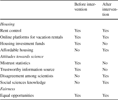
	Before intervention	After intervention
Housing
Rent control	Yes	Yes
Online platforms for vacation rentals	Yes	Yes
Housing investment funds	Yes	No
Affordable housing	No	Yes
Attitudes towards science
Mistrust statistics	Yes	No
Trustworthy information source	Yes	No
Disagreement among scientists	No	Yes
Social sciences knowledge	No	Yes
Fairness
Equal opportunities	Yes	Yes

Appendix 2: The video and the texts

Appendix 2.1: The refutational text

This the English translation of the original RT in Spanish. The text is 671 words long in Spanish, as shown in Table 11, and 599 words long in English. To clarify the refutational elements of the RT and to compare it with the NRT we number each paragraph as P1, P2, .... This enumeration was not included in the original text.

[P1] Prices of most products and services are the outcome of the interaction between many buyers on one hand and many sellers on the other hand. Sometimes governments, either national or local, regulate some prices.

[P2] For instance, public institutions set a price ceiling when buyers consider that the market price is too high. Or they set a price floor when sellers consider that the market price is too low.

[P3] Current economic research shows that when a price ceiling is set in a market, with the purpose of helping buyers, sooner or later this will lead to a drop in the quantity supplied by sellers.

[P4] In the case of rental housing, rents have increased substantially in recent years in many Spanish cities. Many families and young people struggle to pay these rents, yet, housing is a basic need. The difficulty many families and young people have in accessing decent housing is a serious social problem. The natural concern for this problem drives many people to think that the solution would be regulating rents through a price ceiling. However, plenty of research by social scientists debunk this belief.

[P5] Controlling rents is certainly an appealing proposal because it apparently could solve rental housing affordability in a very simple way. However, in reality, contrary to what it seems, this policy does not guarantee more access to housing precisely for people who are the most needy (low-income families and young adults). How can this be? Let’s think slowly and ask what has happened in cities where this policy has been carried out.

[P6] Many of the studies that investigate the effects of this policy in cities across the world conclude that it has brought about several important problems. For instance Swedish researchers Andersson and Söderberg in their study “Elimination of rent control in the Swedish rental housing market: Why and how?”, published in the academic journal Journal of Housing Research in 2012 (you can find it HERE) show that rent controls in Stockholm have led to long waiting lists, so that it takes about 10 years or more to find a house to rent (you can find it HERE). The bottom line is that, with rent regulation, many people search for a house to rent but very few dwellings are available.

[P7] This body of research also shows that this policy often brings about a black rental market. For instance, money is paid to advance a position in the queue, or dwellings are illegally sublet at prices above the legal ceiling.

[P8] Studies also show that under this policy some owners decide to sell their property instead of renting it; or decide to leave it empty because they consider that renting at the legal price ceiling is not worthwhile for them.

[P9] The conclusion of the research by social scientists is that with rent ceilings the supply of rental housing ends up falling, so that over time, the housing problem gets worse. The bottom line is that it is low-income families who often most harmed by a policy that intended just the opposite.

[P10] This does not mean that nothing can be done. On the contrary, research by social scientists proposes alternative policies to rent regulation. These policies would definitively benefit low-income families without the damaging effects mentioned above.

[P11] The main alternative policies are (1) development of public rental housing; (2) taxing unused land; and (3) directly support families whose income falls below a certain threshold. Policies (1) and (2) will increase the amount of rental housing, thus bringing rents down for everybody. And policy (3) aims at providing direct support only to those who need it.

Note: in the first “you can find it HERE” sentence in [P6] we place the link to Andersson and Söderberg (Reference Andersson and Söderberg2012): https://aresjournals.org/doi/abs/10.5555/jhor.21.2.xv120w45816v3344. In the second “you can find it HERE” sentence we place the link that leads to the Stockholm Housing Agency: https://bostad.stockholm.se/Como-funciona/

Appendix 2.2: The refutational video

This appendix shows the slideshow from the video. Each slide below includes the English translation and the reference to the RT paragraphs [P1], [P2], ...in Appendix B.1 where that sentence (or a similar one) can be found. The RV can be found at the following link: https://youtu.be/s5sr_vOrRMc. We use https://www.canva.com/ to develop the video.

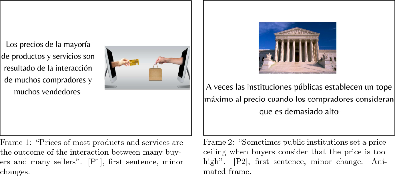
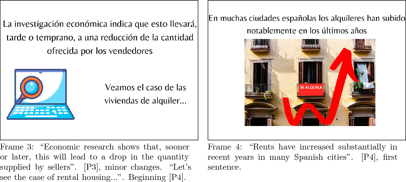
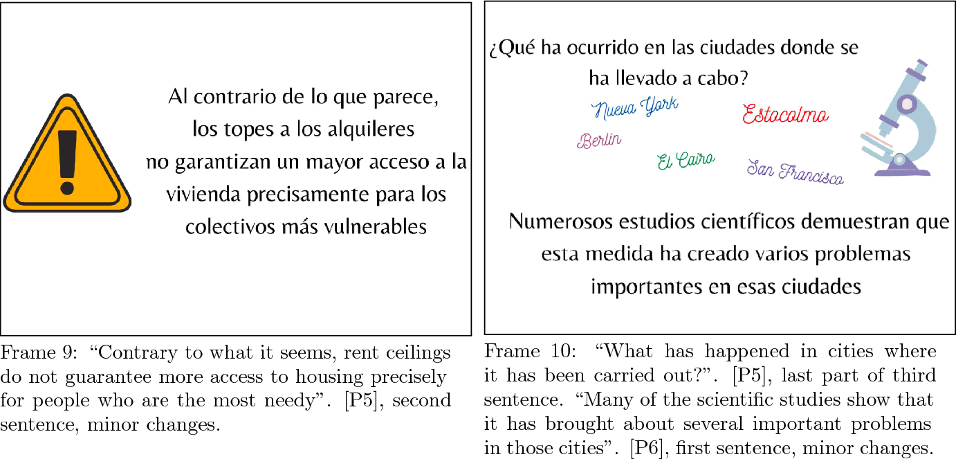
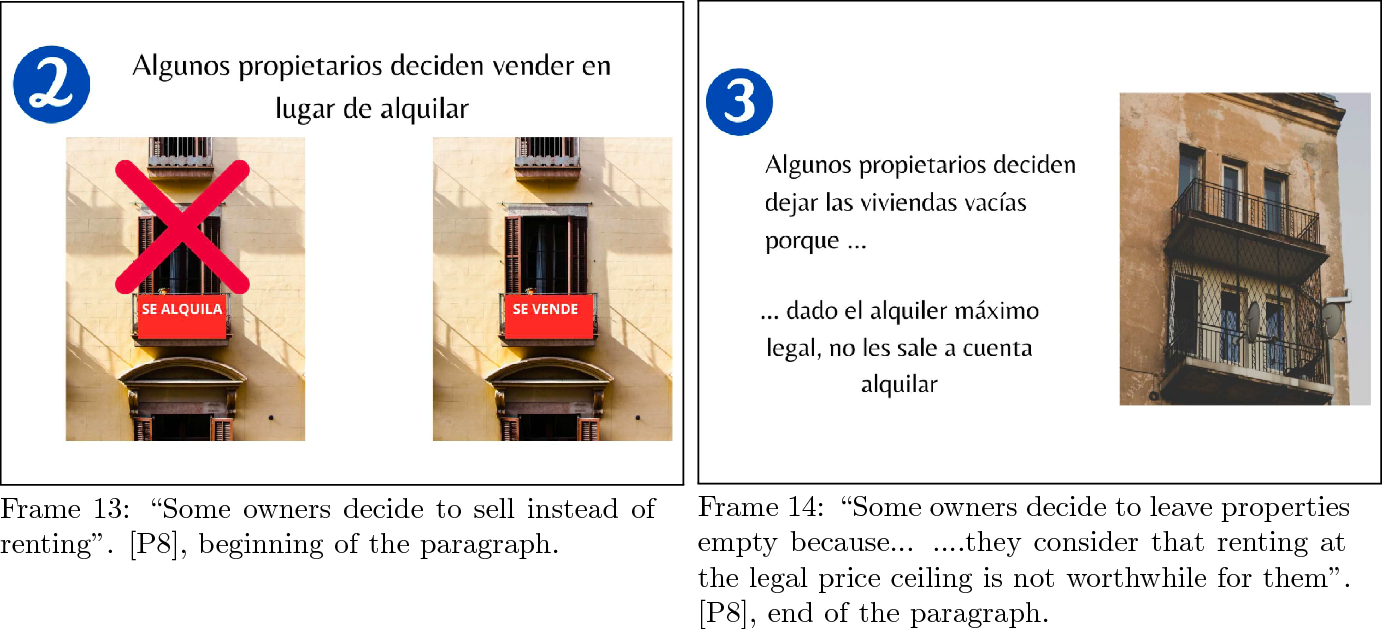
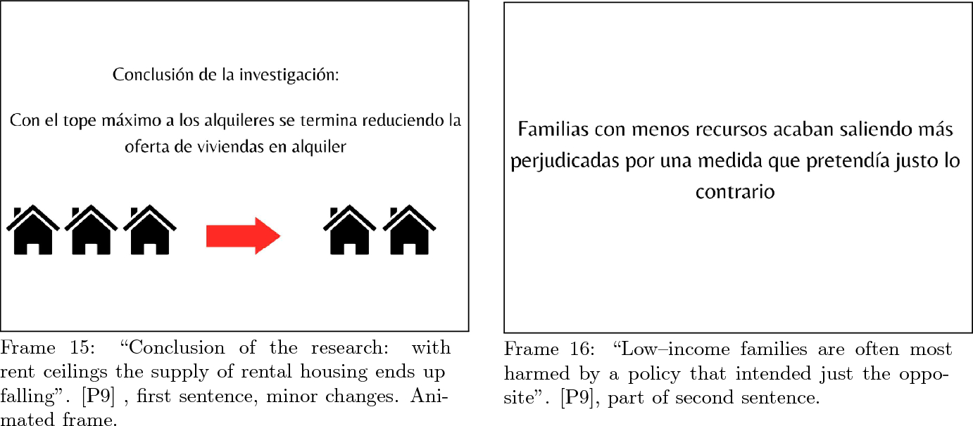
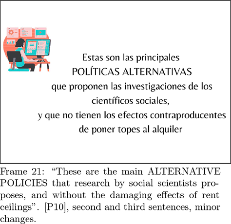
Appendix 2.3: The non-refutational (expository) text

This the English translation of the original NRT in Spanish. The text is 392 words long in Spanish, as shown in Table 11, and 349 words long in English. To compare the NRT with the RT we number each paragraph as P1, P2, .... This enumeration was not included in the original text.

[P2] For instance, public institutions set a price ceiling when buyers consider that the market price is too high. Or they set a price floor when sellers consider that the market price is too low.

[P3] Current economic research shows that when a price ceiling is set in a market, with the purpose of helping buyers, sooner or later this will lead to a drop in the quantity supplied by sellers.

[P4] Regarding the proposal of setting a rent ceiling, many of the studies that investigate the effects of this policy in cities across the world conclude that this is not the solution to facilitate access to housing. On the contrary, rent regulation can create bigger problems.

[P5] For instance Swedish researchers Andersson and Söderberg in their study “Elimination of rent control in the Swedish rental housing market: Why and how?”, published in the academic journal Journal of Housing Research in 2012 (you can find it HERE) show that rent controls in Stockholm have led to long waiting lists, so that it takes about 10 years or more to find a house to rent (you can find it HERE). The bottom line is that, with rent regulation, many people search for a house to rent but very few dwellings are available.

[P6] This body of research also shows that this policy often brings about a black rental market. For instance, money is paid to advance a position in the queue, or dwellings are illegally sublet at prices above the legal ceiling.

[P7] Studies also show that under this policy some owners decide to sell their property instead of renting it; or decide to leave it empty because they consider that renting at the legal price ceiling is not worthwhile for them.

[P8] The conclusion of the research by social scientists is that with rent ceilings the supply of rental housing ends up falling, so that over time, the housing problem gets worse.

Note: in the first “you can find it HERE” sentence in [P5] we place the link to Andersson and Söderberg (Reference Andersson and Söderberg2012): https://aresjournals.org/doi/abs/10.5555/jhor.21.2.xv120w45816v3344. In the second “you can find it HERE” sentence we place the link that leads to the Stockholm Housing Agency: https://bostad.stockholm.se/Como-funciona/

Appendix 2.4: Text readability and statistics

See Tables 10 and 11.

Table 10 Readability statistics (for the texts in Spanish)

Readability indexes	Non-refutational text		Refutational text
Readability indexes	Value	Easiness	Value	Easiness
Fernández Huerta	60.4	Standard (7th grade)	62.67	Standard (7th grade)
Gutiérrez de Polini (understandability)	38.78	Standard	39.57	Standard
Szigriszt–Pazos	55.72	Standard	58.21	Standard
INFLESZ–Barrio	55.72	Standard	58.21	Standard
Readability $μ$	52.5	Fairly difficult	50.57	Difficult

Fernandez Huerta index for Spanish is equivalent to the Flesch readability formula for English language. Szigriszt-Pazos index is an adaptation to Spanish language of the Flesch formula for English. INFLESZ Barrio index adapts the Szigriszt-Pazos index to the current average Spanish reader. Readability statistics are obtained from this website: https://legible.es/

Table 11 Text statistics (for the texts in Spanish)

	Non-refutational text	Refutational text
Estimated read time	2 minutes	3.4 minutes
No. of characters	2420	4268
No. of letters	1971	3484
No. of syllables	821	1447
No. of words	392	671
No. of sentences	18	46
No. of paragraphs	8	11
Average letters per word	5.03	5.19
Average syllables per word	2.09	2.16
Average words per sentence	20.63	14.28

Text statistics obtained from this website: https://legible.es/

Appendix 2.5: Comprehension questions

• Question 1 (correct answer is C):

The text/video exposes that:
1. A. Rents in Spain have increased up to the price ceiling.
2. B. If the Government or the City council establishes a rent capping, many people will have easier access to housing.
3. C. Establishing a rent capping may create problems and not achieve its objective of facilitating access to housing.
• Question 2 (correct answer is B):

The text/video suggests that:
1. A. Rental vacation apartments have mostly contributed to the increase in rents in certain areas.
2. B. Regulating rents through a price ceiling may lead to different forms of corruption.
3. C. Setting a rent capping will guarantee that all low-income people may access to housing.

Appendix 3: Additional results

See Tables 12, 13 , 14 and 15.

Table 12 Characteristics of participants in each condition

	NRT	RT	RV	Difference	Difference	Difference
				(NRT–RT)	(RT–RV)	(NRT–RV)
Female	0.50	0.50	0.48	0.00	0.02	0.02
Non-Spanish	0.06	0.05	0.08	0.01	$-$ 0.03	$-$ 0.01
Age	30.19	33.22	30.99	$-$ 3.03***	2.22**	$-$ 0.80
(st. dev.)	(12.76)	(14.28)	(11.51)
Education level:
Primary or less	0.03	0.07	0.01	$-$ 0.04**	0.05***	0.02*
Compulsory	0.09	0.11	0.12	$-$ 0.01	$-$ 0.01	$-$ 0.02
Upper secondary	0.44	0.38	0.37	0.06*	0.01	0.07*
Tertiary	0.44	0.45	0.50	$-$ 0.01	$-$ 0.05	$-$ 0.06
Currently enrolled in TEd.	0.51	0.39	0.41	0.12***	$-$ 0.02	0.10***
Labor status:
Employed	0.38	0.46	0.50	$-$ 0.08**	$-$ 0.04	$-$ 0.12***
Unemployed	0.13	0.13	0.12	0.01	0.00	0.01
Not in labor force	0.46	0.37	0.35	0.09**	0.02	0.11***
Furlough	0.03	0.04	0.01	$-$ 0.02	0.04***	0.02**
Province:
Alicante	0.07	0.05	0.06	0.02	$-$ 0.01	0.01
Barcelona	0.03	0.05	0.06	$-$ 0.02	$-$ 0.01	$-$ 0.02
Madrid	0.08	0.09	0.16	$-$ 0.01	$-$ 0.06**	$-$ 0.08***
Valencia	0.59	0.50	0.42	0.09**	0.08**	0.17***
Other	0.23	0.30	0.31	$-$ 0.07**	$-$ 0.00	$-$ 0.08**
Home ownership:
Owner	0.38	0.40	0.38	$-$ 0.02	0.01	$-$ 0.00
Mortgage	0.30	0.33	0.26	$-$ 0.02	0.07**	0.05
Tenant	0.20	0.19	0.18	0.01	0.01	0.02
Other	0.12	0.09	0.18	0.03	$-$ 0.09***	$-$ 0.06**
Household composition:
Single	0.11	0.13	0.14	$-$ 0.01	$-$ 0.01	$-$ 0.02
Single parent	0.21	0.22	0.17	$-$ 0.01	0.05	0.04
Childless couple	0.10	0.09	0.13	0.01	$-$ 0.04*	$-$ 0.03
Couple with children	0.45	0.48	0.37	$-$ 0.03	0.11***	0.08**
Other	0.13	0.09	0.19	0.04	$-$ 0.10***	$-$ 0.07**
Town size:
Small	0.13	0.13	0.14	0.00	$-$ 0.01	$-$ 0.00
Medium	0.42	0.47	0.40	$-$ 0.05	0.07*	0.02
Large	0.45	0.40	0.47	0.04	$-$ 0.06*	-0.02
Observations	351	351	362

RV Refutational video. RT Refutational text. NRT Non-refutational text. TEd. Tertiary education. Significance levels of t-tests of the difference in means: * $p < 0.10$ , ** $p < 0.05$ , *** $p < 0.01$

Table 13 Statistics of time spent in each screen in minutes

	Mean	Std. Dev.	Min.	Max.
A. Non-refutation text condition (N $=$ 351)
All screens	13.51	8.17	1.13	44.78
Instructions screen	0.72	1.55	0.02	23.83
Sociodemographic quest. screen	1.67	1.54	0.27	17.47
Initial opinion quest. screen	1.67	1.61	0.15	16.57
Text screen	2.12	1.96	0.03	20.93
Comprehension questions screen	1.01	1.62	0.05	22.32
CRT screen	5.20	4.50	0.28	34.77
Final opinion quest. screen	1.14	1.49	0.10	25.33
Closing screen	0.14	0.17	0.02	1.97
B. Refutation text condition (N $=$ 351)
All screens	12.76	9.16	1.05	60.03
Instructions screen	0.61	1.25	0.02	14.90
Sociodemographic quest. screen	1.47	1.16	0.25	8.70
Initial opinion quest. screen	1.45	1.54	0.10	14.10
Text screen	2.80	2.74	0.02	18.08
Comprehension questions screen	0.93	1.38	0.05	14.80
CRT screen	4.40	4.17	0.18	27.83
Final opinion quest. screen	1.09	1.26	0.08	16.25
Closing screen	0.17	0.37	0.00	5.30
C. Refutation video condition (N $=$ 362)
All screens	13.40	8.08	1.12	55.87
Instructions screen	0.69	1.45	0.02	21.73
Sociodemographic quest. screen	1.50	1.51	0.25	18.72
Initial opinion quest. screen	1.33	0.94	0.12	5.50
Video screen	3.26	2.44	0.02	14.95
Comprehension questions screen	0.72	0.84	0.05	8.93
CRT screen	4.82	4.02	0.20	23.72
Final opinion quest. screen	1.08	1.19	0.12	15.75
Closing screen	0.17	0.28	0.02	3.35

CRT Cognitive Reflection Test

Table 14 Estimated treatment effects on revising the misconception

	RV vs. RT		RT vs. NRT		RV vs. NRT		Pooled $^{†}$
	(1)	(2)	(3)	(4)	(5)	(6)	(7)	(8)
RV	0.17	0.18*	–	–	0.23**	0.26***	0.17	0.19*
RV	(0.10)	(0.11)			(0.10)	(0.10)	(0.10)	(0.10)
RT	–	–	0.06	0.07	–	–	–	–
RT			(0.10)	(0.10)
NRT	–	–	–	–	–	–	$-$ 0.06	$-$ 0.07
NRT							(0.10)	(0.10)
Female		0.26**		0.12		0.08		0.16*
Female		(0.11)		(0.10)		(0.10)		(0.08)
Non-Spanish		0.27		0.13		0.21		0.22
Non-Spanish		(0.22)		(0.22)		(0.19)		(0.17)
Age		$-$ 0.01***		$-$ 0.01**		$-$ 0.02***		$-$ 0.01***
Age		(0.01)		(0.01)		(0.01)		(0.00)
Education level:
Compulsory		$-$ 1.02***		$-$ 0.29		$-$ 0.40		$-$ 0.63**
Compulsory		(0.31)		(0.26)		(0.39)		(0.25)
Upper secondary		$-$ 0.82***		$-$ 0.45*		$-$ 0.55		$-$ 0.66***
Upper secondary		(0.29)		(0.25)		(0.38)		(0.24)
Tertiary		$-$ 0.77***		$-$ 0.35		$-$ 0.40		$-$ 0.57**
Tertiary		(0.28)		(0.24)		(0.38)		(0.23)
Enrolled in TEd.		0.08		$-$ 0.18		0.22		0.05
Enrolled in TEd.		(0.16)		(0.14)		(0.15)		(0.12)
Labor status:
Unemployed		0.03		0.03		$-$ 0.13		$-$ 0.04
Unemployed		(0.17)		(0.16)		(0.16)		(0.13)
Not in labor force		$-$ 0.09		$-$ 0.15		$-$ 0.19		$-$ 0.15
Not in labor force		(0.14)		(0.13)		(0.14)		(0.11)
Furlough		$-$ 0.51		$-$ 0.12		0.35		$-$ 0.15
Furlough		(0.35)		(0.27)		(0.31)		(0.27)
Province:
Barcelona		0.86***		0.08		0.82***		0.56**
Barcelona		(0.30)		(0.30)		(0.28)		(0.24)
Madrid		0.11		$-$ 0.73***		0.08		$-$ 0.18
Madrid		(0.27)		(0.27)		(0.25)		(0.22)
Valencia		0.44**		$-$ 0.23		0.24		0.13
Valencia		(0.22)		(0.22)		(0.20)		(0.17)
Other		0.35		$-$ 0.45**		0.18		0.01
Other		(0.22)		(0.22)		(0.21)		(0.18)
Home ownership:
Mortgage		$-$ 0.05		$-$ 0.13		0.07		$-$ 0.03
Mortgage		(0.13)		(0.12)		(0.12)		(0.10)
Tenant		$-$ 0.18		$-$ 0.21		$-$ 0.08		$-$ 0.16
Tenant		(0.17)		(0.15)		(0.17)		(0.13)
Other		$-$ 0.12		$-$ 0.21		0.03		$-$ 0.07
Other		(0.20)		(0.19)		(0.20)		(0.16)
Household composition:
Single parent		0.23		0.04		0.09		0.11
Single parent		(0.18)		(0.17)		(0.19)		(0.15)
Childless couple		0.54**		0.25		0.17		0.32*
Childless couple		(0.21)		(0.20)		(0.21)		(0.17)
Couple with children		0.36**		0.42***		0.25		0.34***
Couple with children		(0.16)		(0.15)		(0.16)		(0.13)
Other		0.21		0.42**		0.05		0.20
Other		(0.21)		(0.20)		(0.21)		(0.17)
Town size:
Medium		$-$ 0.08		$-$ 0.09		0.07		$-$ 0.02
Medium		(0.16)		(0.16)		(0.16)		(0.13)
Large		0.03		$-$ 0.02		$-$ 0.02		0.00
Large		(0.17)		(0.16)		(0.16)		(0.13)
Constant	1.00***	1.53***	0.94***	1.93***	0.94***	1.38***	1.00***	1.71***
Constant	(0.07)	(0.47)	(0.06)	(0.45)	(0.06)	(0.51)	(0.07)	(0.38)
Observations	713	713	702	702	713	713	1064	1064
$R^{2}$	0.00	0.07	0.00	0.06	0.01	0.05	0.01	0.05

Dependent variable: belief change after intervention; it takes values between $- 4$ and 4 (positive values indicate a change away from the misconception). RT: Refutational text. NRT: Non-refutational text. RV: Refutational video. Pooled†: pooled sample with all three conditions. TEd.: Tertiary education. Robust standard errors in parentheses. Reference categories: primary education, employed, Alicante, owner, single, small size. Significance levels: *p<0.10, **p<0.05, ***p<0.01

Table 15 Correlation of initial belief with CRT and socio-demographic variables

	RV	RT	NRT
CRT	0.08	$-$ 0.06	$-$ 0.04
CRT	(0.23)	(0.24)	(0.24)
Female	$-$ 0.34***	$-$ 0.27**	$-$ 0.10
Female	(0.11)	(0.11)	(0.11)
Non-Spanish	0.38	$-$ 0.02	0.03
Non-Spanish	(0.24)	(0.26)	(0.23)
Age	0.02**	0.00	0.02***
Age	(0.01)	(0.01)	(0.01)
Education level:
Compulsory	0.62	0.20	$-$ 0.16
Compulsory	(0.73)	(0.25)	(0.42)
Upper secondary	0.59	0.42*	0.11
Upper secondary	(0.73)	(0.22)	(0.41)
Tertiary	0.58	0.28	0.14
Tertiary	(0.73)	(0.23)	(0.42)
Enrolled in TEd.	0.04	0.02	0.28*
Enrolled in TEd.	(0.18)	(0.19)	(0.16)
Labor status:
Unemployed	$-$ 0.00	$-$ 0.20	$-$ 0.22
Unemployed	(0.19)	(0.18)	(0.21)
Not in labor force	0.14	0.08	$-$ 0.04
Not in labor force	(0.17)	(0.18)	(0.15)
Furlough	$-$ 0.14	0.67**	0.06
Furlough	(1.01)	(0.27)	(0.33)
Province:
Barcelona	$-$ 0.46	$-$ 0.81**	$-$ 0.79**
Barcelona	(0.30)	(0.33)	(0.34)
Madrid	$-$ 0.06	$-$ 0.38	0.37
Madrid	(0.27)	(0.37)	(0.33)
Valencia	$-$ 0.08	$-$ 0.28	0.02
Valencia	(0.24)	(0.30)	(0.25)
Other	$-$ 0.12	$-$ 0.42	0.21
Other	(0.25)	(0.31)	(0.28)
Home ownership:
Mortgage	0.08	0.20	0.18
Mortgage	(0.15)	(0.14)	(0.14)
Tenant	$-$ 0.21	0.30	0.09
Tenant	(0.17)	(0.18)	(0.17)
Other	0.26	0.33	0.35
Other	(0.23)	(0.23)	(0.21)
Household composition:
Single parent	$-$ 0.06	$-$ 0.14	0.17
Single parent	(0.21)	(0.22)	(0.21)
Childless couple	$-$ 0.16	$-$ 0.43*	$-$ 0.22
Childless couple	(0.21)	(0.25)	(0.24)
Couple with children	0.09	$-$ 0.25	$-$ 0.12
Couple with children	(0.18)	(0.19)	(0.19)
Other	0.00	$-$ 0.31	$-$ 0.17
Other	(0.22)	(0.28)	(0.24)
Town size:
Medium	0.20	$-$ 0.03	0.20
Medium	(0.18)	(0.21)	(0.19)
Large	0.19	$-$ 0.17	$-$ 0.02
Large	(0.19)	(0.21)	(0.18)
Constant	1.01	2.30***	1.02
Constant	(0.91)	(0.51)	(0.67)
N	362	351	351
$R^{2}$	0.08	0.10	0.13

Dependent variable takes values from 5 (fully disagree) to 1 (fully agree). RV Refutational video. RT Refutational text. NRT Non-refutational text. TEd. Tertiary education. Robust standard errors in parentheses. Significance levels: * $p < 0.10$ , ** $p < 0.05$ , *** $p < 0.01$

Appendix 4: Cognitive reflection test

The test contains adapted versions of the three initial Frederick (Reference Frederick2005) (F) statements, of four statements taken from Thomson and Oppenheimer (Reference Thomson and Oppenheimer2016) (TO), and of one from Toplak et al. (Reference Toplak, West and Stanovich2014) (T).

1. A bat and a ball cost £1.10 in total. The bat costs a dollar more than the ball. How much does the ball cost? (F)

Adapted version: A bat and a ball cost €1.10 in total. The bat costs €1.00 more than the ball. How much does the ball cost?

2. If it takes 5 machines 5 minutes to make 5 widgets, how long would it take 100 machines to make 100 widgets? (F)

3. In a lake, there is a patch of lily pads. Every day, the patch doubles in size. If it takes 48 days for the patch to cover the entire lake, how long would it take for the patch to cover half the lake? (F)

Adapted version: In Europe the demand for electric kick scooters is expanding. Every month, demand doubles. If it takes 48 months for demand to reach its full potential, how many months will it take for demand to reach one half of its potential?

4. If you’re running a race and you pass the person in second place, what place are you in? (TO)

Adapted version: Your business appears in a sales ranking chart. If next year your business surpasses the business in second place, what place will you be in?

5. A farmer had 15 sheep and all but 8 died. How many are left? (TO)

Adapted version: A fruit store has bought 15 tomato boxes, and all but 8 have been damaged. How many are left?

6. Emily’s father had three daughters. The first two are named April and May. What is the third daughter’s name? (TO)

Adapted version: The family, who owns the firm FOC, which produces firecrackers and pyrotechnic products, owns a total of three firms. The first two are named PIM and PAM. How is the third named?

Note: PIM, PAM, PUM is a popular onomatopoeic expression in Spanish that represents shots or explosions. It also refers to a game in which you try to knock down balls in a row.

7. How many cubic feet of dirt are there in a hole that is 3’ deep x 3’ wide x 3’ long? (TO)

Adapted version: A developer buys a plot to build a public sport center. In the plot there is a hole measuring 3 meters deep x 3 meters wide x 3 meters long. How many cubic meters of dirt are there in the hole?

8. A man buys a pig for €60, sells it for €70, buys it back for €80, and sells it finally for €90. How much has he made? (T)

Adapted version: Someone buys a videogame for €60, sells it for €70, buys it back for €80, and sells it finally for €90. How much has this person made?

Appendix 5: Instructions to participants

Instructions are the same across conditions.

Appendix 5.1: Initial instructions

You are about to participate in an activity to gather opinions about economic and social issues.

To complete the different tasks that you will face you will receive an economic compensation of 6 EUROS. This amount will be paid to you through PayPal. The tasks should take you about 20 minutes, but you can take more time if you wish. You have a total of one hour to complete everything.

One of the activities we will ask you to do will allow you to EARN 2 EXTRA EUROS in case you do it correctly. Hence, if you do this task activity correctly you will receive an economic compensation of in TOTAL $6 + 2 = 8$ EUROS. We will inform you about whether you have obtained the 2 extra euros after you will have completed all the tasks that we will ask you to do.

In this activity that you are about to begin we will ask you, first, to provide us with some socio-demographic information.

Subsequently, we will ask you opinion about some economic and social issues. There is no correct or incorrect answer for these questions. We just ask you about your sincere opinion, and your answers will not influence your final payment.

Then we will present to a short text (video). We will appreciate that you read it (watch it) carefully and then answer two questions directed a checking the comprehension of the text (the video). If you respond correctly to the two questions you will receive 2 euros extra in your final payment.

Subsequently, we will present some economic situations to you. Your responses to these situations will not influence your final payment.

Finally, we will ask you opinion about some economic and social issues. There is no correct or incorrect answer for these questions. We just ask you about your sincere opinion, and your answers will not influence your final payment.

All your responses will be anonymized.

This activity is part of social research project carried out by professors from several universities. Your effort and attention in answering all questions will be very valuable for the success of this study, contributing to a better understanding of our society.

We thank you in advance for your collaboration!

Appendix 5.2: Other instructions

- Before opinion questionnaires:

We next will show you several statements about economic and social issues. Please read them carefully and choose the option that best matches your current opinion. There is no correct or incorrect answer for these questions. We just wish to know your sincere opinion, and your answers will NOT AFFECT your final payment.

- Before the video:

We next will show you a video. Please watch it carefully. You may pause it and replay it if you wish. You will next be presented with two questions. These questions refer to the video, but to answer them you will not be able to view the video again. If your answers to both questions are correct, you will additionally win 2 euros at the end. You therefore will have the chance to win a total of 8 euros.

Press PLAY to start the video.

- Before the texts:

Next we will show you a text. We ask you to read it carefully and then answer 2 questions that will appear in the next screen. These questions relate to the text you will just have read, but you will not be able to read the text again to answer them. If your answers to both questions are correct, you will additionally win 2 euros at the end. You therefore will have the chance to win a total of 8 euros.

- Before the comprehension questions:

Next you will see 2 questions about the text [video] you just have read [watched]. Please indicate, for each question, which of the statements you think is correct. If your answers to both questions are correct, you will additionally win 2 euros at the end. You therefore will have the chance to win 8 euros in total. After the questions, we will tell you how many are correct as well as the amount you have won.

- Before CRT:

We next will show you some economic situations. Please read them carefully and answer the questions. Your answers DO NOT AFFECT your final payment.

- Before the final opinion questionnaire:

You will see next some statements about economic and social issues. Please read them carefully and choose the option closer to your personal opinion at this moment. There are no correct or incorrect answers. We only wish to know your sincere opinion, and your answers WILL NOT AFFECT the final payment.

Footnotes

We thank the editor, a co-editor and two anonymous referees for their constructive comments. We also acknowledge financial support from the Call for Experimental Research Projects in the Social Sciences from The Social Observatory of “la Caixa” Foundation and financial support from the Spanish Ministry of Science and Innovation PID2020-112739GA-I00 (Lopez-Mayan), PID2020-114251GB-I00 (Brandts and Lopez-Mayan), PID2021-122605NB-I00 funded by MCIN7AEI/10.13039/501100011033 and ERDF A way of making Europe, and Generalitat de Catalunya, grant 2021 SGR 00571 (Panadés), PID2021-124713OB-I00 (Busom) and the Spanish Agencia Estatal de Investigación (AEI), through the Severo Ochoa Programme for Centres of Excellence in R &D (Barcelona School of Economics CEX2019-000915-S) (Brandts and Panadés). This work complies with the ethical requirements of Universitat de Valencia. We are also grateful for the comments from participants at the 2022 Lisbon Economics and Statistics of Education Conference, the 12th International Workshop on Applied Economics of Education in Catanzaro, the 14th Maastricht Behavioral and Experimental Economics Symposium, the 12th International Conference of the French Association of Experimental Economics (ASFEE), 47th Symposium of the Spanish Economic Association (SAEe), the 2023 Royal Economic Society Annual Conference, the 3rd Catalan Economic Society Conference, the 7th International Meeting on Experimental and Behavioral Social Sciences (IMEBESS), the CESifo Venice Summer Institute 2023—People’s understanding and support for economic policies, the 2023 Economic Science Association World Meeting, and seminar presentations at the WU in Vienna and Loyola University Andalucía. Anonymized copies of the preregistered plans are available at https://aspredicted.org/blind.php?x=uv2t69 and https://aspredicted.org/blind.php?x=4n78sy. This paper was previously circulated under the title “Pictures are worth many words: Effectiveness of visual communication in dispelling the rent-control misconception”. The replication material for the study is available at https://doi.org/10.34810/data897.

¹ In Spain, a poll conducted in 2023 by 40dB on behalf of the media Cadena Ser/El País found that 75% of respondents support rent control. In Germany, 71% of respondents to a poll conducted by Infratest dimap in 2020 were in favor of the rent cap in Berlin. In the UK, the support for rent controls reached 71% in a poll conducted in December 2019 by Ipsos MORI, with only 9% of people opposing them. This is the most supported policy among other housing policies indicated in the same survey. Building new public homes is supported by 56%, while opposed by 15%. In a poll conducted by the Institute of Governmental Studies (IGS) of UC Berkeley in 2017, 60% of the state’s registered voters favored rent control, while 26% opposed them.

² Percentage weighted by the degree of confidence of the response. See https://www.igmchicago.org/surveys/rent-control/

³ See also Stockholm’s housing agency, https://bostad.stockholm.se/english/.

⁴ The on-line experiment was preregistered at AsPredicted Registry, Wharton Credibility Lab, University of Pennsylvania.

⁵ There is no consensus on the terminology that refers to attributes other than cognitive ability. Here we adopt the term personality traits. Other authors refer to them as non-cognitive abilities, character skills, temperament or personal qualities. All this terminology has flaws as discussed in Duckworth and Yeager (Reference Duckworth and Yeager2015).

⁶ Given our limited budget, we could not test the effectiveness of another possible visual treatment, a non-refutational video. Our previous work in Brandts et al. (Reference Brandts, Busom, Lopez-Mayan and Panadés2022) shows some indication that the refutational text correction improves slightly relative to the expository text. We decided here to keep the refutational approach, now combining it with visual elements, to test whether the effectiveness of this format of communication is stronger than the RT format.

⁷ An anonymized copy, without author names, of the first preregistered plan is available at https://aspredicted.org/blind.php?x=uv2t69. The PAP corresponding to the video condition is available at https://aspredicted.org/blind.php?x=4n78sy.

⁸ A fifth element refers to facilitating interactions among individuals by asking them to explain their opinions to other participants. We do not introduce this element here because of the technical complexity involved in an online setting.

⁹ First link: https://aresjournals.org/doi/abs/10.5555/jhor.21.2.xv120w45816v3344. Second link: https://bostad.stockholm.se/Como-funciona/ Both links are also included in the NRT below

¹⁰ Due to technical complexity, it was not possible to include in the RV the two links inserted in the RT.

¹¹ We thank a professional in the visual industry for his advice about the suitability of the sequences of images and signs.

¹² When the misconception on rent controls is not explicitly addressed, undergraduate students are found to stick to it after receiving standard teaching on price controls during a course in principles of economics, even if they perform well in a question on this topic included in graded tests (Busom et al., Reference Busom, Lopez-Mayan and Panadés2017).

¹³ To see how our sample compares to the adult population in Spain, we use the information from the March 2023 Barometer sample from the Spanish Centro de Investigaciones Sociologicas, CIS (Sociological Research Center). CIS is the national public entity in charge of regularly conducting opinion surveys on a range of socio-economic and political topics. Its sample includes individuals 18 years old or older, as is our case. In this sample, 52% of people are women, 20% younger than 34 years of age, 4% non-Spanish. The distribution of education levels is: primary or less 8.4%, compulsory 13%, upper secondary 34%, tertiary 44%. The employed are 54%, the unemployed 9%, not in labor force 36%. With respect to housing, 47% are owners, 29% have a mortgage, 19% are tenants, and other 5.4%. CIS does not provide data on household composition, municipality size and province of residence. We thus use information from the Spanish Statistics Institute (INE). According to the 2020 Household Survey, household composition is: single 26%, single parent 10.4%, childless couple 21%, couple with children 33%. According to the 2021 Census, the distribution of the population by town size is 20% small, 40% medium and 40% large; the share of population living in Valencia is around 6%. Therefore, our samples for each treatment are quite representative for gender, non-Spanish, education, labor status, home ownership, and less so for household composition and town size. For age distribution and province of residence the differences are large. We should clarify that our limited budget did not allow for a complete stratification of the sample to obtain a fully representative sample of the adult Spanish population. Nevertheless, the level of representativeness of our sample is quite high in many important dimensions.

¹⁴ Note that rents are unregulated in Spain since the 1980s; only in May 2023 the Spanish Parliament passed a law that allows regional governments to set rent control regulations. At the local level, however, only the municipality of Barcelona and some other municipalities in Catalonia with tight housing markets were subject to rent control during the period September 2020 to April 2022. About 3 to 6% of our participants live in the province of Barcelona, depending on the condition. Not all municipalities were regulated, and although we do not have information about the participants’ municipality of residence, we can conclude that very few participants potentially live in a regulated area. Therefore, it is very unlikely that this factor drives the results.

¹⁵ A potential concern in experimental work is the presence of an experimenter demand effect. Note that all three interventions would be equally subject to this effect, and what we do is to compare across conditions.

¹⁶ We add up agree and totally agree; and disagree and totally disagree.

¹⁷ The pooled estimation conditional on initial beliefs yields the same results.

Springer Nature remains neutral with regard to jurisdictional claims in published maps and institutional affiliations.

References

Aguilar, S. J., Polikoff, M. S., & Sinatra, G. M. (2019). Refutation texts: A new approach to changing public misconceptions about education policy. Educational Researcher, 48(5), 263–272. 10.3102/0013189X19849416CrossRef Google Scholar

Ahern, K. R., & Giacoletti, M. (2022). ‘Robbing Peter to pay Paul? The redistribution of wealth caused by rent control. NBER Working Paper 30083.CrossRef Google Scholar

Alesina, A., Ferroni, M. F., & Stantcheva, S. (2021). Perceptions of racial gaps, their causes, and ways to reduce them. NBER Working Paper 29245.CrossRef Google Scholar

Andersson, R., & Söderberg, B. (2012). Elimination of rent control in the Swedish rental housing market: Why and how?. Journal of Housing Research, 21(2), 159–181. 10.1080/10835547.2012.12092062CrossRef Google Scholar

Asquith, B. J. (2019). Do rent increases reduce the housing supply under rent control? Evidence from evictions in San Francisco. Upjohn Institute Working Paper 19–296.CrossRef Google Scholar

Barrera, O., Guriev, S., Henry, E., & Zhuravskaya, E. (2020). Facts, alternative facts, and fact checking in times of post-truth politics. Journal of Public Economics, 182. 10.1016/j.jpubeco.2019.104123CrossRef Google Scholar

Bó, E. D., Bó, P. D., & Eyster, E. (2018). The demand for bad policy when voters underappreciate equilibrium effects. The Review of Economic Studies, 85, 964–998. 10.1093/restud/rdx031Google Scholar

Bolsen, T., Palm, R., & Kingsland, J. (2019). Counteracting climate science politicization with effective frames and imagery. Science Communication, 41(2), 147–171. 10.1177/1075547019834565CrossRef Google Scholar

Brandts, J., Busom, I., Lopez-Mayan, C., & Panadés, J. (2022). Dispelling misconceptions about economics. Journal of Economic Psychology, 88. 10.1016/j.joep.2021.102461CrossRef Google Scholar

Busom, I., Lopez-Mayan, C., & Panadés, J. (2017). Students’ persistent preconceptions and learning economic principles. The Journal of Economic Education, 48(2), 74–92. 10.1080/00220485.2017.1285735CrossRef Google Scholar

Chan, M. S., Jones, C. R., Jamieson, K. H., & Albarracín, D. (2017). Debunking: A meta-analysis of the psychological efficacy of messages countering misinformation. Psychological Science, 28(11), 1531–1546. 10.1177/0956797617714579CrossRef Google Scholar PubMed

Coibion, O., Gorodnichenko, Y., & Weber, M. (2019). Monetary policy communications and their effects on household inflation expectations. NBER Working Paper 25482.CrossRef Google Scholar

Coibion, O., Gorodnichenko, Y., & Weber, M. (2020). ‘Does policy communication during covid work? NBER Working Paper 27384.CrossRef Google Scholar

Diamond, R., McQuade, T., & Qian, F. (2019). The effects of rent control expansion on tenants, landlords, and inequality: Evidence from San Francisco. American Economic Review, 109(9), 3365–3394. 10.1257/aer.20181289CrossRef Google Scholar

Diamond, R., McQuade, T., & Qian, F. (2019b). Who pays for rent control?. Heterogeneous landlord response to San Francisco’s rent control expansion’, AEA Papers and Proceedings, 109, 377–380.Google Scholar

Dolls, M., Schüle, P., & Windsteiger, L. (2022). Affecting public support for economic policies: Evidence from a survey experiment about rent control in Germany. CESifo Working Paper No. 10493.Google Scholar

Druckman, J. (2015). Communicating policy-relevant science. PS, Political Science & Politics, 48, 58–69. 10.1017/S1049096515000438CrossRef Google Scholar

Duckworth, A. L., & Yeager, D. S. (2015). Measurement matters: Assessing personal qualities other than cognitive ability for educational purposes. Educational Researcher, 44(4), 237–251. 10.3102/0013189X15584327CrossRef Google Scholar PubMed

Ecker, U. K., Lewandowsky, S., Cook, J., Schmid, P., Fazio, L. K., Brashier, N., Kendeou, P., Vraga, E. K., & Amazeen, M. A. (2022). The psychological drivers of misinformation belief and its resistance to correction. Nature Reviews Psychology, 1, 13–26. 10.1038/s44159-021-00006-yCrossRef Google Scholar

Ecker, U. K., O’Reilly, Z., Reid, J., & Chang, E. (2020). The effectiveness of short format refutational fact-checks. British Journal of Psychology, 111, 36–54. 10.1111/bjop.12383CrossRef Google Scholar PubMed

Elias, J., Lacetera, N., & Macis, M. (2022). Is the price right? The role of economic tradeoffs in explaining reactions to price surges. NBER WP, W29963(112), 163–169.Google Scholar

Ferrero, M., Konstantinidis, E., & Vadillo, M. A. (2020). An attempt to correct erroneous ideas among teacher education students: The effectiveness of refutation texts. Frontiers in Psychology, 11. 10.3389/fpsyg.2020.577738CrossRef Google Scholar PubMed

Frederick, S. (2005). Cognitive reflection and decision making. Journal of Economic Perspectives, 19(4), 25–42. 10.1257/089533005775196732CrossRef Google Scholar

Goldberg, M. H., van der Linden, S., Ballew, M. T., Rosenthal, S. A., Gustafson, A., & Leiserowitz, A. (2019). The experience of consensus: Video as an effective medium to communicate scientific agreement on climate change. Science Communication, 41(5), 659–673. 10.1177/1075547019874361CrossRef Google Scholar

Haaland, I., Roth, C., & Wohlfart, J. (2023). Designing information provision experiments. Journal of Economic Literature, 10.1257/jel.20211658CrossRef Google Scholar

Hahn, A. M., Kholodilin, K. A., & Waltl, S. R. (2021). Forward to the past: Short-term effects of the rent freeze in Berlin. DIW Discussion Paper No. 1928.Google Scholar

Haldane, A., & McMahon, M. (2018). Central bank communications and the general public. AEA Papers and Proceedings, 108, 578–583. 10.1257/pandp.20181082CrossRef Google Scholar

Henry, E., Zhuravskaya, E., & Guriev, S. (2021). Checking and sharing alt-facts. CEPR Discussion Paper 14738.Google Scholar

Hüning, H., Mechtenberg, L., & Wang, S. W. (2021). Changing opinions and votes with peer-to-peer communication: Experimental evidence from a rent control ballot measure. Downloaded from https://sites.pitt.edu/~swwang/papers/Rent_Control.pdf.Google Scholar

Kattenberg, M. A. C., & Hassink, W. H. J. (2017). Who moves out of social housing? The effect of rent control on housing tenure choice. De Economist 165(43–66).CrossRef Google Scholar

Kholodilin, K. A., & Kohl, S. (2020). Does social policy through rent controls inhibit new construction DIW Berlin Discussion Paper: Some answers from long-run historical evidence.CrossRef Google Scholar

Kowalski, P., & Taylor, A. K. (2009). The effect of refuting misconceptions in the introductory psychology class. Teaching of Psychology, 36, 153–159. 10.1080/00986280902959986CrossRef Google Scholar

Kowalski, P., & Taylor, A. K. (2017). Reducing students’ misconceptions with refutational teaching: For long-term retention, comprehension matters. Scholarship of Teaching and Learning in Psychology, 3(2), 90–100. 10.1037/stl0000082CrossRef Google Scholar

Krugman, P., & Wells, R. (2020). Essentials of Economics (5th ed.). Worth Publishers.Google Scholar

Lewandowsky, S. (2021). Climate change, disinformation, and how to combat it. Annual Review of Public Health,42,. https://doi.org/10.1146/annurev-publhealth-090419-102409.CrossRef Google Scholar

Lewandowsky, S., Ecker, U., Seifert, C., Schwarz, N., & Cook, J. (2012). Misinformation and its correction: Continued influence and successful debiasing. Psychological Science in the Public Interest, 13(3), 106–131. 10.1177/1529100612451018CrossRef Google Scholar PubMed

Lusardi, A., Samek, A., Kapteyn, A., Glinert, L., Hung, A., & Heinberg, A. (2017). Visual tools and narratives: New ways to improve financial literacy. Journal of Pension Economics & Finance, 16(3), 297–323. 10.1017/S1474747215000323CrossRef Google Scholar

MacFarlane, D., Tay, L. Q., Hurlstone, J., & Ecker, U. (2021). Refuting spurious covid-19 treatment claims reduces demand and misinformation sharing. Journal of Applied Research in Memory and Cognition, 10(2), 248–258.CrossRef Google Scholar PubMed

Malpezzi, S. (1998). Welfare analysis of rent control with side payments: A natural experiment in Cairo, Egypt. Regional Science and Urban Economics, 28, 773–795. 10.1016/S0166-0462(98)00021-0CrossRef Google Scholar

Mason, L., Baldi, R., Ronco, S. D., Scrimin, S., Danielson, R. W., & Sinatra, G. M. (2017). Textual and graphical refutations: Effects on conceptual change learning. Contemporary Educational Psychology, 49, 275–288. 10.1016/j.cedpsych.2017.03.007CrossRef Google Scholar

Mayer, R. E., & Moreno, R. (2003). Nine ways to reduce cognitive load in multimedia learning. Educational Psychologist, 38(1), 43–52. 10.1207/S15326985EP3801_6CrossRef Google Scholar

McPhetres, J., Bago, B., & Pennycook, G. (2020). Science beliefs, political ideology, and cognitive sophistication. OSF Preprints (https://doi.org/10.31219/osf.io/ad9v7.)CrossRef Google Scholar

Monràs, J., & García-Montalvo, J. (2021). ‘The effect of second generation rent controls: New evidence from Catalonia’, Economics Working Papers 1836, Department of Economics and Business, Universitat Pompeu Fabra.Google Scholar

Mora-Sanguinetti, J. (2011). The regulation of residential tenancy markets in Post-War Western Europe: An economic analysis. European Journal of Comparative Economics, 8(1), 47–75.Google Scholar

Mosleh, M., Pennycook, G., Arechar, A. A., & Rand, D. G. (2021). Cognitive reflection correlates with behavior on twitter. Nature Communications, 12, 921 10.1038/s41467-020-20043-0CrossRef Google Scholar PubMed

Müller, D., & Gsottbauer, E. (2022). Why do people demand rent control?’, Available at SSRN: https://ssrn.com/abstract=3884125.Google Scholar

Nussbaum, E., Cordova, J. R., & Rehmat, A. P. (2017). Refutation texts for effective climate change education. Journal of Geoscience Education, 65(1), 23–34. 10.5408/15-109.1CrossRef Google Scholar

Nyhan, B. (2020). Facts and myths about misperceptions. Journal of Economic Perspectives, 34(5), 220–236. 10.1257/jep.34.3.220CrossRef Google Scholar

Pennycook, G., McPhetres, J., Zhang, Y., Lu, J. G., & Rand, D. G. (2020). Fighting covid-19 misinformation on social media: Experimental evidence for a scalable accuracy-nudge intervention. Psychological Science, 31(7), 770–780. 10.1177/0956797620939054CrossRef Google Scholar PubMed

Pennycook, G., & Rand, D. G. (2019). Lazy, not biased: Susceptibility to partisan fake news is better explained by lack of reasoning than by motivated reasoning. Cognition, 188, 39–50. 10.1016/j.cognition.2018.06.011CrossRef Google Scholar

Reynolds, J., Pilling, M., & Marteau, T. (2018). Communicating quantitative evidence of policy effectiveness and support for the policy: Three experimental studies. Social Science & Medicine, 218, 1–12. 10.1016/j.socscimed.2018.09.037CrossRef Google Scholar PubMed

Sims, D. P. (2007). Out of control: What can we learn from the end of Massachusetts rent control?. Journal of Urban Economics, 61, 129–151. 10.1016/j.jue.2006.06.004CrossRef Google Scholar

Stankova, O. (2019). Frontiers of economic policy communications. International Monetary Fund, Washington DC: Communications Department.Google Scholar

Stantcheva, S. (2021). Understanding tax policy: How do people reason?. The Quarterly Journal of Economics, 136(4), 2309–2369. 10.1093/qje/qjab033CrossRef Google Scholar

Tappin, B. M., Pennycook, G., & Rand, D. G. (2020). Bayesian or biased? Analytic thinking and political belief updating. Cognition, 204. 10.1016/j.cognition.2020.104375CrossRef Google Scholar PubMed

Thomson, K. S., & Oppenheimer, D. (2016). Investigating an alternate form of the cognitive reflection test. Judgment and Decision making, 11(1), 99 10.1017/S1930297500007622CrossRef Google Scholar

Tippett, D. (2010). Refutation text in science education: A review of two decades of research. International Journal of Science and Mathematics Education, 8(6), 951–970. 10.1007/s10763-010-9203-xCrossRef Google Scholar

Toplak, M. E., West, R., & Stanovich, K. (2014). Assessing miserly information processing: An expansion of the cognitive reflection test. Thinking & Reasoning, 20(2), 147–168. 10.1080/13546783.2013.844729CrossRef Google Scholar

Weil, R., Schul, Y., & Mayo, R. (2020). Correction of evident falsehood requires explicit negation. Journal of Experimental Psychology: General, 149(2), 290–310. 10.1037/xge0000635CrossRef Google Scholar PubMed

Young, D. G., Jamieson, K. H., Poulsen, S., & Goldring, A. (2018). Fact-checking effectiveness as a function of format and tone: Evaluating factcheck.org and flackcheck.org. Journalism & Mass Communication Quarterly, 95(1), 49–75. 10.1177/1077699017710453CrossRef Google Scholar