


1 Introduction
Beliefs about the beliefs of others arise naturally in strategic settings and feature prominently in coordination problems (Keynes, Reference Keynes1937; Morris & Shin, Reference Morris and Shin2002), global games (Carlsson & Van Damme, Reference Carlsson and Van Damme1993), and financial markets (Morris & Shin, Reference Morris and Shin1998). While a number of papers have investigated higher-order beliefs both theoretically and experimentally, the question of how accurate they are and and how they are updated in response to new information has received little empirical attention. This question has crucial implications for equilibrium concepts under incomplete information like Bayesian Nash equilibrium (Harsanyi, Reference Harsanyi1967; Mertens & Zamir, Reference Mertens and Zamir1985) and cursed equilibrium (Eyster & Rabin, Reference Eyster and Rabin2005), which assume that players know the updating rules used by others, as well as dynamic coordination problems. Cripps et al., (Reference Cripps, Ely, Mailath and Samuelson2008), for instance, show that coordination may be impossible in absence of common learning, which they define as the event when the true state becomes approximate common knowledge. In this paper, we use an experiment to provide a first step toward exploring how accurate higher-order beliefs are, how their accuracy changes as more information about the fundamentals is received, and whether common learning is possible.
The experiment proceeds as follows. In the beginning of the session, subjects are randomly matched into groups of three. Before any decision is made, an unknown state of the world is drawn at random and held fixed for 30 periods. It is common knowledge that the state is fixed for 30 periods, the same for every player in the group, and equally likely to take on one of two values. In each period, each group member observes a new signal about the state of the world, as in standard belief updating tasks (e.g. Holt & Smith, Reference Holt and Smith2009). In the public treatment, all players in the same team observe the same signal in each period of the game. In the private treatment, Player 1, Player 2, and Player 3 observe conditionally independent signals from the same distribution, and each player can only observe her own signal.
After receiving her signal, Player 1 is incentivized to choose an action as close as possible to the realized state, Player 2 is incentivized to choose an action as close as possible to Player 1’s action, and Player 3 is incentivized to choose an action as close as possible to Player 2’s action. Subjects receive no feedback about the behavior of their matched partners for the duration of the experiment. After 30 periods, the state is revealed. The experiment is designed so that the action of Player 1 corresponds to her elicited first-order belief about the state, the action of Player 2 corresponds to her second-order belief about the belief of Player 1, and the action of Player 3 corresponds to her third-order belief about the belief of Player 2.
We use these treatments to address the basic question of whether players engage in higher-order reasoning, test predictions about the accuracy of higher-order beliefs, and study how their accuracy changes as more information is received.
Our first prediction is that higher-order beliefs are closer to the prior when information is private, regardless of the number of received signals. This is because when information is private, Player k for
 must account for the fact that her information may be different from that of Player
 by forming a belief closer to the prior, relative to what it would be if information was public. Because the only difference in the tasks of the higher-order players across the public and private treatments is information about signals received by other players, results in line with this prediction allow us to conclude that Players k for
 engage in higher-order reasoning.
Second, higher-order beliefs are predicted to be more accurate on average with public than private signals. In the Bayesian benchmark, beliefs of Player k and Player
 are identical in the public treatment, but not in the private treatment, where the fact that other players observe potentially different sequences of signals must be accounted for. Even if subjects are non-Bayesian, higher-order beliefs are more difficult to update in the private treatment because the potential difference in histories must be taken into account.
In addition to testing predictions about how higher-order beliefs are updated, we study higher-order learning, i.e., the evolution of the accuracy of higher-order beliefs as more signals are received. As we elaborate below, failure to correctly predict the beliefs of others might be attenuated in the long term. In the Bayesian benchmark, this is true in the private treatment, where higher-order beliefs are inaccurate in early periods but become more accurate as both higher- and lower-order beliefs converge to the truth. Even if subjects are non-Bayesian and follow heterogeneous updating processes, higher-order learning might be observed, depending on how much heterogeneity is present in the data and how good subjects are at forecasting the beliefs of others. We use the experiment to address this question empirically.
We find that the first prediction is in line with the data, while the second is not. I.e., subjects account for the public vs. private nature of information, but higher-order beliefs are not more accurate when the information is public than when it is private. Moreover, the accuracy of higher-order beliefs does not improve over time in either treatment, even as a large number of signals is received; i.e., higher-order learning fails.
We argue that the observed failure of higher-order learning in both treatments is rooted in failures of Bayesian thinking (e.g., base rate neglect), heterogeneity in information processing, and subjects’ failure to take this heterogeneity into account. Base-rate neglect has theoretically been shown to bound beliefs away from the correct state of the world (Benjamin et al., Reference Benjamin, Bodoh-Creed and Rabin2019). As first-order beliefs fail to converge despite accumulating evidence, heterogeneity in updating rules implies that different subjects will have very different long-run beliefs. This, in turn, implies that higher- and lower-order beliefs fail to converge.
To study what assumptions subjects make about the updating rules of others, we run additional within-subjects treatments where each subject reports a belief both in the role of Player 1 and Player 2. We find that the vast majority of subjects show a median difference of zero between their first- and second-order beliefs. We also use a counterfactual exercise to show that even if subjects reported the optimal beliefs given the updating rules used by other subjects in the experiment, higher- and lower-order beliefs would fail to converge. In other words, even a player with knowledge about the distribution of subjects’ updating types in the experiment would fail to show higher-order learning.
Finally, we address the question of whether the observed failure of higher-order learning can be mitigated by additional information. To this end, we use the counterfactual exercise to simulate higher-order beliefs in an experiment where 300 as opposed to 30 signals are observed. We find that higher-order beliefs initially diverge and eventually plateau. Thus, we find little benefit of receiving more signals in the counterfactual exercise. To test this prediction, we collect data from an additional online experiment in which subjects receive 10 signals in every period, for a total of 300 signals in period 30. We find that higher-order beliefs in this treatment are not significantly different between the first 15 and the last 15 periods. These results are in line with the predictions of the counterfactual exercise. Overall, the results suggest that higher-order learning is difficult to achieve, which in turn raises questions about the feasibility of common learning.
1.1 Related literature
This paper complements several strands of literature. Cripps et al., (Reference Cripps, Ely, Mailath and Samuelson2008) define common learning as the event where the true state becomes approximate common knowledge and provide conditions on the signal distributions of each player which guarantee that common learning is feasible. While other theoretical papers have followed the research agenda of Cripps et al., (Reference Cripps, Ely, Mailath and Samuelson2008) (e.g. Wiseman, Reference Wiseman2012; Acemoglu et al., Reference Acemoglu, Chernozhukov and Yildiz2016), little is known about whether common learning occurs in practice. Because elicitation of an infinite hierarchy of beliefs poses an obstacle to any laboratory study, we restrict our attention to higher-order learning (i.e., increasing accuracy of higher-order beliefs). Higher-order learning is a necessary if not sufficient condition for common learning, so that a failure of higher-order learning in the laboratory would cast doubt on the feasibility of common learning, as well.
A number of papers have investigated how subjects update their beliefs in response to new information (e.g., Grether Reference Grether1980, Reference Grether1992; Holt & Smith, Reference Holt and Smith2009) and found violations of Bayes’ rule as well as substantial heterogeneity in updating rules. More recent contributions also find that decision makers process information about personal characteristics such as IQ asymmetrically, overweighting good news and underweighting bad news (e.g., Eil & Rao, Reference Eil and Rao2011; Mobius et al., Reference Mobius, Niederle, Niehaus and Rosenblat2014; Coutts, Reference Coutts2018). In contrast to prior individual learning experiments, we investigate the updating of higher-order beliefs, expanding the existing literature to strategic settings.
We also contribute to the growing experimental literature on higher-order reasoning. Nagel (Reference Nagel1995) introduces level-k thinking in the context of guessing games and finds that few subjects exceed two levels of reasoning.Footnote 1 Huck & Weizsäcker (Reference Huck and Weizsäcker2002) elicit subjects’ beliefs about the lottery choices of other subjects. Although subjects are able to correctly predict the choice frequencies of other subjects on average, they find a significant and systematic bias toward a uniform prior. Kübler & Weizsäcker (Reference Kübler and Weizsäcker2004) study how subjects process information generated through their predecessors’ choices in a social learning framework. Using an error-rate model which allows to estimate how subjects reason about other subjects’ behavior, they find that subjects underestimate the rationality of their immediate predecessors (similar to what found by Weizsäcker, Reference Weizsäcker2003) and that the average subject’s reasoning does not exceed two steps.Footnote 2
The difference in how subjects treat private and public information has been investigated in the experimental global games literature. Several papers find little differences in behavior across the two types of information in one-shot coordination games (Heinemann et al., Reference Heinemann, Nagel and Ockenfels2004; Van Huyck et al., Reference Van Huyck, Viriyavipart and Brown2018), contrary to theoretical predictions. Cornand & Heinemann (Reference Cornand and Heinemann2014) provide subjects with both public and private information about the underlying state of the world in a game with strategic complementarities. They argue that systematic mistakes in how subjects form higher-order beliefs can partly explain their observed deviations from equilibrium behavior. Our paper expands on this point by investigating how subjects update their higher-order beliefs in response to new information. We argue that beliefs about the beliefs of others may be persistently incorrect. Providing more information about the environment, e.g., the fundamentals of the economy in a global game setting (Angeletos et al., Reference Angeletos, Hellwig and Pavan2007), may prove inconsequential for the accuracy of higher-order beliefs, resulting in persistent mistakes in choice.
2 Experimental design
Our experimental design borrows sequential belief elicitation over a binary state space from the belief updating literature. The setup is intentionally simple. At the beginning of each session, the subjects are matched in teams of three. Within a team, each subject is randomly assigned to one of three roles: Player 1, Player 2, or Player 3, with exactly one subject in each role.Footnote 3 The roles and teams stay fixed for the duration of the session. A session consists of three incentivized rounds, with each round unfolding as described below.Footnote 4
Subjects are told that there are two urns, Orange and Purple, each containing 3 balls. The Orange urn contains 2 orange balls and 1 purple ball, while the Purple urn contains 1 orange ball and 2 purple balls. Before a round begins, the computer selects one of the two urns with equal probability for each three-player team. None of the subjects are told which urn is selected for their team.Footnote 5 A round consists of 30 periods.Footnote 6
In the public treatment, the computer draws a ball with replacement from the selected urn in every period, and shows the ball to all subjects in the same team. I.e., the players receive public signals about the color of the urn. In the private treatment, the computer draws a ball from the selected urn in every period separately for each subject. The subject is shown the color of her drawn ball but not the color of the ball drawn for her matched partners. I.e., the signals received by the subjects are private and conditionally independent.
In every period, Player 1 reports her belief about the color of the urn (i.e., the state of the world), Player 2 reports her belief about the belief of Player 1, and Player 3 reports her belief about the belief of Player 2. Each subject makes one guess. The experiment is framed neutrally in that it avoids any reference to guesses or beliefs, instead explaining the task as a betting problem.
To avoid the influence of risk aversion on subjects’ elicited beliefs, we employ the Binarized Scoring rule of Hossain & Okui (Reference Hossain and Okui2013), which is incentive compatible irrespective of attitudes toward risk and relatively simple to implement.Footnote 7 The rule is applied to elicit Player k’s beliefs about the underlying random variable of interest individually in every period of a round. The rule works as follows:
1. Player k takes an action
 ;Footnote 8
2. A random variable of interest, Z, is realized;
3. The player’s loss is computed according to a loss function
, where z is the realization of Z;4. The computer draws a number c uniformly at random from the interval [0, 1];
5. If
, Player k receives a monetary reward of
, otherwise the player receives
.


We employ a quadratic loss function
 . For Player 1, Z is either 1, if the selected urn is Orange, or 0 otherwise. For Player
 , Z corresponds to the action chosen by Player
 .
.
Each subject is paid on the basis of one randomly chosen period of a randomly chosen round. Paying for only one randomly chosen period breaks any intertemporal hedging across periods (and rounds), turning each period of a round into a static task.Footnote 9 Thus, regardless of attitudes to risk, the optimal response of Player 1 is to report the probability that he/she assigns to the color of the urn being Orange. For Player 2 and Player 3, the optimal response corresponds to the expectation of the action chosen by the preceding player, that is,
 , where
 is Player k’s information set,
 .Footnote 10 Thus, Player 2’s action corresponds to her expectations about Player 1’s beliefs about the state of the world (that is, her second-order expectations), whereas Player 3’s action corresponds to her expectations about Player 2’s expectations about Player 1’s beliefs about the state of the world (that is, her third-order expectations).
Note that two subjects in the role of Player k for
 might have different beliefs about the beliefs of Player k that nevertheless have the same mean. In the analysis that follows, we measure belief accuracy using the elicited means. According to this measure, two players might have the same accuracy of higher-order beliefs according to our measure despite the fact that one of them has very precise beliefs (e.g., concentrated on 0.5) while the other has beliefs that are more diffuse (e.g., a uniform distribution over 0 and 1). We leave the extension of our paper to elicited distributions of beliefs to future research.
While Player 2’s task involves only Player 1, Player 3’s task involves both Player 1 and Player 2.Footnote 11 Subjects in the role of Player 1 are told that they will be matched with a subject in the role of Player 2 and a subject in the role of Player 3 but that the decisions made by those players will be inconsequential for her/his own performance. Moreover, Player 1 is not told what tasks Player 2 and Player 3 are given. Player 2 is explained Player 1’s task but not Player 3’s task. Player 3 is the only player with full information about the structure of all tasks.Footnote 12
Subjects receive no feedback about their own performance or the performance of their matched partners for the entire duration of the experiment. At the end of each round, the correct composition of the urn is revealed to all subjects in the same team and no other information is disclosed.Footnote 13 Lack of feedback is common in experiments measuring subjects’ beliefs about other subjects’ beliefs (see e.g., Stahl & Wilson, Reference Stahl and Wilson1995; Costa-Gomes et al., Reference Costa-Gomes, Crawford and Broseta2001; Costa-Gomes & Crawford, Reference Costa-Gomes and Crawford2006; Costa-Gomes & Weizsäcker, Reference Costa-Gomes and Weizsäcker2008), and we refrain from providing subjects with feedback for two main reasons. First, our experiment tries to identify a subject’s mental model of other subjects and the possible effect of introspective learning rather than her response to reinforcement learning. Second, it would not be possible to implement the private treatment with period-to-period feedback. Observing a partner’s action would reveal information about that partner’s private signals, thus affecting a subject’s choice of action in subsequent periods.
2.1 Predictions
Consider the Bayesian benchmark where players are rational, believe that others are Bayesian and rational, and believe that others believe that others are Bayesian and rational. In the public treatment, this benchmark predicts that the beliefs of Players 1–3 coincide after any possible history of observed signals. In the private treatment, uncertainty about the information of others in the private treatment creates a wedge between the average beliefs of Player k and the average beliefs of Player
 for all
 , conditional on the true state of the world (see Fig. 1 and Appendix B for the proof). The logic is as follows. If Player k knew which history Player
 has observed, her action would correspond to Player
 ’s action. Private signals imply that Player
 might have observed a different history. Player k must therefore use her own observed history to compute the distribution of signal histories observed by Player
 . Thus, uncertainty slows down the evolution of Player k’s beliefs about Player
 ’s beliefs in expectation, as Player k has to give positive weight to beliefs that Player
 is likely to hold with only small probability. Over time, the probability of such histories becomes vanishingly small and Player k’s beliefs converge to 1, which is also the limit of Player
 ’s beliefs. This implies the following prediction:

Fig. 1 The predicted evolution of expected first-, second-, and third-order beliefs. The beliefs are normalized by the correct state so that the variable being plotted is B when the state is orange and
 when the state is purple, where B is the belief of a Bayesian decision maker
Prediction 1
Higher-order beliefs are closer to the prior with private information.
Note that if a shift from public to private information generates a change in higher-order beliefs, we can conclude that the subjects are engaging in higher-order reasoning.Footnote 14
Define belief accuracy of a subject in role
 in a given period as one minus the absolute distance between the subject’s reported belief and the reported belief of the subject’s matched partner.Footnote 15 Because matched partners observe identical signal histories in the public but not the private treatment, the following prediction follows:
Prediction 2
On average, higher-order beliefs are more accurate in the public treatment, regardless of the number of signals observed.
We define higher-order learning as increasing accuracy of higher-order beliefs. The beliefs of Bayesian players are predicted to be perfectly accurate in the public treatment regardless of how many signals are received. On the other hand, based on the results of previous studies, we should expect laboratory subjects to deviate from Bayesianism.Footnote 16 In the presence of heterogeneity of updating processes, accuracy of higher-order beliefs depends on the extent to which deviations from Bayesian updating are forecasted and shared.

Fig. 2 The simulated evolution of expected accuracy of higher-order beliefs in the public treatment. Each line represents the average accuracy in a simulated population of players. The population in each case consists of an equal mix of three types of players, with
 indexing the updating rule used by type i as described in the text
To illustrate this point, Fig. 2 shows the predicted evolution of the average distance between first- and second-order beliefs in the public treatment under varying assumptions. In all cases, the population consists of a mix of Bayesians and non-Bayesian
 -types.Footnote 17 For a
 -type, the posterior belief in every period is the Bayesian belief, given the subject’s prior belief and current signal, with weight
 and the prior with weight
 .Footnote 18
We assume that Bayesian players believe that others are Bayesian and that others believe that others are Bayesian;
 -types believe that others are
 -types, and that others believe that others are
 -types.
The dotted line, for which the average belief accuracy is closest to one, represents the predictions of a model in which the parameters
 are drawn from a uniform distributions over
 ,
,
 , and
, and
 for both first- and second-order beliefs. Because all players are close to being fully Bayesian, both first- and second-order beliefs quickly converge to the truth, the distance between them converges to zero, and belief accuracy converges to its maximal value.
The solid line represents the predictions of a model in which the parameters
 are drawn from a uniform distributions over
 ,
,
 , and
, and
 . In this case, the population of players consists of Bayesian learners, slow learners, and an intermediate type, and higher-order learning is considerably slower.
Higher-order learning can be facilitated by forming a correct mental model of others’ updating behavior. Thus, the dashed line represents the predicted accuracy of optimal second-order beliefs, if actual beliefs are drawn from a uniform distribution over
 ,
,
 , and
, and
 , and the optimal higher-order beliefs are the expected lower-order beliefs given the distribution of types. Note that the dashed line is above the solid line, capturing the intuition that higher-order beliefs are more accurate if the deviations from Bayesian updating are correctly forecasted.
The assumptions underlying the predictions in Fig. 2 are ad hoc and made only for illustrative purposes; ultimately, the question of how much heterogeneity is present in the data and how well deviations from Bayesianism are forecasted is an empirical one. Answering this question is one of the goals of our experiment.
2.2 Implementation
The experiment was conducted at Instituto Tecnológico Autónomo de México in Mexico City between October and December 2017 using the software z-Tree (Fischbacher, Reference Fischbacher2007). Data were collected from 120 subjects in 7 sessions for the public treatment and from 129 subjects in 8 sessions for the private treatment. A session lasted 75 minutes on average. All subjects were undergraduate students recruited from the general student population. Each subject could only participate once.
Each session started with subjects signing the consent forms, reading the instructions, and completing an incentivized quiz.Footnote 19 Every subject was guaranteed a 100 Mexican pesos show-up fee (
 US$5.26 at the time of the experiment) in addition to the earnings from the quiz (2 Mexican pesos for each correct answer). These earnings were called the subject’s “guaranteed earnings.” Each subject was also given an initial endowment of 80 pesos which the subject had a chance to either double or lose completely according to the following procedure based on the binarized scoring rule.Footnote 20 The computer randomly selected one period of play for each subject. Given a subject’s loss for the period from her decision, the computer independently drew a number c that was uniformly distributed between 0 and 1, and the subject’s “additional earnings” were determined as follows:

The payment rule was clearly explained to the subjects in the instructions, and several examples were provided.Footnote 21
Our presentation of the experimental results is structured as follows. Section 3 contains our main results on the effect of private vs. public information on higher-order beliefs, belief accuracy, and the failure of higher-order learning. Section 4 presents the results of additional treatments in which first- and higher-order beliefs are elicited in a within-subject design. These treatments replicate several of the main findings from Sect. 3 and shed light on subjects’ theory of mind. Finally, Sect. 5 investigates possible reasons for the observed failure in higher-order learning, highlighting the impacts of base-rate neglect and heterogeneity in updating rules. We also report the results of an additional treatment in which subjects observe up to 300 signals, as opposed to 30 in the other treatments.
3 Main results
Result 1
Higher-order beliefs are closer to the prior with private information, suggesting that players engage in higher-order reasoning.
Figure 3 shows the average reported beliefs of subjects in all player roles and treatments. The beliefs are normalized by the correct state so that the variable being plotted is B when the state is orange and
 when the state is purple, where B is the subject’s reported belief. For each period, the normalized beliefs are averaged across all subjects in the given treatment and player role, as well as all observed signal histories.
Consistent with the predictions, we find that higher-order expectations are closer to prior beliefs with private than public signals. This suggests that subjects understand that information of others differs from their own.Footnote 22 Thus, when the normalized expectations of Players 2 and 3 are regressed against a dummy variable for the treatment with private signals, the private dummy in this regression is negative and significant (
 ; first column of Table 1). It remains significant if we control for period number and the interaction between period number and the private treatment (
 ; second column of Table 1).

Fig. 3 The evolution of subjects’ first-, second-, and third-order beliefs. The beliefs are normalized by the correct state so that the variable being plotted is B when the state is orange and
 when the state is purple, where B is the reported belief. The normalized beliefs are averaged across all subjects and signal histories for each treatment and player role. As predicted, higher-order beliefs are closer to the prior when information is private (Result Footnote 1)
While the belief of a Bayesian Player 3 in the private treatment is closer to 0.5 than that of Player 2, we do not find evidence of such behavior in the data: in a regression of the normalized expectations of Players 1, 2 and 3 in the private treatment against a Player 2 dummy and a Player 3 dummy, the two dummy variables are not significantly different (
 ; third column of Table 1).Footnote 23 Thus, the effect of private information on higher-order beliefs appears to be limited. One possibility is that because Player 3 faces a more difficult information processing task than Player 2 in the private treatment, her behavior is further away from best responding than that of Player 2. This, however, is not the case: as we show below, Player 2 and Player 3 both show substantial and similar deviations from best-responding to their partners.
Table 1 Analysis of average normalized observed expectations

|
Players 2 and 3 |
All players, private |
All players, public |
||||
|---|---|---|---|---|---|---|
|
Private |
|
|
||||
|
(0.0221) |
(0.0174) |
|||||
|
Period |
0.00706**** |
0.00854**** |
0.00710**** |
|||
|
(0.000720) |
(0.00113) |
(0.00117) |
||||
|
Period
|
|
|||||
|
(0.00109) |
||||||
|
Player 2 |
|
|
0.0264 |
0.0277 |
||
|
(0.0358) |
(0.0257) |
(0.0373) |
(0.0283) |
|||
|
Player 3 |
|
|
0.0341 |
0.0342 |
||
|
(0.0343) |
(0.0255) |
(0.0366) |
(0.0295) |
|||
|
Period
|
|
|
||||
|
(0.00159) |
(0.00166) |
|||||
|
Period
|
|
|
||||
|
(0.00165) |
(0.00144) |
|||||
|
Constant |
0.666**** |
0.557**** |
0.673**** |
0.541**** |
0.636**** |
0.526**** |
|
(0.0160) |
(0.0136) |
(0.0276) |
(0.0205) |
(0.0292) |
(0.0215) |
|
|
Observations |
14940 |
14940 |
11610 |
11610 |
10800 |
10800 |


Output of OLS regressions of the form
 , where
 when the state is orange and
 when
the state is purple, and B is the subject's reported belief. The
first two columns consider Players 2 and 3 in all treatments; the
third and fourth columns consider Players 1--3 in the private
treatment; the last two columns consider Player 1--3 in the public
treatment. Standard errors are clustered at the level of individual
subjects
when
the state is purple, and B is the subject's reported belief. The
first two columns consider Players 2 and 3 in all treatments; the
third and fourth columns consider Players 1--3 in the private
treatment; the last two columns consider Player 1--3 in the public
treatment. Standard errors are clustered at the level of individual
subjects
Subject-clustered standard errors in parentheses
 ,
,
 ,
,
 ,
,

In line with the Bayesian benchmark, Players 1, 2 and 3 report similar beliefs on average in every period of the public treatment. This can be seen in the regression results reported in the fifth column of Table 1, normalized beliefs in the public treatment are regressed against a Player 2 dummy and a Player 3 dummy; neither dummy variable is significant, with p-values of
 and
and
 , respectively. The two dummy variables are also not significantly different (
 ).Footnote 24 This result is consistent with a number of possibilities. One is that the three types of players in the public treatment follow similar updating rules and are correctly-guessing their target players’ beliefs on average. Another is that higher-order beliefs are inaccurate (because some subjects are over- and some under-guessing) but appear accurate on average.Footnote 25

Fig. 4 The failure of higher-order learning. Accuracy of higher-order beliefs is measured by
 . The data are plotted for different treatments, player types, and periods. Higher-order beliefs are not more accurate with public than private information and fail to become more accurate over time in either treatment
Result 2
Higher-order beliefs are not more accurate in the public than the private treatment.
We measure belief accuracy as
 , i.e., one minus the absolute distance between a subject’s beliefs and those of her matched partner. Figure 4 plots the evolution of belief accuracy over time in all relevant experimental conditions. Contrary to Prediction Footnote 2, beliefs are not more accurate with public than private information. This result is confirmed in a regression of
 against a private treatment dummy, whether it is run for Players 2 and 3 together (
 ; first column of Table 2), Player 2 separately (
 ; second column), or Player 3 separately (
 ; third column).
Table 2 Analysis of belief accuracy

|
Lab |
MTurk |
|||||
|---|---|---|---|---|---|---|
|
Players 2 and 3 |
Player 2 |
Player 3 |
Players 2 and 3 |
Player 2 |
Player 2 |
|
|
Private |
|
|
|
0.0307 |
|
|
|
(0.0190) |
(0.0282) |
(0.0255) |
(0.0194) |
(0.0172) |
(0.0189) |
|
|
Period |
|
|
||||
|
(0.000610) |
(0.000701) |
|||||
|
Period
|
|
0.00172* |
||||
|
(0.00101) |
(0.00101) |
|||||
|
Constant |
0.736**** |
0.724**** |
0.749**** |
0.745**** |
0.672**** |
0.703**** |
|
(0.0150) |
(0.0225) |
(0.0199) |
(0.0136) |
(0.0123) |
(0.0131) |
|
|
Observations |
14940 |
7470 |
7470 |
14940 |
10620 |
10620 |


Accuracy of higher-order beliefs is measured by
 . Output of OLS regressions of the form
 , where
 . The first four columns use data from the laboratory; the last two columns use data from the MTurk treatments discussed in Sect. 4. Standard errors are clustered at the level of individual subjects. The period trend is not significantly positive for any treatment or player type,suggesting a failure of higher-order learning
Subject-clustered standard errors in parentheses
 ,
,
 ,
,
 ,
,

Result 3
(Failure of higher-order learning) Higher-order beliefs diverge from lower-order beliefs in the experiment. The period of divergence is very long; even 30 periods is not enough for convergence.
Recall that we define higher-order learning as increasing accuracy of higher-order beliefs over time. Contrary to higher-order learning, we find no significant period trend in the public treatment (
 ; fourth column of Table 2) and a negative period trend, suggesting decreasing belief accuracy over time, in the private treatment (
 ).
).
To summarize, higher-order beliefs are as inaccurate with public information as they are when information is private and therefore more difficult to process. Moreover, higher-order beliefs do not become more accurate over time in either the private treatment or the public treatment, where they are predicted to always be fully accurate by the Bayesian benchmark.
4 Within-subjects data and theory of mind
To explore in more detail what beliefs subjects form about the information processing of others, we collected data from two additional treatments, within-public and within-private, which were conducted online. These treatments are similar to the public and private treatments described above in all respects but the following. First, subjects are matched into teams of two instead of three players. Second, subjects go through one single round of 30 periods, as opposed to three rounds.Footnote 26 Third, and most importantly, we elicit both first- and second-order beliefs for every subjects in every period. This allows us to explore whether subjects assume that others process information differently than they themselves do.
The subject pool consists of U.S. workers on Amazon Mechanical Turk (MTurk), and the experiment was conducted using the software oTree (Chen et al., Reference Chen, Schonger and Wickens2016). For the within-public treatment, we collected data from 204 subjects between June and September 2019. Data for the within-private treatment were collected from an additional 150 MTurk subjects at the request of a referee. The average hourly wage was $14.75, which is more than three times higher than the standard MTurk task (Hara et al., Reference Hara, Adams, Milland, Savage, Callison-Burch and Bigham2018). Subjects took 16 minutes on average to complete the experiment. Further implementational details can be found in Appendix A.Footnote 27
Each subject is matched with a partner for a single round of 30 periods. In each round, each subject receives one signal about the state of the world and provides first- and second-order beliefs. A random period and belief type are drawn for payment, and the payment is determined using the binarized scoring rule, as in the between-subjects treatments. I.e., the within-public and within-private treatments are similar to their between-subjects counterparts with the difference that only one round of matching occurs and beliefs of Players 1 and 2 are elicited within-subjects.

Fig. 5 The evolution of first- and second-order beliefs in the MTurk treatments. The beliefs are normalized by the correct state so that the variable being plotted is B when the state is orange and
 when the state is purple, where B is the reported belief
The first two panels of Fig. 5 plot the average normalized first- and second-order beliefs in the within-public and within-private treatments. We find that first-order beliefs in the within-public and within-private treatments evolve similarly to their counterparts in the laboratory experiment (N=437,
 ).Footnote 28 We also find no significant effect of private information when we compare second-order beliefs in the within-public and within-private treatments (
 ), which suggests that Result Footnote 1 does not replicate in the within-subjects data. On the other hand, comparing the average difference between first- and second-order beliefs in the within-public and within-private treatments, we find the difference to be twice as large on average in the private case, although the difference-in-differences is only marginally significant (
 ). On average, second-order beliefs are shaded toward the prior more in the private than in the public treatment, although the size of the shading is only 0.034 in within-private and 0.014 in within-public.Footnote 29
Table 3 The effect of private information on the median and mean of the difference between first- and second-order beliefs

|
(1) |
(2) |
(3) |
(4) |
(5) |
(6) |
|
|---|---|---|---|---|---|---|
|
Mean |
Median |
|||||
|
Neg. |
Pos. |
Zero |
Neg. |
Pos. |
Zero |
|
|
Private |
|
0.0843 |
|
0.00627 |
0.136*** |
|
|
(0.0508) |
(0.0527) |
(0.0271) |
(0.0386) |
(0.0493) |
(0.0532) |
|
|
Constant |
0.373**** |
0.549**** |
0.0784**** |
0.147**** |
0.230**** |
0.623**** |
|
(0.0339) |
(0.0349) |
(0.0189) |
(0.0249) |
(0.0296) |
(0.0340) |
|
|
Observations |
354 |
354 |
354 |
354 |
354 |
354 |


Output of OLS regressions, where each observation is a subject in the experiment. The fraction of subjects with a median positive difference between first- and second-order beliefs is greater in the within-private than the within-public treatment
Standard errors in parentheses
 ,
,
 ,
,
 ,
,

To further explore the effect of private information, we analyze the gap between first- and second-order beliefs at the subject level. To this end, we compute the mean and median difference between first- and second-order beliefs for each subject. If the effect of private information is correctly taken into account, subjects should report equal first-and second-order beliefs more often in within-public than within-private. To test this prediction, we create a dummy variable equal to one if the mean difference between first- and second-order beliefs is negative (first column of Table 3), positive (second column), and zero (third column) and regress these dummy variables against the treatment dummies. We also repeat this exercise for the median in the last three columns of Table 3.
While we find no significant effects on mean differences, private information causes a shift in the medians. Relative to the within-public baseline, we find that the proportion of subjects reporting a positive median difference between first- and second-order beliefs in within-private increases by 13.6% (
 ), while that reporting a zero median difference decreases by 14.3% (
 ). Thus, a significant fraction of subjects report higher-order beliefs closer to the prior in the presence of private information.
We conclude that the effect of private information is weaker but nevertheless significant in the within-subjects treatments. One possibility is that the within-subjects nature of the design lessened the impact of private information due to bounded rationality. I.e., the subjects might have found it difficult to reason about private information in a setting where they had more tasks (reporting beliefs for both player roles). Another is that the effect would be stronger with learning (i.e., more rounds of matching). We leave these questions open for future research.

Fig. 6 Failure of higher-order learning in the MTurk treatments. Accuracy of higher-order beliefs is measured by
 . Higher-order beliefs in the MTurk treatments are not more accurate with public than private information and fail to become more accurate over time
Results Footnote 2 and Footnote 3 replicate in the within-subjects data (last two columns of Table 2). The first two panels of Fig. 6 plot the evolution of belief accuracy,
 , over time in the within-public and within-private treatments. The figure suggests that higher-order beliefs are not more accurate with public than private information (
 , fifth column of Table 2). The period effect on belief accuracy is negative in the within-public treatment (
 ) and insignificant in the within-private treatment (
 , last column of Table 2). Overall, higher-order beliefs do not become more accurate over time.
We can use subject-level differences between first- and second-order beliefs to infer what assumptions subjects make about the reasoning of others. A substantial fraction of subjects–62.3% in the within-public treatment and 48% in the within-private treatment–report a median difference of zero (Table 3). In the private treatment, this suggests that some subjects assume the private information of others to be the same as their own. Projection of private information unto others has recently been experimentally investigated by Danz et al., (Reference Danz, Madarász and Wang2019). To the extent that such behavior deviates from Bayesian use of objective information, it precludes higher-order learning.
A subject in the public treatment might put equal probabilities on her matched partner over- and under-updating relative to her own belief, which would predict equal first- and second-order beliefs despite the fact that the subject believes her partner to be less Bayesian than she herself is.Footnote 30 Nevertheless, assuming that one’s partner has equal beliefs on average might exacerbate belief inaccuracy in the presence of heterogeneity, as argued in Sect. 2.1 (Fig. 2). In Sect. 5, we model subjects’ deviations from Bayesian thinking and explore their influence on higher-order belief accuracy in more detail.
5 Base-rate neglect and long-run behavior
As discussed in Sect. 2.1, higher-order learning might fail in this case if deviations from Bayesian updating are not anticipated or shared. We now argue that both of these issues are present in the data. First, there exists substantial heterogeneity in updating types (i.e., deviations from Bayesian updating are not shared). Second, if subjects correctly took this heterogeneity into account, their higher-order beliefs would have been more accurate (i.e., deviations from Bayesian updating are to some extent not anticipated). Nevertheless, higher- and lower-order beliefs would fail to converge even if subjects were able to forecast the beliefs of others optimally. As we show below, this a consequence of base-rate neglect: subjects’ updating rules are such that neither higher- nor lower-order beliefs converge to the truth even after a large number of signals, making belief inaccuracies persistent.
Consider the case of public signals. We model deviations from Bayesianism following the approach in Grether (Reference Grether1980). Note that Bayes’ rule implies that:

where
 is the subject’s (first-order) posterior belief,
 is her prior belief,Footnote 31 and LR
n is the likelihood ratio following the observation of the current ball, with
is her prior belief,Footnote 31 and LR
n is the likelihood ratio following the observation of the current ball, with
 . The following model can be estimated to capture the extent to which subjects deviate from correctly taking into account prior and new information:


Fig. 7 Histograms of updating parameters estimated at the level of individual subjects in the public treatment (
 ). Following Grether, (Reference Grether1980), the parameters are estimated from the following model:

For simplicity, we focus only on the public between-subjects treatment.Footnote 32 Following Holt and Smith,(Reference Holt and Smith2009), we recode 0 guesses as 0.01 and 1 guesses as 0.99 to ensure that equation (4) is well-defined.
Figure 7 shows the histograms of the
 and
and
 coefficients for subjects in the public treatment. The figure suggests that a substantial degree of heterogeneity is present in the data. Moreover, the distributions of coefficients do not vary significantly across player roles, with the exception of the difference in
 between Players 1 and 2 and the difference in
 between Players 1 and 3, both of which are marginally statistically significant according to a Kolmogorov-Smirnov test (
 ).
).
The estimated distributions of
 and
and
 allow us to perform the following counterfactual exercise. We form 5000 simulated groups of Player 1, Player 2, and Player 3. For each player in each group, we randomly draw a vector
 from the empirical distribution of parameters corresponding to her player type. We then randomly draw 300 signals for each 3-player team. For each player in each group and following each signal, we generate posterior beliefs recursively using the following model, which can easily be obtained from (4):

For each player in the role of Player 2 or Player 3, we compute belief accuracy in each period based on the simulated beliefs of the player and the player’s matched partner. We then average the distances across all players in a given role for a period-specific prediction of belief accuracy.

Fig. 8 Simulated long-run belief accuracy and data in the public treatment. Given subjects’ updating rules estimated from the public treatment, higher- and lower-order beliefs fail to converge even after 300 periods in all of the simulations
The predicted accuracy of higher-order beliefs is reported in Fig. 8. Focusing on the first 30 periods, the simulations provide a reasonable match for the data. While the observed distances between higher- and lower-order beliefs are noisier than the simulated ones, average belief accuracy is 0.72 for Player 2 and 0.75 for Player 3 in the data; the average simulated belief accuracies in the first 30 periods are 0.76 and 0.78 for Players 2 and 3, respectively.
Second, given the updating rules used by the subjects, higher- and lower-order beliefs fail to converge even after 300 periods. Instead, belief accuracy decreases initially and remains flat as more signals are received. Thus, the updating rules used by the players generate a bound for the accuracy of higher-order beliefs. This implies the following prediction:
Prediction 4
The accuracy of higher-order beliefs does not improve any more after 300 than 30 signals.
We also simulate optimal beliefs, i.e., the beliefs that would be reported by a sophisticated player that took the empirical distribution of updating coefficients of the target player into account. In order to do this, for every simulated group, every Player k,
 in that group, and every realized public history of signals, we first compute the belief corresponding to each possible updating type of Player
 (using that player’s empirical distribution of updating coefficients), and then average out those posterior beliefs. The average belief corresponds to Player k’s optimal belief given her observed signal history.
The average accuracy of optimal beliefs is reported in Fig. 8. We find that optimal beliefs are 19% more accurate than observed beliefs for Player 2 and 25% more accurate for Player 3. I.e., taking the distribution of updating types into account confers a benefit. This benefit, however, is limited. Moreover, even if players formed beliefs optimally by taking the distribution of updating types into account, higher- and lower-order beliefs would still diverge. Convergence would not take place even after a large number of signals.

Fig. 9 A simulated path of normalized first-order beliefs for an agent with base-rate neglect. The beliefs are normalized by the correct state so that the variable being plotted is B when the state is orange and
 when the state is purple, where B is the simulated belief. First-order beliefs fail to converge even after 300 periods
Why do optimal higher-order beliefs fail to correctly predict lower-order beliefs? Our analysis of updating rules shows a pervasive amount of base-rate neglect, that is, the tendency to underuse one’s own previous information.Footnote 33 This is reflected in the coefficient
 being less than 1. While the average subject also manifests an under-inference to new information, that is,
 , suppose that
 were equal to 1 for simplicity. Would beliefs converge to the correct state of the world for an agent who exhibits base-rate neglect? To illustrate, Fig. 9 simulates the beliefs of an agent with mild base-rate neglect (
 = 0.9) and no under- or over-inference from new information (
 ) over 5000 randomly drawn histories and averages out beliefs by period. The simulation shows that even a mild base-rate neglect will lead to long-run beliefs failing to converge and exhibiting non-negligible uncertainty about the correct state of the world.
This observation is not a coincidence. In a recent paper, Benjamin et al., (Reference Benjamin, Bodoh-Creed and Rabin2019) show theoretically that base-rate neglect has a moderating effect on beliefs, relative to the Bayesian benchmark, and that beliefs fail to converge to the correct state even after observing a large amount of information. Thus, the behavior highlighted in Fig. 9 is a long-run implication of base-rate neglect. In the presence of base-rate neglect and heterogeneity in belief updating, beliefs of players in different roles will converge to different limiting beliefs, if they converge at all. Thus, increasing the amount of information is predicted to generate a failure of higher-order learning even if higher-order beliefs are formed optimally, that is, taking the distribution of updating types into account. This highlights that failure of higher-order learning is generated by the type of heterogeneity present, and not the presence of heterogeneity per se. For example, suppose that agents exhibited no base-rate neglect but under-inferred information contained in new signals. Even with heterogeneity in the
 parameters across agents, individual beliefs would converge to the correct state, albeit at slower rates than the Bayesian benchmark. Thus, as long as agents believed that others’ were heterogeneous only in the
 parameter, higher-order beliefs would become more accurate over time.
5.1 The long treatment
We ran an additional treatment, within-long, to test Prediction Footnote 4. In this treatment, which was otherwise identical to the within-public treatment, each subject received 10 signals about the state of the world in each period. Data from 154 MTurk subjects are reported in the second panel of Fig. 10.Footnote 34
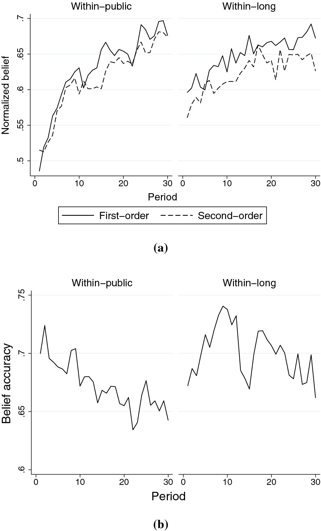
Fig. 10 The evolution of first- and second-order beliefs a and failure of higher-order learning b in the within-long treatment. Data from the within-public treatment are shown for comparison. In a, the beliefs are normalized by the correct state. In b, the accuracy of second-order beliefs is measured by

First-order beliefs in the within-long treatment are reported in the top panel of Fig. 10, with those in the within-public treatment also shown for comparison. In the first period, first-order beliefs in the within-long treatment are higher by 11 percentage points than those in the within-public treatment (
 ). On the other hand, first-order beliefs are not significantly different across these two treatments in period 30 (
 ). Overall, the pattern reported in Fig. 10 suggests that subjects take advantage of additional signals in the early rounds, but that there exists an upper bound on how much the average subject can learn about the state.Footnote 35
After 30 signals, first-order beliefs are less accurate in the within-long treatment than those in the within-public treatment. It is possible that this is driven by how the within-long treatment was implemented. As mentioned above, we presented subjects with 10 signals about the state of the world in each period of the within-long treatment.Footnote 36 Providing subjects with 10 signals at a time, as opposed to a sequence of 10 signals, might lead to underinference as discussed by Benjamin (Reference Benjamin2019, Sec. 4.2, Stylized Fact 2). On the other hand, the simulations, which do not assume bundling, point to an upper bound on first-order belief accuracy. Thus, the initial underinference in the within-long treatment might be driven by bundling, but the overall upper bound on belief accuracy is consistent with base-rate neglect.
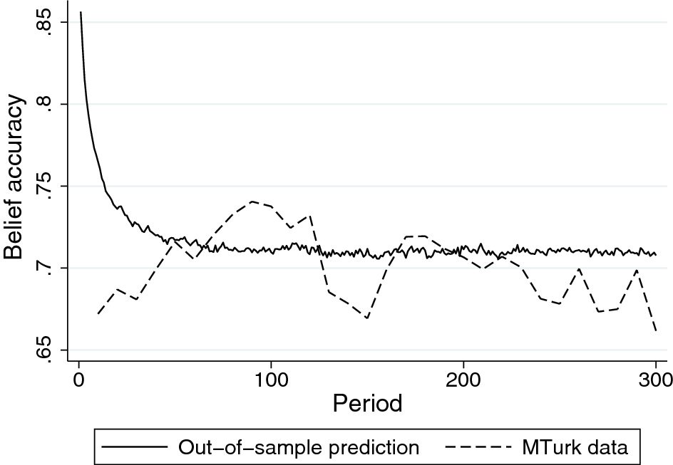
Fig. 11 Out of sample predicted accuracy of second-order beliefs together with the MTurk data in the within-long treatment. For the out of sample predictions, laboratory data from Player 2 in the public treatment is used. Belief accuracy is measured by

The average belief accuracy in the within-long treatment is plotted in the bottom panel of Fig. 10, with that in the within-public treatment again shown for comparison. Overall, we find that beliefs in the within-long treatment are more accurate than those in the within-public treatment, although the effect is only marginally significant (
 in a regression of the accuracy measure on a within-long dummy, using only the data from the within-public and within-long treatments). The magnitude of belief inaccuracy in the within-long treatment remains large. Moreover, beliefs in the last 15 periods of the within-long treatment are not more accurate than those in the first 15 periods (
 in a regression of the accuracy measure on a dummy variable for being in the last 15 rounds using only the data from the within-long treatment). This result is in line with Prediction Footnote 4.
The observed accuracy of second-order beliefs in the within-long treatment, together with the out of sample predictions described above, are shown together in Fig. 11. Overall, the data track the simulated predictions well. Taken together, the results in the within-long treatment suggest little benefit in terms of higher-order belief accuracy from receiving 300 as opposed to 30 public signals.
6 Conclusion
This paper presents the first experiment on how higher-order beliefs are updated in response to new information about the fundamentals. We find that subjects engage in higher-order thinking and shade their beliefs toward the prior when they receive private as opposed to public signals. On the other hand, we find that beliefs are not more accurate with public signals, contrary to the Bayesian prediction. Moreover, we find that beliefs do not become more accurate over time with either public or public signals, suggesting a failure of higher-order learning. We attribute this failure to base-rate neglect, heterogeneity in updating rules, and subjects’ failure to correctly model how other players deviate from Bayesian reasoning.
Failure of higher-order learning has implications for macroeconomic models. For instance, in a Calvo model with incomplete information about nominal shocks, Angeletos and La’O (Reference Angeletos and La‘O2009) show that knowledge about the evolution of first-order beliefs is insufficient to quantify the rate of price adjustment without taking into account the evolution of higher-order beliefs. In turn, higher-order beliefs affect firms’ forecasts of other firms’ equilibrium actions, which determine their own pricing choices. Our analysis shows that firms might have persistently incorrect beliefs about other firms’ beliefs about the size of a nominal shock. More importantly, sluggish price adjustments could persist even when firms in the economy observe only publicly available information.
Our investigation focuses attention on introspective learning where subjects do not receive feedback about the beliefs of others. This design choice guarantees that subjects’ higher-order beliefs are not simply the result of adaptation to the behavior of the matched partner. However, it also removes an important source of information which is often available in practice. An interesting extension would be to explore the evolution of higher-order beliefs in the presence of feedback about the average beliefs of a group of subjects to see whether the failure of higher-order learning that we observed could be reduced or even resolved. Noisy feedback, on the other hand, might generate a failure of higher-order learning similar to that we identify.
Acknowledgement
We are grateful to Ryan Oprea and seminar participants at the ESA World Meeting (Berlin) and the University of Southampton, the Editor, and two anonymous referees for very helpful comments. Financial support from the Asociación Mexicana de Cultura A.C., the Higher School of Economics, and the University of Surrey is acknowledged.
Appendix
A Implementation of the online treatments
For the within-public, within-private, and within-long treatments, the subject pool consisted of U.S. workers on Amazon Mechanical Turk (MTurk).Footnote 37 The data were collected using the software oTree (Chen et al., Reference Chen, Schonger and Wickens2016). Each subject was only allowed to participate in the experiment once, and the experiment was implemented through the assignment of MTurk qualifications to subjects that accepted the HIT (human intelligence task).
The data for the within-public treatment were collected separately as part of a different project. At the beginning of this treatment, subjects were administered a longer version of the Cognitive Reflection test (Frederick, Reference Frederick2005). The data for the within-long and within-private treatments were collected at the request of two referees and did not include any pre-experiment test.Footnote 38
In all the online treatments, each subject made a total of 60 decisions (30 guesses about the state and 30 guesses about the partner’s guess). The experiments’ framing was identical to that of the laboratory experiment. Each subject was paid on the basis of one randomly chosen decision out of 60 according to the Binarized Scoring rule with a bonus of $3.00 or nothing. The payment rule was clearly explained to the subjects in the instructions and several examples were provided, including a table indicating the loss corresponding to one’s choice and the different value of the target (the state of the world for the first decision, and the partner’s choice otherwise). Each decision screen summarized the most important information from the instructions, including a table of potential losses. The instructions and screenshots can be found in the online Appendix.
Subjects were shown the instructions for the experiment on their screens. After a subject finished reading the instructions, the subject waited to be matched. Given the possibility of no match occurring, subjects were asked to wait for at least up to five minutes for a match (no more than five minutes for within-long and within-private), after which they were allowed to quit (were terminated from) the study and collected their earnings up to that point plus a bonus to compensate the dismissed subjects for their time.Footnote 39 If two subjects were matched, the experiment automatically began. Each of the two per-period choices was presented on a separate screen and a subject had two minutes (one minute in the within-long and within-private treatments) to submit each choice.Footnote 40
B The dynamics of higher-order beliefs with private signals
Suppose that learning occurs through private signals. Let
 and
and
 denote the common prior belief that the state of the world is
 in period 0. Consider a binary signal technology with
 and
and

Since we are assuming that players are Bayesian expected utility maximizers and the signal technology is binary, a sufficient statistic for a history of length n observed by a player is the number of signals of type
 out of n total signals observed, which we denote by
 .
.
Let
 denote Player i’s posterior belief that the state is
 after having observed
 signals of type
 . By Bayes’ rule, this probability equals

Players 1, 2 and 3 form the same belief about the state of the world after having observed the same set of signals. Furthermore, if Player
 observed a history
 , and Player i knew which history Player
 observed, then Player i would assign probability one to Player
 assigning probability
 to state
 .
.
However, as learning occurs through private signals, players in higher-order roles need to form beliefs about the histories that players in lower-order roles might have observed. So, suppose that Player i observes history
 , she will use this information to update her beliefs about the state of the world which also informs her about the probability with which Player
 might have observed any feasible history. For any
 , Player i assigns probability
 to Player
 having observed
 signals of type
 in n draws when she observed
 such signals in n draws, this probability is given by

where, from the binomial distribution,

denotes the probability of observing
 signals of type
 out of n signals, conditional on state
 .
.
Given the incentives provided by the Binarized scoring rule in an arbitrary period n, Player 2 reports her expectation about the first-order beliefs held by Player 1 which is given by

We abuse notation slightly and write
 instead of
 to make explicit the fact that the beliefs are referenced to the state of the world being equal to
 .
.
Similarly, Player 3 reports her expectation about the report made by Player 2 which is given by

Next, we prove the following result:
Proposition B1
Suppose that the state of the world is
 and
and
 . Then, the following properties hold true:
a.
, for any
.b. For any
,
.


We split the proof into several steps. We first show two auxiliary results.
Lemma B1
For any
 ,
,
 .
.
Proof
Let
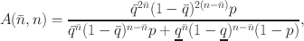
and notice that
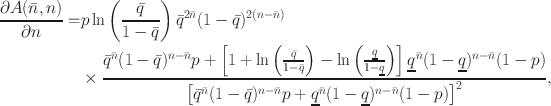
which is strictly positive and well-defined because
 . Then,
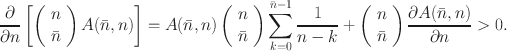
This implies that
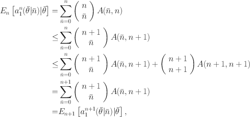
which completes the proof.

Lemma B2
 , for any
 .
.
Proof.
Note that, for any n > 0,
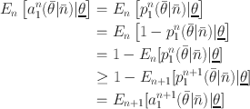
where the inequality follows from Lemma Footnote B1. Since

the result follows from the opposite monotonicity of the two sequences
 and
and
 .
.

We now prove part a) of the proposition.
Lemma B3
For any
 and
and
 ,
,
 .
.
Proof
Notice that
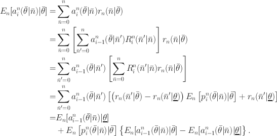
Then,

which is positive if and only if
 .Footnote 41 We know from Lemma Footnote B2 that this inequality holds for
 . So, suppose that it holds for
 , we will show that it also holds for
 . By equivalently expressing equation (17) in terms of
 instead of
 gives
gives
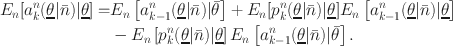
Next, given that the state space is binary, it holds that
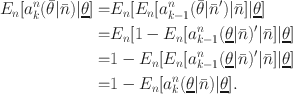
Combining (17) and (20), and rearranging using (20), we obtain
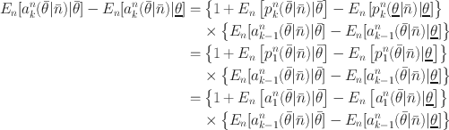
where the second equality follows from the observation that all players share the same first-order beliefs given the same history. Since
 by Lemma Footnote B2, and
 by the induction hypothesis, it follows that
 . Finally, this implies that
 , for any
 .
.

Next, we show part b) of the proposition. By Lemma Footnote B1, the sequence
 is monotonically increasing. As the sequence is also uniformly bounded above by 1, it converges. That
 follows from Markov’s inequality and a standard argument on the martingale property of Bayesian updating and is thus omitted. Similarly,
 . Therefore, from (17) with
 , we can conclude that
 . Using this fact and (17) again, we can show that the claim also holds for
 . This completes the proof.


 1-B
1-B
 λi
λi
 1-B
1-B

 1-|ait-a-i,t|

 1-B
1-B

 1-|ait-a-i,t|
 N=120
N=120 lnμn1-μn=β0+βPriorlnμn-11-μn-1+βLRln(LRn)+ϵ

 1-B
1-B
 1-|ait-a-i,t|
 1-|ait-a-i,t|


 Open access