Flip a coin or vote? An experiment on the implementation and efficiency of social choice mechanisms

Timo Hoffmann; Sander Renes

doi:10.1007/s10683-021-09724-9

Flip a coin or vote? An experiment on the implementation and efficiency of social choice mechanisms

Published online by Cambridge University Press: 14 March 2025

Timo Hoffmann and

Sander Renes

Show author details

Timo Hoffmann: Affiliation:
Chair of Economic Theory, Friedrich-Alexander Universität Erlangen-Nürnberg (FAU), Lange Gasse 20, 90403, Nürnberg, Germany
Sander Renes*: Affiliation:
Collaborative Research Center SFB 884 “Political Economy of Reforms”, Mannheim, Germany Erasmus School of Economics, Erasmus University Rotterdam, PO Box 1738, 3000 DR Rotterdam, The Netherlands
*: srenes@ese.eur.nl

Article contents

Abstract
Introduction
Related literature
Experimental design
Predictions
Results
Conclusion
Funding
Availability of data and material (data transparency)
Declarations
Footnotes
References

Rights & Permissions

Abstract

Corporate boards, experts panels, parliaments, cabinets, and even nations all take important decisions as a group. Selecting an efficient decision rule to aggregate individual opinions is paramount to the decision quality of these groups. In our experiment we measure revealed preferences over and efficiency of several important decision rules. Our results show that: (1) the efficiency of the theoretically optimal rule is not as robust as simple majority voting, and efficiency rankings in the lab can differ from theory; (2) participation constraints often hinder implementation of more efficient mechanisms; (3) these constraints are relaxed if the less efficient mechanism is risky; (4) participation preferences appear to be driven by realized rather than theoretic payoffs of the decision rules. These findings highlight the difficulty of relying on theory alone to predict what mechanism is better and acceptable to the participants in practice.

Keywords

Experimental economics Group choice Choice rules Mechanisms Participation constraints Individual rationality Two-stage voting Bayesian games Efficiency

JEL classification

C91: Laboratory, Individual Behavior D70: General C92: Laboratory, Group Behavior D82: Asymmetric and Private Information • Mechanism Design

Type: Original Paper
Information: Experimental Economics , Volume 25 , Issue 2 , April 2022 , pp. 624 - 655

DOI: https://doi.org/10.1007/s10683-021-09724-9 [Opens in a new window]
Creative Commons: This is an Open Access article, distributed under the terms of the Creative Commons Attribution (CC-BY) license (http://creativecommons.org/licenses/by/4.0/), which permits unrestricted re-use, distribution, and reproduction in any medium, provided the original work is properly cited.
Copyright: Copyright © The Author(s) 2021

1 Introduction

Before a group takes a decision—whether it is a corporate board thinking about investments, an expert panel considering different policies, a cabinet discussing reforms, or a nation considering who to appoint as president—the group has to select a decision rule that aggregates individual preferences into a group decision. With an inefficient decision rule, the group is likely to end up with less than optimal outcomes, e.g. bad investments, inefficient policies, unpopular presidential candidates, or simply deadlocked in discussions and forced to delay important decisions.Footnote ¹ If a group finds its existing decision rule does not work well, its members could choose to replace it. Therefore, it is natural to expect inefficient rules to be replaced. In practice, however, we regularly see inefficient decision rules persist. Examples range from veto rules or restricted voting rights that limit the amount of information combined in corporate boards and shareholder meetings (De Jong et al., Reference De Jong, DeJong, Mertens and Roosenboom2007; Grüner & Tröger, Reference Grüner and Tröger2019), mechanisms that are hindered by reputational concerns in expert panels (Visser & Swank, Reference Visser and Swank2007), the much criticized US electoral college (Rathbone, Reference Rathbone2018), and remarkably stable electoral systems despite changing circumstances (Rahat, Reference Rahat2011). In this paper, we use an experiment to shed more light on when we can expect inefficient decision rules to (not) be replaced by efficient ones.

To improve group decision rules, we need to take two necessary steps: design and implementation. First, we need to design and test an efficient mechanism for the particular context. Given the decisions at hand and the composition of the group, it might be better to use simple majority voting or to aim for group consensus. Second, we need to ensure that group members are willing to use the efficient mechanism. The corresponding design and participation problems have been studied extensively both theoretically and experimentally in the literature on exchange mechanisms such as auctions, matching, and market design. In contrast, the experimental part of the literature on efficient mechanisms in social choice is limited. The overview of the experimental literature presented in Chen (Reference Chen, Plott, Smith, Durlauf and Blume2008) only found one paper that analyzes the efficiency of the theoretically optimal mechanism (Attiyeh et al., Reference Attiyeh, Franciosi and Isaac2000). Similarly, tests of the participation decision only seem to have occurred in the class of voting rules (Engelmann & Grüner, Reference Engelmann and Grüner2017; Bol et al., Reference Bol, Blais, Coulombe, Laslier and Pilet2020; Engelmann et al., Reference Engelmann, Grüner, Hoffmann and Possajennikov2020).

Our paper addresses this gap in the literature on efficient social choice mechanisms in two ways. First, we use a revealed preference setup to measure subjects’ willingness to participate in several mechanisms that appear repeatedly in theory. Second, we measure and compare the empirical efficiency of these mechanisms. Together, the revealed preferences and achieved efficiency levels allow us to show how private information, expected benefits, and outside options—all difficult to observe outside the lab setting—influence participation preferences. Our experimental results thus shed light on the empirical efficiency and implementability of decision rules, both in a controlled lab environment.

Our results clearly show how outside options and private information shape subjects’ revealed preferences over mechanisms. Subjects that know they dislike the public project prefer a mechanism that does not allow provision but provides a safe payoff over all other mechanisms, as is predicted by the Myerson–Satterthwaite impossibility theorem (Myerson & Satterthwaite, Reference Myerson and Satterthwaite1983). Subjects who know they like the public project are willing to flip a coin to decide on the project as long as this increases the likelihood of implementation. Furthermore, both subjects that approve the public project and those that want to stop it prefer having influence over the outcome over flipping a coin. Therefore, with risky alternative mechanisms, voluntary participation in more efficient mechanisms can be possible even in ad interim stages, as is predicted by Schmitz (Reference Schmitz2002), Segal and Whinston (Reference Segal and Whinston2011) and Grüner and Koriyama (Reference Grüner and Koriyama2012). However, our results also show that the mechanisms are not as efficient in the lab as theory predicts, and the difference between theoretical predictions and measured efficiency depends on the setting and the mechanism. In some settings, the predicted ranking is reversed and therefore theoretical expectations of (individual) preferences for mechanisms can be misleading.

In our experiment, we study four mechanisms: the theoretical optimal Arrow-d’Aspremont–Gérard–Varet (AGV) mechanism,Footnote ² Simple Majority voting (SM), a Non-implementation mechanism that mimics the theoretical effects of forcing the Status Quo to persist by non-participation in the mechanism choice (NSQ), and flipping a coin (RAND, random decisions). The AGV mechanism is theoretically optimal in our public good setting. It is often used as the theoretical benchmark to which the efficiency other mechanisms are compared. However, the fact that the mechanism is optimal and efficient in theory does not necessarily translate to efficient outcomes in a laboratory or in practice. Despite its theoretical importance, the empirical performance of the AGV mechanism has not received much attention. To the best of our knowledge, the only direct test of its efficiency is in Attiyeh et al. (Reference Attiyeh, Franciosi and Isaac2000). They find that the AGV’s empirical efficiency is no larger than the theoretical efficiency of sincere voting in SM.Footnote ³ Our experiment allows us to directly compare AGV’s and SM’s achieved efficiency. The results show that the AGV mechanism is indeed more efficient than SM when the private valuations for the project are skewed. However, when the distribution is symmetric, SM is more efficient. We also show that SM is not as efficient as predicted in theory, but the difference between its predicted and achieved efficiency in the lab is much smaller and much more stable across settings than with the AGV. These findings highlight the importance of controlled tests for proposed mechanisms. Such tests are already the standard in auctions and matching (e.g. Roth, Reference Roth2012) and in the related setting of Voluntary Contribution Mechanisms (VCM) (e.g. Bracht et al., Reference Bracht, Figuieres and Ratto2008).Footnote ⁴

The differences between theoretical and achieved efficiency of the mechanisms, mean that our subjects’ preferences over mechanisms could be difficult to predict through theory alone. Remarkably, subjects can predict relative efficiency levels and select the mechanism that maximizes their expected payoff in the lab, even when the efficiency deviates from theoretic predictions. When SM is close to efficient, it is selected much more often than in settings where the AGV clearly outperforms SM in the lab. Furthermore, in a direct comparison, the empirical payoffs of the mechanisms more accurately predict mechanism choices than Bayes–Nash payoffs. Another difficulty of predicting the participation decisions and efficiency through theory alone, is the possibility that individuals attach value to non-monetary aspects. Group members that have other-regarding preferences attach a higher value to efficient mechanisms and might play differently within a given mechanism than narrowly self-interested group members (Engelmann & Grüner, Reference Engelmann and Grüner2017; Messer et al., Reference Messer, Poe, Rondeau, Schulze and Vossler2010; Bierbrauer et al., Reference Bierbrauer, Ockenfels, Pollak and Rückert2017). However, in our setting, where we cleanly identify participation decisions and see the play in the selected mechanisms, narrow self-interest is the most important predictor. In fact, subjects prefer complete randomness over arguably fairer and more efficient mechanisms, as long as randomness gives them a better chance to obtain their preferred outcomes.

The rest of the paper is organized as follows: Sect. 2 discusses related literature. Sect. 3 outlines the experimental design and treatments. Section 4 states the predictions we test, Sect. 5 tests these predictions and discusses further findings. Section 6 concludes.

2 Related literature

Our experiment is closely related to the literature on social choice and the choice of voting rules or constitutions. This literature is riddled with impossibility theorems that show the difficulties of designing a mechanism that combines a set of desirable properties. Most famously, Arrow (Reference Arrow1950) shows that non-dictatorship, Pareto efficiency, and independence of irrelevant alternatives cannot be obtained by any social choice rule for all potential preference profiles. In a similar vein, Myerson and Satterthwaite (Reference Myerson and Satterthwaite1983) show that with two players and independent valuations, an efficient, ad interim incentive-compatible and budget-neutral mechanism for trade does not exist as long as players are guaranteed a sufficiently large payoff when not trading.Footnote ⁵ Mailath and Postlewaite (Reference Mailath and Postlewaite1990) proof that individual rationality, incentive compatibility, and budget balance are also incompatible in an N-player public good setting like our experiment. Güth and Hellwig (Reference Güth and Hellwig1986, Reference Güth, Hellwig, Pethig and Schlieper1987) derive similar results for the private supply of a public good. In all these settings, it is impossible to achieve efficient production without a subsidy, if the mechanism choice is made through a veto rule (i.e. voluntary participation by all players). These impossibility results illustrate how participation constraints can stifle any chance of (efficient) mechanism change. For brevity, we will refer to this type of result as the Myerson–Satterthwaite impossibility theorem.

Our experiments recreate the conditions studied in several theoretic studies that show how (im-)possibility results depend on the relevant outside option. Cramton et al. (Reference Cramton, Gibbons and Klemperer1987) and Schmitz (Reference Schmitz2002) show that an interim status quo—either shared ownership or a probabilistic distribution of outcomes—can make it possible to design a mechanism that is both ad interim incentive compatible and ex post efficient, without requiring subsidies. Under independent and identically distributed private valuations, these results imply that one can always find a status quo mechanism that allows voluntary participation in the efficient mechanism ad interim, both for Myerson and Satterthwaite’s (Reference Myerson and Satterthwaite1983) bargaining game for the public good setting of our experiment. Segal and Whinston (Reference Segal and Whinston2011) make a similar point by demonstrating how background risk—a status quo that is not quite as secure as the no-trade outcome—can increase the willingness of individuals to accept mechanism changes. Their proposition 1 states that individuals are willing to accept an efficient mechanism if it has the same equilibrium distribution over allocations as the alternative mechanism. We recreate this risky alternative mechanism by flipping a coin in our experiment. Grüner and Koriyama (Reference Grüner and Koriyama2012) illustrate that in some cases it is even possible for groups to shift from a (simple) majority voting system to the AGV mechanism without violating interim participation constraints. Although SM is quite efficient in binary choice situations, the efficiency gains of the AGV are large enough to compensate individuals for the potential loss in information rents in some settings.

A few recent experimental papers have examined the choice for group decision rules over indivisible public goods. Weber (Reference Weber2017) compares the performance of two normative design rules, Penrose’s square root rule, and Shapley–Shubik power index in predicting subjects’ preference over voting rules in an indirect democracy. The interpretation of the ex ante stage also differs between our setting and Weber’s. In our setting, this stage refers to information about private payoffs of the decision, whereas in Weber’s setting it revolves about group membership, and private preferences are never known when making the mechanism choice.Footnote ⁶

Bierbrauer et al. (Reference Bierbrauer, Ockenfels, Pollak and Rückert2017) identify the theoretically optimal trade mechanism assuming players have other-regarding preferences. Their experiment shows that choices for a small but significant number of subjects are better explained by including other-regarding preferences. They also illustrate that if enough of such subjects are present, the social planner prefers a different mechanism than with narrowly self-interested agents. If social preferences play a role in our mechanisms, the theoretical predictions derived in models with narrowly self-interested agents might not hold.

The articles most closely related to ours are a small set of other experiments on mechanism choices for indivisible public goods. Engelmann and Grüner (Reference Engelmann and Grüner2017), Engelmann et al. (Reference Engelmann, Grüner, Hoffmann and Possajennikov2020) and Bol et al. (Reference Bol, Blais, Coulombe, Laslier and Pilet2020) also implement a two-stage group decision experiment for the provision of a public good. In Engelmann and Grüner’s (Reference Engelmann and Grüner2017) experiments, groups of five subjects select the number of votes required for implementation of the public good using a similar mechanism choice stage as our experiment. Narrowly self-interested, rational subjects always prefer the voting rule that requires only one (all five) vote(s) for implementation, if they have a positive (negative) valuation of the project. The same subjects should vote in favor of (against) implementation in the second stage to get their preferred outcome. However, subjects often choose intermediate thresholds (two, three, or four positive votes) indicating efficiency or prosocial concerns in the mechanism choice. A similar effect is found in Bol et al.’s (Reference Bol, Blais, Coulombe, Laslier and Pilet2020) experiments. Without information about private payoffs, the choice between the two voting mechanisms is strongly influenced by fairness concerns. In our experiments, ex post inequality is increased by AGV transfers in two treatments and decreased in another. However, our results do not indicate that the AGV is more attractive in the inequality reducing treatments. In Engelmann et al. (Reference Engelmann, Grüner, Hoffmann and Possajennikov2020), the focus is on the efficiency of the voting rule choices in the ex ante stage. They find that the ex ante mechanism choices are influenced by concerns related to the protection of strongly influenced minorities. The inefficiency in mechanism choices is found to cost more than one third of (theoretical) expected surplus on average. Our results indicate that this efficiency loss varies considerably depending on the setting.

Attiyeh et al. (Reference Attiyeh, Franciosi and Isaac2000) directly test the efficiency of the AGV. In their experiment, groups of five or ten subjects play a direct revelation game for the provision of a public good. Each subject randomly draws a private valuation between [ $- 10$ , 10] and can report any cent value in this range. Interestingly, the authors find that only about 10% of the reported preferences exactly match the private values, and this is mostly driven by one very honest subject. Almost all reports match the sign subjects’ preferences, indicating that many players tried to ’game the system’ despite its truthful Nash equilibrium. Unlike in our experiment, subjects in Attiyeh et al.’s (Reference Attiyeh, Franciosi and Isaac2000) experiment did not play any other mechanism so that these authors cannot compare the empirical efficiency of different mechanisms.

3 Experimental design

We first describe the game and the mechanisms used. We then describe the treatments and the procedures of the experiment. Treatments differ only in potential private valuations for the public project. The underlying procedures, game, and all other details of the experiment, e.g., number of rounds, group size, and available mechanisms, are identical across all treatments.

3.1 The game

Subjects interact in groups of three and each group decides whether or not to implement an indivisible public project. Each of the 18 experimental rounds consists of two stages. First, a mechanism is selected for each group. Second, the group decides about the implementation of the public project through the chosen mechanism. If the project is implemented, all players receive a project payoff equal to their private valuation. Non-implementation results in a zero payoff for all subjects.

At the beginning of a round, subjects are informed about the two available mechanisms. They cannot influence which mechanisms are available in a round, and the order of the comparisons is randomly altered between sessions. Each subject privately chooses one of the mechanisms. After the choices have been recorded, the computer randomly selects one group member as the dictator, and executes the mechanism chosen by this subject. The computer determines whether the project is implemented through the selected mechanism, and payoffs are realized accordingly. All group members are informed of the selected mechanism before they play it, but they do not learn whose choice was selected or what mechanism the other two subjects selected. At the end of the round subjects are informed about the outcome and payoffs for the period.

The random dictator elicitation for the mechanism choice clearly differs from the theoretical mechanism-design setting in two important ways. First, we force subjects to choose between two given mechanisms, rather than from all potential mechanisms. This binary choice set clearly identifies subjects’ outside option and allows us to manipulate it by changing the second mechanism. The drawback, a reduced choice set for participants, is unavoidable in any realistic empirical setting. Any other option would make identification of the outside option more difficult and would require subjects to choose between (infinitely) many mechanisms. Such choices are too demanding both on the experimental setup and for the subjects. Secondly, we follow the standard experimental methodology of randomizing the order of presentation in the mechanism choices rather than labeling one mechanism as the status quo or default. This randomization prevents response biases and thus allows a cleaner identification of preferences.

The experiment proceeds in two parts. In the first twelve rounds, subjects first choose their preferred mechanism in the ex ante stage and then learn their private valuation for the public project before the mechanism is played. In the last six rounds, subjects are informed about their private valuation for the project at the start of each round and therefore make mechanism choices in an ad interim stage. Subjects are never informed about the valuations of other subjects. Our subjects face all six possible binary mechanism choices twice in the ex ante condition (rounds 1–12), before going to the ad interim rounds (rounds 13–18).

The evaluation of efficiency requires a clean comparison between the mechanisms. In the ex ante rounds, the private valuations that determine the efficiency of the project can not influence the mechanism chosen and played. Furthermore, we ensure the choices in the ex ante rounds are not influenced by previous experiences in the ad interim rounds by running them at the start of the experiment. Therefore, we use the ex ante rounds to determine behavioral strategies and to calculate efficiency. We begin with two blocks of ex ante rounds to ensure we have enough observations with different combinations of private valuations for these calculations.

The design is in many respects similar to the two-stage voting procedure studied by Engelmann and Grüner (Reference Engelmann and Grüner2017) and Engelmann et al. (Reference Engelmann, Grüner, Hoffmann and Possajennikov2020), but there are three important differences. First, in our study subjects choose between two mechanisms rather than five. This clearly identifies the outside option. Second, we have four very different mechanisms, rather than five mechanisms from the class of simple voting rules. The mechanisms allow us to make the same comparisons studied in the theoretical papers cited above. We describe the mechanisms in the next subsection. Third, we vary the amount of private information possessed by participants, whereas the amount of information is kept constant in those experiments. Bol et al. (Reference Bol, Blais, Coulombe, Laslier and Pilet2020) also focus on the effects of private information but exclusively in relation to voting mechanisms and value-driven preferences. We focus on testing the implementability and efficiency of the SM and AVG in different settings and compare the outcomes with theoretical predictions. Value-driven preferences are found more often in similar settings to ours. We test for such social preferences/concerns in Sect. 5.2.

3.2 The four mechanisms

We chose the following four mechanisms because of their theoretical implications and relevance for group decision-making.

Mechanism I

AGV mechanism (AGV)

All group members report a valuation for the project. They can only report valuations that are present in the type space. If the sum of reported valuations is larger than zero, the project is implemented. If the sum is smaller than zero, the project is not implemented. Independent of project implementation, subjects pay or receive a transfer that depends on the vector of reported valuations.

Mechanism II

Voting—Simple Majority (SM)

All group members vote for or against the project (no abstention). If two or more group members vote for implementation, the project is implemented, otherwise the project is not implemented.

Mechanism III

Non-implementation Status Quo (NSQ)

The public project is not implemented.

Mechanism IV

Random implementation (RAND)

Whether the public project is implemented depends on the flip of a fair coin. The project is implemented with 50% probability independent of subjects’ valuations.

The AGV mechanism, or expected externality or pivot mechanism, is the theoretically optimal mechanism for decisions about indivisible public projects. It is incentive compatible, ex post budget balanced, and induces efficient implementation. It was first suggested by Arrow (Reference Arrow and Boskin1979) and d’Aspremont and Gérard-Varet (Reference d’Aspremont and Gérard-Varet1979) who also give a formal proof of its properties. The AGV is a direct revelation game in which all individuals send a message from the type space (they can behave like other types but cannot invent new types). The expected surplus generated by the project is calculated based on the reports, and the project is implemented if and only if the reported surplus is positive. If individuals report truthfully, this leads to efficient project implementation. To ensure truthful reports, the mechanism calls for transfers equal to the expected externality an individual generates for the others.Footnote ⁷ By including the externality in their payoffs, the mechanism forces individuals to take the expected surplus generated for the other players into account. As a result, all individuals are residual claimants of a value equal to the expected societal surplus they individually generate (their own surplus, plus the externality they impose on others). Consequently, they should send the message resulting in the highest expected social surplus. Since the AGV leads to first-best efficient implementation if all subjects report truthfully, this induces truthful reporting of all types. The AGV combines incentive compatibility with efficiency and budget balance and therefore the AGV provides the theoretical benchmark to which the performance of other mechanisms is compared. It is also an important benchmark for implementation. If it is impossible to switch from a given mechanism to the most efficient mechanism, the AGV, a switch to any other (less efficient) mechanism is unlikely.

The SM mechanism is chosen for two reasons. First, it is a common mechanism used in committee and small group decision-making and therefore provides a natural benchmark for the empirical performance of the AGV. Second, the comparison between AGV and SM is the focus of the possibility theorem in Grüner and Koriyama (Reference Grüner and Koriyama2012), such that we can use it to reproduce the theoretical choice setting of that paper. The NSQ mechanism resembles the opportunity for individuals not to take part in a decision process and thereby prevent a group decision. It mimics the non-participation option that causes Myerson–Satterthwaite impossibility. The RAND mechanism introduces an uncertain status quo and reproduces the comparisons with intermediate allocations as studied in Schmitz (Reference Schmitz2002) and Segal and Whinston (Reference Segal and Whinston2011).

3.3 Treatments

Treatments only differ in the distribution of private valuations for the public project. In all treatments, we use a uniform distribution over a type space with four possible valuations (in €) for the public project. The private valuations are drawn independently in each round. The distribution and its support are common knowledge and remain the same within a session.

The distribution of private valuations determines the expected payoff for the four mechanisms for each type. By varying the distributions, we thus vary the strength of the participation preferences over the mechanisms. For instance, theoretically AGV is always more efficient than SM, but the efficiency difference is much larger in skewed than in symmetric distributions. In the empirical analysis of the AGV, we find that subjects do not always truthfully reveal their private valuation. One suggested reason for such ’misreporting’, is that subjects mistake valuation reports with the same absolute value (report ’1’ rather than ’− 1’). This type of mistake is excluded in the Robustness treatment where the absolute value of the project valuation is unique for all types (Table 1).

Table 1 Distribution of valuations for the public project and number of observations by treatment

Treatment	Valuations (€)				Number of
Treatment	Valuations (€)				Subjects	Match groups
Symmetric	− 3	− 1	1	3	45	4
Right-skewed (+ 7)	− 3	− 1	1	7	42	4
Left-skewed (− 7)	− 7	− 1	1	3	45	5
Robustness	− 3	− 2	− 1	7	18	2
Probability	25%	25%	25%	25%

Probabilities are the same in all treatments. Subject types are drawn independently every round. A single treatment is used in each session

3.4 Procedures

The computerized experiments (zTree, Fischbacher, Reference Fischbacher2007) were conducted in the mLab of the University of Mannheim. Subjects were mostly undergraduate students from the University of Mannheim (recruitment through ORSEE, Greiner, Reference Greiner2015). Each session consisted of 18 rounds with random rematching of subjects in each matching group. In sessions with 18 or more participants there were two independent matching groups. All interactions were anonymous and subjects did not know who they were matched with in any round. To prevent income, effects only one randomly selected round was paid in addition to a show up fee of €9. Each round was equally likely to be chosen for payment and the selected round was identical for all subjects within a session. We conducted nine sessions with 6–24 subjects, resulting in 150 participants in 15 matching groups. Of these, 85 (57%) subjects were male and the average age of participants was 23. Sessions lasted just under an hour on average, the average payment was €9.40, with a minimum of €2 and a maximum of €16.Footnote ⁸

The 18 rounds were split into three six-round blocks: two blocks of ex ante rounds, followed by one block of ad interim rounds. Upon arrival in the lab, subjects received instructions for the first 12 rounds and were told about the existence of rounds 13–18. Subjects were only informed about the difference between rounds 1–12 and 13–18 (i.e., the revelation of private valuations before the mechanism choice in the ad interim rounds) after round 12. Subjects made each of the six possible binary mechanism choices once in each block, yielding three choices for each comparison. The order of the pairwise comparisons was randomized within each block and between sessions, and the order of the two mechanisms on subjects’ screens was randomized between blocks. Initially we also planned to run sessions with ad interim rounds before the ex ante rounds. However, since we found no indications of order effects in the mechanism choices but had extra questions regarding the reporting strategy in the AGV, we ran an extra session with the Robustness treatment instead. In the next section, we explain the theoretical predictions for all treatments.

4 Predictions

To derive the theoretical predictions, we have to make assumptions about the level of rationality and the preferences of our subjects. We start with Predictions Footnote 1.1–Footnote 1.4 that assume narrowly self-interested rationality, Prediction Footnote ² allows for non-selfish preferences, and Prediction Footnote ³ allows for non-Nash money maximization. Derivations of our predictions can be found in “Appendix A.1”.

4.1 Narrowly self-interested and full rational predictions

By definition, all subjects are equal at the ex ante stage, and thus the payoff-maximizing mechanism for each individual also maximizes the expected group surplus. In the ex ante rounds, a rational, risk-neutral, and purely self-interested agent considers the Bayes–Nash equilibrium of each mechanism and selects the mechanism with the highest efficiency. Table 2 below displays the preference ordering over mechanisms in the ex ante rounds for each treatment.

Since the AGV and SM mechanisms are more efficient than NSQ and RAND, without private information subjects should prefer AGV and SM over NSQ and RAND in all treatments. Similarly, ex ante they should prefer AGV over SM if Nash equilibrium is played. If there are deviations from equilibrium, the preferred mechanism can depend on the realized efficiency of the two mechanisms. We will return to this issue in Prediction Footnote ³ and Sect. 5.3.

Prediction 1.1

Without private information, all individuals prefer the more efficient of the two mechanisms in accordance with the ranking in Table 2.

Table 2 Predicted mechanism choices (ex ante)

Treatment	Ordering of mechanisms
Symmetric	AGV	$≻$	SM	$≻$	NSQ	$\sim$	RAND
Right-skewed (+ 7)	AGV	$≻$	SM	$≻$	RAND	$≻$	NSQ
Left-skewed (− 7)	AGV	$≻$	SM	$≻$	NSQ	$≻$	RAND
Robustness	AGV	$≻$	SM	$≻$	RAND	$≻$	NSQ

$≻$ and $\sim$ indicate the preference ordering of the four mechanisms for a risk-neutral subject. The ordering of mechanisms corresponds to their expected payoffs in the respective treatments. The payoff calculations for the AGV and SM assume truthful valuation reports (AGV) and sincere voting (SM), both in accordance with their respective Bayes–Nash equilibrium

In the ad interim rounds, subjects should consider the expected value of each mechanism given their valuation and the strategies played by other players. A complete list of all the preference rankings therefore entails 84 ( $4 \times 4 \times 6$ ) rankings between two mechanisms. The derivation of the following predictions and a table summarizing the 84 binary rankings can be found in “Appendix A.1”.

Theoretical work has identified several patterns in these binary rankings. Since the ranking of mechanisms depends directly on the valuation individuals have for the project, an individual with a negative valuation for the public project should choose the mechanism with the lowest implementation probability in Nash-equilibrium strategies. From this observation, we can conclude that the NSQ, with zero probability of implementation, dominates all other mechanisms for individuals with a negative project valuation. This is the application of the Myerson–Satterthwaite impossibility theorem in our setting: interim individual rationality makes all incentive compatible mechanisms less appealing than simply not participating for about half of our subjects.

Prediction 1.2

With private information, individuals with a negative valuation prefer NSQ to all other mechanisms.

Schmitz (Reference Schmitz2002) and Segal and Whinston (Reference Segal and Whinston2011) show that the impossibility in prediction Footnote 1.2 can be overcome if the outside option has a similar distribution over final outcomes as the efficient mechanism, rather than providing a safe payoff like NSQ. In our experiment, their results translate to the prediction that subjects should prefer AGV and SM over RAND even with private information.

Prediction 1.3

With private information:

1. all individuals prefer the AGV over the RAND mechanism;
2. all individuals prefer the SM over the RAND mechanism.

Grüner and Koriyama (Reference Grüner and Koriyama2012) demonstrate that individuals prefer the AGV over the SM as long as some conditions are met. In our experiment, their result translates to the following predictions:

Prediction 1.4

With private information subjects prefer the AGV over the SM if:

1. they have a private valuation of − 3 or + 3 in the Symmetric treatment;
2. they have a private valuation of 7 or 1 in the Right-skewed treatment;
3. they have a private valuation of − 7 or − 1 in the Left-skewed treatment;
4. they have a private valuation 7 or − 1 in the Robustness treatment.

4.2 Empirically derived predictions

Empirical observations show that Bayes–Nash predictions can and do fail in empirical tests, but some regularities can be found. Based on the empirical observations in various papers, we make two more predictions.

4.2.1 Social concerns

In Engelmann and Grüner (Reference Engelmann and Grüner2017), Bierbrauer et al. (Reference Bierbrauer, Ockenfels, Pollak and Rückert2017) and Bol et al. (Reference Bol, Blais, Coulombe, Laslier and Pilet2020) the authors show that social concerns impact mechanism choices. In the Right-skewed and Robustness treatment, the AGV transfers are pa id by subjects reporting high positive valuations. This “tax” thus reduces ex post inequality and increases the maximum payout to the type with lowest earnings without reducing the efficiency of the mechanism. In the Left-skewed treatment, a similar “tax” is levied from individuals with extremely negative valuations, increasing inequality. Thus, if we relax the assumptions on narrow self-interest and assume that utility increases in equality or the maxi-min criterion, the AGV should be more desirable in the Right-skewed and Robustness treatment than in the Left-skewed treatment. We expect this effect to be most visible in the ex ante rounds. In the ad interim rounds, we expect private benefits to dominate fairness concerns so that the later should not affect mechanism choices.

Prediction 2

1. The AGV mechanism is chosen more often in the Right-skewed and Robustness treatments than in the Left-skewed treatment.
2. This preference is more pronounced in the ex ante rounds than in the ad interim rounds.

4.2.2 Payoff maximization in the lab

Rational subjects are expected to maximize their own payoff within the experiment. However in the lab, the expected payoff of the SM and AGV mechanisms is not equal to their theoretical Nash-equilibrium payoff. Predictions about preferences over mechanisms based on Bayes–Nash equilibrium thus make incorrect assumptions and could incorrectly rank mechanisms. By varying the distribution of private valuations, we vary the payoff differences in the mechanism choice. This allows us to see if preferences over mechanisms indeed follow the payoff differences as expected. Furthermore, we expect the lab payoffs experienced by subjects to be better predictors of mechanism choices than theoretical Bayes–Nash equilibrium payoff.

Prediction 3

1. Mechanisms with a higher personal payoff are selected more often.
2. This relation is stronger for lab payoffs than for Bayes–Nash equilibrium payoffs.

5 Results

Before we look at the theoretical predictions about specific comparisons, we present an overview of the choice behavior over all treatments in Fig. 1.Footnote ⁹ We then present our results on each of the predictions. We compare the efficiency of AGV and SM when we test Prediction Footnote ³.

Fig. 1 Binary mechanism choices in the ex ante and the ad interim stage. Notes: Each of the six axes in the figures display the fraction of subjects choosing the mechanisms indicated at the corners. The scale of the diagonal axis can be read from both the vertical and horizontal axis. Separate sub-figures are drawn for choices in the ex ante rounds, the ad interim rounds with negative valuation, and ad interim rounds with positive valuation. Treatments are indicated by markers. The closer a marker is to a corner, the larger the fraction of subjects that chose that mechanism

In the summary overview of all binary choices in Fig. 1, we see some indications of the expected effects. In Fig. 1a, efficiency seems to matter in the ex ante mechanism choices. Subjects are close to indifferent between NSQ and RAND in the Symmetric and Robustness treatment where the ex ante expected value of implementation is (close to) zero, and more subjects favor NSQ (RAND) in the Left-skewed (Right-skewed) treatment that has a negative (positive) expected value. If we order the two treatments in terms of the relative efficiency of NSQ and RAND, we find the same order as on the lower axis of Fig. 1a. In line with Prediction Footnote 1.1, subjects overwhelmingly choose the more efficient, active mechanisms (SM and AGV) instead of the two passive ones. The choices between SM and AGV are close to the 50/50 distribution. SM is somewhat preferred in two treatments, whereas AGV is somewhat preferred in the Left-skewed treatment. In this last treatment, sending a message of − 7 acts as a veto, which could provide a clear limit to the risk this mechanism poses to subjects.

The ad interim choices in Fig. 1b also appear largely in line with expectations. Prediction Footnote 1.2 states that subjects with a negative valuation prefer NSQ (Myerson–Satterthwaite impossibility). This is clearly visible in the agglomeration of markings in the south-west corner of Fig. 1b in the negative valuation panel. This choice pattern is completely absent for subjects with a positive valuation, and can also not be found in the ex ante choices of the same subjects. Striking is also that this clustering on the inefficient mechanism only happens if the mechanism is safe (NSQ). In line with Prediction Footnote 1.3, subjects are much more likely to choose the SM or AGV over RAND, regardless of whether they have a positive or negative valuation.

Figure 1a shows that subjects prefer the AGV over SM most in the Left-skewed treatment. Whereas in the binary choice between NSQ and RAND no difference between treatments are found. This indicate that it is unlikely that Prediction Footnote ² will be supported by our data. The figure does not show much about the other predictions.

5.1 Theoretical predictions, Prediction 1

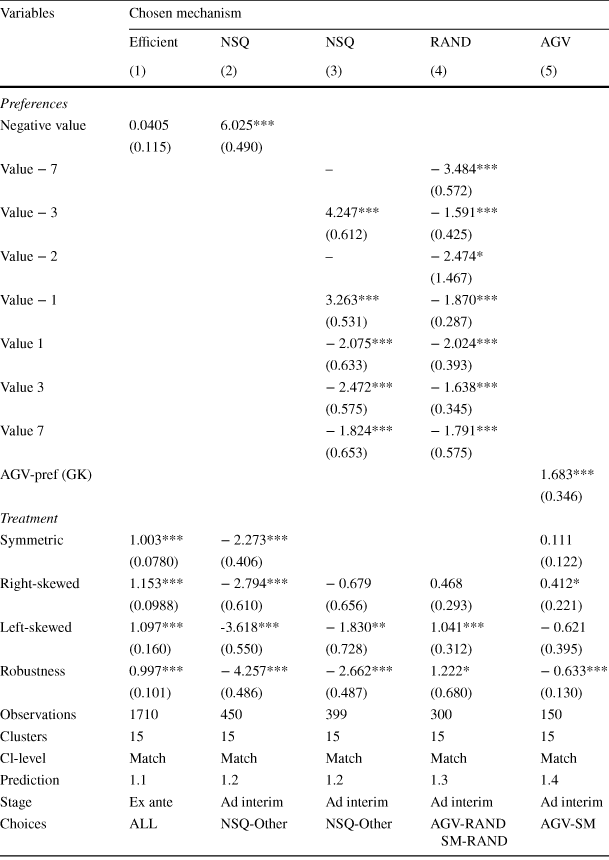
In Table 3, we use logistic regressions to test Predictions Footnote 1.1–Footnote 1.4. Throughout the paper, we cluster standard errors on the matching group (the largest group in the experiment that subjects could be matched with and thus could share some common history with) or treatment level and use a sandwich-estimator for the variance–covariance matrix based on Cameron et al. (Reference Cameron, Gelbach and Miller2012).

To test Prediction Footnote 1.1, we first define a dummy variable that is set to 1 if the subject selected the mechanism that is theoretically most efficient (we code the comparison RAND-NSQ as missing in the Symmetric treatment as these mechanism have the same expected efficiency). Column (1) shows that subjects indeed do not respond to the valuation before they know their valuation. More importantly, the coefficients on the full set of treatment dummies are positive and highly significant, indicating that subjects in every treatment prefer the efficient mechanism in the ex ante stage, as stated in Prediction Footnote 1.1.

Column (2) relates to Prediction Footnote 1.2. It shows ad interim subject-periods with a choice between NSQ and some other mechanism. As predicted by Myerson–Satterthwaite impossibility, subjects with a negative valuation are much more likely to choose the NSQ. The hypothesis that the sum of the treatment-specific constant and the coefficient on Negative Value is equal to zero is rejected in all treatments ( $χ^{2}$ -tests, $p < 0.001$ in all cases). Note the stark contrast with column (1) where both the treatment dummies and the Negative Value dummy have significantly smaller coefficient sizes. The Myerson–Satterthwaite theorem does not state that types with a negative value on average prefer NSQ, it states that all types with a negative valuation prefer the NSQ. Therefore, column (3) repeats the regression with a full set of valuation dummies (we drop the Symmetric treatment dummy for identification). The dummies for types $- 7$ and $- 2$ and corresponding observations are dropped because those types are perfectly predicted to select NSQ (see Fig. 1 and Online Appendix B.1.2). The coefficients on all negative valuations are positive and significant, whereas the coefficients on all positive valuations are negative and significant. Value $- 1$ is the marginal type in the type space and has the smallest positive coefficient. In $χ^{2}$ -tests against the restriction that the treatment dummies and the coefficient on Value $- 1$ add to zero, the null is rejected in all treatments (Right-skewed $p < 0.001$ , Left-skewed $p = 0.005$ , and Robustness $p = 0.039$ ). The pattern of Prediction Footnote 1.2 is clearly visible in the choices made by our subjects for all treatments and types.

In column (4), we look at the choice between flipping a coin or voting. Prediction Footnote 1.3 says that in these choices, all types should prefer AGV or SM to RAND. Indeed, we find that the coefficients on all types are negative and highly significant, indicating that RAND is not preferred. We repeat the $χ^{2}$ -tests on the sum of the treatment dummy and the smallest coefficient for a type present in that treatment. The Symmetric treatment is the baseline, so the coefficients measure the marginal effects and they are all significant and negative as predicted. In the Right-skewed treatment, $V a l u e - 3 + R i g h t k e w e d = 0$ yields $χ^{2} = 11.24$ , $p = < 0.001$ . In the Left-skewed treatment, $V a l u e 3 + L e f t - s k e w e d = 0$ yields $χ^{2} = 2.22$ , $p = < 0.1364$ . In the Robustness treatment, $V a l u e - 3 + R o b u s t n e s s = 0$ yields $χ^{2} = 0.27$ , $p = < 0.61$ . Over all treatments, the pattern of Prediction Footnote 1.3 appears visible. However, if we check on the individual-type level on which the prediction is made, we find null results in two treatments.

In column (5), we examine which types prefer AGV to SM. To have enough statistical power, we create a single dummy that identifies the types that Grüner and Koriyama (Reference Grüner and Koriyama2012) predict prefer the AGV over SM in the ad interim stage. The coefficient on the dummy AGV-pref (GK) is positive as predicted by Prediction Footnote 1.4 and is highly significant. Testing the restriction that the treatment dummies plus the coefficient AGV-pref (GK) equals zero yields: $χ^{2} = 52.78$ , $p = < 0.001$ in the Symmetric treatment; $χ^{2} = 31.45$ , $p = < 0.001$ in the Right-skewed treatment; $χ^{2} = 3.49$ , $p = < 0.06$ , in the Left-skewed treatment; $χ^{2} = 13.04$ , $p = < 0.001$ in the Robustness treatment. The pattern suggested by Prediction Footnote 1.4 is clearly identified over the treatments, but is only marginally significant in the Right-skewed treatment.

Table 3 Prediction 1, money-maximizing under full rationality

Variables	Chosen mechanism
	Efficient	NSQ	NSQ	RAND	AGV
	(1)	(2)	(3)	(4)	(5)
Preferences
Negative value	0.0405	6.025***
Negative value	(0.115)	(0.490)
Value − 7			–	− 3.484***
Value − 7				(0.572)
Value − 3			4.247***	− 1.591***
Value − 3			(0.612)	(0.425)
Value − 2			–	− 2.474*
Value − 2				(1.467)
Value − 1			3.263***	− 1.870***
Value − 1			(0.531)	(0.287)
Value 1			− 2.075***	− 2.024***
Value 1			(0.633)	(0.393)
Value 3			− 2.472***	− 1.638***
Value 3			(0.575)	(0.345)
Value 7			− 1.824***	− 1.791***
Value 7			(0.653)	(0.575)
AGV-pref (GK)					1.683***
AGV-pref (GK)					(0.346)
Treatment
Symmetric	1.003***	− 2.273***			0.111
Symmetric	(0.0780)	(0.406)			(0.122)
Right-skewed	1.153***	− 2.794***	− 0.679	0.468	0.412*
Right-skewed	(0.0988)	(0.610)	(0.656)	(0.293)	(0.221)
Left-skewed	1.097***	-3.618***	− 1.830**	1.041***	− 0.621
Left-skewed	(0.160)	(0.550)	(0.728)	(0.312)	(0.395)
Robustness	0.997***	− 4.257***	− 2.662***	1.222*	− 0.633***
Robustness	(0.101)	(0.486)	(0.487)	(0.680)	(0.130)
Observations	1710	450	399	300	150
Clusters	15	15	15	15	15
Cl-level	Match	Match	Match	Match	Match
Prediction	1.1	1.2	1.2	1.3	1.4
Stage	Ex ante	Ad interim	Ad interim	Ad interim	Ad interim
Choices	ALL	NSQ-Other	NSQ-Other	AGV-RAND SM-RAND	AGV-SM

Logistical regressions, dependent variables are dummies indicating that in a particular period this subject chose the indicated mechanism from the two available options. In column (4), two valuations and the 51 corresponding observations are not used in the regression because of colinearity issues and lack in variation, too many of the subjects with those types chose NSQ. Robust standard errors are in parentheses, *** $p < 0.01$ , ** $p < 0.05$ , * $p < 0.1$

The statistical noise we expect from our data asymmetrically affects theoretical predictions indicating implementation problems and potential solutions for two reasons. The first is directly observable in our data. In our statistical tests the problematic pattern of Prediction Footnote 1.2 is found very strongly. In fact, we have to drop some observations in column (3) because our statistics cannot deal with perfect identification. We do not see similarly strong patterns in the potential solutions to the impossibility in columns (4) and (5). In part, the fact that the later predictions are not as clear cut as the Myerson–Satterthwaite impossibility result is due to statistical power. We go from 1710 observation in 15 clusters in column (1) to only 150 observation in column (5). However, the theoretical predictions are made with certainty for all types, an expectation that is clearly not found in any real-world setting or the lab. Secondly, in many situations, we need all individual players or a qualified majority to accept a change in the rules. In a consensus or veto situation, we only need one opposing vote to prevent the implementation of efficient mechanisms. If we find a weak pattern in line with Prediction Footnote 1.2, this could be enough to prevent efficient mechanisms from being adopted. The opposite holds for Predictions Footnote 1.3 and Footnote 1.4. If we want the efficient mechanism to be voluntarily adopted, these predictions have to hold perfectly for all types. Any statistical noise around the prediction makes implementing efficient mechanisms more difficult. Since the results of these more qualified predictions are not as clear cut, empirical tests are needed to make sure such predictions are borne out in real life.

5.2 Social concerns, Prediction Footnote ²

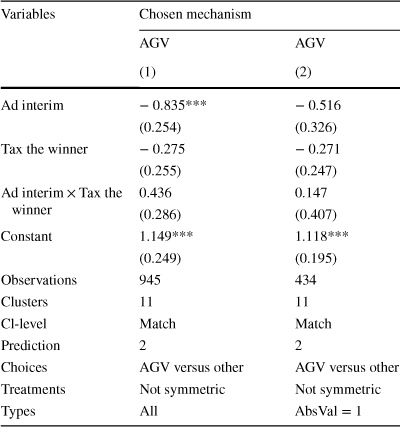
In the Right-skewed and Robustness (Left-skewed) treatments, the AGV transfers are paid by subjects that have a valuation of 7 (− 7) for the public project to subjects that have a negative (positive) valuation for the public project. These payments reduce (increase) ex post inequality after implementation of the project. Based on the results in Engelmann and Grüner (Reference Engelmann and Grüner2017), Bierbrauer et al. (Reference Bierbrauer, Ockenfels, Pollak and Rückert2017), and Bol et al. (Reference Bol, Blais, Coulombe, Laslier and Pilet2020) that subjects value fairness, we could expect subjects to prefer the AGV more in the Right-skewed treatment and Robustness treatment than in the Left-skewed treatment. In Table 4 we test this prediction by looking at the choices for AGV in a logistic regression with dummy Tax the winner set to 1 for the Right skewed and Robustness treatments, and to 0 for the Left-skewed treatment. We interact Tax the winner with a dummy indicating the ad interim rounds to see if the social concerns matter more ad interim or ex ante. In column (1), we look at all decisions of all types and see that, ad interim, the AGV is chosen less often than ex ante. The main effect and the interaction effect of the Tax the winner dummy are insignificant (and of opposing sign). Since the strength of preferences depend directly on the valuation for the public project, the types with extreme preferences could drive the null result. In column (2), we therefore repeat the analysis using only types with a valuation of − 1 or + 1. This does not change the sign or significance of the coefficients on Tax the winner. Contrary to Prediction Footnote ², there does not appear to be a prosocial tendency in the mechanism choices in our data.

Table 4 Effect of social concerns on mechanism choices

Variables	Chosen mechanism
	AGV	AGV
	(1)	(2)
Ad interim	− 0.835***	− 0.516
Ad interim	(0.254)	(0.326)
Tax the winner	− 0.275	− 0.271
Tax the winner	(0.255)	(0.247)
Ad interim $\times$ Tax the winner	0.436	0.147
Ad interim $\times$ Tax the winner	(0.286)	(0.407)
Constant	1.149***	1.118***
Constant	(0.249)	(0.195)
Observations	945	434
Clusters	11	11
Cl-level	Match	Match
Prediction	2	2
Choices	AGV versus other	AGV versus other
Treatments	Not symmetric	Not symmetric
Types	All	$AbsVal = 1$

Logistical regressions, dependent variables are dummies indicating that in a particular period this subject chose the indicated mechanism from the two available options. Robust standard errors in parentheses, *** $p < 0.01$ , ** $p < 0.05$ , * $p < 0.1$

The difference between our findings and those experiments that do find social concerns can be explained by a number of factors. For instance, subjects might not perceive enough difference in fairness between the mechanisms since they all have similar procedural fairness. Alternatively, the one-third probability that the mechanism choice has direct effects on the experiment, and thus on monetary payoffs, might overwhelm social concerns. The random, anonymous rematching used in this experiment restricts personal relations, dynamic strategies, and direct reciprocity, further reducing the potential for social concerns. Random rematching and random dictator choices clearly reduce the scope of the social concerns, but they are common in similar experiments that do find social concerns in group decision settings.Footnote ¹⁰ Our results thus put some bounds on the strength of these social concerns and/or the characteristics of the mechanisms that matter for the expression of social concerns by our subjects, but do not excluded social concerns per se.

5.3 Realized surplus, Prediction Footnote ³

Predictions Footnote 1.1–Footnote 1.4 assume that all subjects play Bayes–Nash strategies when determining the relative payoffs of the mechanisms. However, as we know from other experiments and experience, individuals seldom perfectly adhere to Bayes–Nash strategies, and realized payoffs of the mechanisms are an empirical matter. With different valuations, we should expect different rankings of mechanisms for an income maximizing subject. Prediction Footnote ³ focuses on these differences between theoretic and empirical payoffs and how these affect mechanism choice.

We compare the realized payoff for each mechanism based on the behavioral strategies and the objective probability over the vector of types, rather than the average surplus in the lab. The surplus obtained in the lab is strongly influenced by the realizations of private valuation and the mechanism choices by the random dictator which can distort the comparison. Therefore, we use the observed distribution of reports/votes made by subjects to determine behavioral strategies for each treatment-type. Using these behavioral strategies, we calculate the payoffs and surplus (in €) that would have realized in the limit where all combinations of private valuations occur with their expected probabilities. Equivalently, the realized surplus can be interpreted as the expected value of the next, unobserved round given these behavioral strategies.Footnote ¹¹

Table 5 Theoretical and realized group surplus with AGV and SM (ex ante)

Treatment	AGV			SM
	Group surplus			Group surplus
	Theory	Realized	Difference (%)	Theory	Realized	Difference (%)
Symmetric	1.59	1.18	− 0.41 (− 26%)	1.50	1.34	− 0.16 (− 11%)
Right-skewed (+ 7)	4.36	3.84	− 0.51 (− 12%)	3.75	3.68	− 0.07 (− 2%)
Left-skewed (− 7)	1.36	0.93	− 0.43 (− 32%)	0.75	0.66	− 0.09 (− 13%)
Robustness	3.28	2.93	− 0.35 (− 11%)	2.02	2.24	0.22 (11%)

Group surplus of an average round in Euro. Theoretical surplus is calculated based on Bayes–Nash equilibrium of the mechanisms. Realized surplus is based on behavioral strategies and can be interpreted as the expected value of the next round with this mechanism in the lab. The difference columns show by how much lab play differs from Nash equilibrium both in Euro and in percentages of theoretical surplus

Table 5 shows the Bayes–Nash surplus and the realized group surplus for the AGV and SM mechanisms in the ex ante rounds in all treatments.Footnote ¹² Neither mechanism reaches its full theoretical efficiency level. Still, SM is almost as efficient in the lab as predicted by theoretical calculations with rational, self-interested agents. The AGV is perfectly efficient in theory but loses a lot of its efficiency in practice. It is still the most efficient mechanism ex ante in the two Skewed treatments and the Robustness treatment. In the Symmetric treatment, SM is theoretically very close to optimal, which reduces the advantage of AGV in theoretic calculations. Simultaneously, the realized efficiency of AGV is quite low in this treatment, causing the realized efficiency ranking to reverse. The reversal of the efficiency ordering of AGV and SM makes it very difficult to predict preferences over mechanisms in the lab for subjects that are sensitive to realized payoff.

In every round, each group faces an efficient project (group surplus $> 0$ ) or inefficient project with the same probability. In the ex ante rounds, the efficiency of the project cannot affect the mechanism choices. Therefore, we compare the number of efficient and inefficient provision decisions (one decision per three matched subjects per period) in the ex ante rounds in Table 6. We choose this comparison over a comparison of the surplus in Table 5 for two reasons. The values in Table 6 are determined at the level of treatments, so that we only have one observation per treatment. Furthermore, the size and variance of the surplus varies over treatments because of the changes in the type space and in behavior, so that comparisons of the average surplus are not directly informative. Over the four treatments combined, implementation is marginally more efficient in the AGV. However, if we look at the results per treatment, the only difference found is in the Robustness treatment, whereas the SM is non-significantly more efficient in the Symmetric treatment. The Robustness treatment is the least Symmetric treatment, so exactly the situation where the theoretically expected difference between AGV and SM is largest. In Online Appendix B.2.4 we show that similar results are obtained through logistical regressions with clustered standard errors. The same appendix shows these null results are not purely due to lack of statistical power, as we can clearly show that the AGV has more efficient implementation than the extremely noisy RAND mechanism.

Table 6 Efficient implementation in the AGV and SM mechanisms

Treatment	All		Symmetric		Right-skewed		Left-skewed		Robustness
Treatment	AGV	SM	AGV	SM	AGV	SM	AGV	SM	AGV	SM
Inefficient	34	48	11	13	9	12	12	14	2	9
Efficient	189	164	50	62	53	48	62	38	24	16
Total	223	212	61	75	62	60	74	52	26	25
Odds ratio		0.615	1.049		0.681		0.528		0.15
Fisher-Exact, p-value		0.051	1		0.478		0.18		0.0188

Contingency table showing the numbers of efficient and inefficient project implementation decisions in the AGV and SM in each treatment. The lower part of the table shows the odds-ratio that compares the percentage of efficient implementation in both mechanisms as well as the corresponding p value from a two-sided Fisher’s exact test against the null of no difference between the mechanisms

Prediction Footnote ³ states subjects tend to select mechanisms with a higher expected payoff. After the ex ante rounds, subjects have experienced the mechanisms and thus have a feeling for the payoff they can obtain in the mechanisms in the lab. We create two proxies for these benefits by calculating the expected payoffs for each mechanism based on Bayes–Nash strategies and based on observed behavioral strategies for each treatment-type. We use the differences in expected utility between the two available mechanisms to explain the ad interim mechanism choices of each type in each treatment. This allows us to directly compare predictions based lab and Bayes–Nash payoffs for the second part of Prediction Footnote ³. Since strategies are determined at the treatment-type level, we aggregate our data to this level and determine the proportion of subjects with a given treatment-type that support mechanism A over mechanism B in a given choice.Footnote ¹³ This yields one observation per treatment-type and correlated errors within treatment since strategies are interdependent. We estimate a quasi-binomial model against the fraction of subjects that prefer the mechanism using both the theoretic and lab payoff differences as explanatory variables. We cluster standard errors on the treatment level. Since we want to examine the difference lab-based and theory-based predictions, we do not use the comparison between RAND and NSQ where the lab and theoretic payoffs are the same by construction. The results are shown in Table 7.

Table 7 Effect of utility differences on mechanism choice

	Proportion of support for mechanism A
	(1)	(2)	(3)
Utility difference lab	1.670***		1.203**
Utility difference lab	(0.572)		(0.572)
Utility difference theory		1.686***	0.528
Utility difference theory		(0.449)	(0.449)
Treatment 2	− 0.033	− 0.130***	− 0.056
Treatment 2	(0.042)	(0.042)	(0.042)
Treatment 3	− 0.333***	− 0.197***	− 0.292***
Treatment 3	(0.045)	(0.045)	(0.045)
Treatment 4	− 0.531***	− 0.400***	− 0.489***
Treatment 4	(0.037)	(0.037)	(0.037)
Constant	0.412***	0.243***	0.354***
Constant	(0.056)	(0.056)	(0.056)
Observations	79	79	79
Clusters	4	4	4
Cl-level	Treatment	Treatment	Treatment
Null deviance	47.97	47.97	47.97
Residual deviance	22.09	23.15	21.86
Prediction	3	3	3
Choices	AGV versus other,	AGV versus other	AGV versus other
Choices	SM versus other	SM versus other	SM versus other

Generalized linear model for fractional response (quasibinomial with logistic link function). The dependent variable is the fraction of subjects selecting a mechanism A from the two offered. The independent variables measure the difference in expected utility between mechanism A and mechanism B. Expected utility calculations are based on lab play in the first 12 rounds (Utility difference lab) or theoretic Bayes–Nash equilibria (Utility difference theory). Standard errors (in parentheses) are clustered on the treatment level and calculated through a sandwich procedure based on Cameron et al. (Reference Cameron, Gelbach and Miller2012). *** $p < 0.01$ , ** $p < 0.05$ , * $p < 0.1$

In columns (1) and (2), we estimate the model using the lab and theory measures of incentives, respectively. In both columns, types that gain more from the mechanism are more likely to select it ad interim. If we look at the overall model fit, we see a slightly better fit (lower residual deviance) for model (1) using lab predictions. In column (3), we pit the two predictors against each other directly. The positive correlation between the two independent variables decreases the coefficients’ sizes, but the lab-based measure is the only significant predictor. The model with both variables has a marginally better fit than both other models, but the difference is not statistically significant (Rao score test, theory only $p = 0.849$ , lab only $p = 0.937$ ). We looked at the ad interim rounds since we can see the choices made by each type individually there. We see something similar in the choice between AGV and SM in the ex ante rounds. In the Symmetric treatment, the realized surplus of the AGV is lower than that of SM in the lab. If we then look at Fig. 1a, we indeed see that support for the AGV is particularly low in that treatment. In fact, if we take the realized difference between AGV and SM in Table 5 and order the treatments accordingly, we find the exact same order as we see on the top axis of Fig. 1a. The expectations of Prediction Footnote ³ are clearly found in our data. The expected benefits of the mechanisms drive choices, and subjects respond most clearly to the expected benefits they experience in actual play.

The pattern of efficiency differences is interesting in its own right. Consistent with theory, the voting mechanism underperforms relative to the AGV particularly in situations with skewed distributions. The inability to show the intensity of preferences is particularly costly in these situations. However, the realized differences are very small and therefore difficult to notice in real life. These small differences can therefore create difficulties in the implementation of this more efficient mechanism.

Deviations from theoretical efficiency predictions stem from subjects’ second stage reporting (AGV) and voting (SM) strategies. Online Appendix B.2.1 shows that subjects that misreport the sign of their valuation in the AGV cause the largest loss in surplus. We show that the empirical best response of each type contains the truthful report and for most treatment-types it is unique. Reports with an incorrect sign could be caused by subjects that mistake $- 3$ for 3 or vice versa. We removed this possibility in the Robustness treatment, but we still find a significant number of misreported signs. Furthermore, we find a pattern where subjects with a positive valuation almost never misreport the sign of their valuation, whereas subjects with a negative valuation do so more often. As such, there appears to be a bias by some of our subjects in favor of implementing the public project in the lab. Interestingly, this asymmetric pattern is present in all treatments and across a number of individuals. In Online Appendix B.3, we look at how individual differences in reporting and voting strategies relate to personal characteristics. The most consistent effect we identify is that those individuals that are more likely to follow the Nash strategies of truthful revelation (sincere voting) are also most likely to select the AGV (SM) if given the option. This seems to imply that beliefs about the mechanisms influenced both selection of and play within the mechanisms. We find little evidence that the deviations from Nash equilibrium, either in the AGV or in SM, are driven by understanding of the experiment.

6 Conclusion

In group decision problems with conflicting interest, selecting an efficient decision rule is a problem characterized by conflict. The conflict over outcomes spills over to the mechanism selection stage and can make inefficient mechanisms persist. To allow groups to use more efficient mechanisms, we need to design mechanisms that are both more efficient and implementable in practice. This paper presents the results of one of the first experimental studies in a social choice setting that combines the dual aspects of practical efficiency and implementability.

In our experiment, the patterns found in mechanism choices are largely, but not completely, consistent with narrowly self-interested rationality. In line with predictions going back to Harsanyi (Reference Harsanyi1955), mechanism choices in an ex ante condition (behind-the-veil-of-ignorance) are efficient for the group. As the Myerson–Satterthwaite theorem and related impossibility results predict, the same subjects who prefer the theoretically optimal AGV ex ante, suddenly opt for the complete inertia of zero-implementation after learning their private valuation is negative. We also found the more qualified predictions of Schmitz (Reference Schmitz2002), Segal and Whinston (Reference Segal and Whinston2011) that subjects prefer AGV over flipping a coin (RAND) even after learning their private valuation, and that some types even prefer the AGV over SM ad interim (Grüner & Koriyama, Reference Grüner and Koriyama2012). However, theoretical predictions are not always accurate for all individual types or all possible situations. Not every subject prefers AGV over flipping a coin, and clear majorities for either AGV or SM often do not exist. Furthermore, a rational agent takes into account the realized payoff, including all deviations from Nash-equilibrium observed in reality. Since neither the optimal AGV nor SM are as efficient in the lab as in theory, theoretical predictions about the participation preferences of individuals are not always correct.

Our experiment highlights the difficulties of replacing a group decision rule with a more efficient one. This problem is fundamental to the socialist debate. It provides one possible answer to the question: “Why do centralized mechanisms like the state, and decentralized mechanisms like markets coexist?”. The difficulty to get even small groups with small stakes to accept efficient mechanisms, would translate to the near impossibility to get efficient mechanisms for a public project on the scale of a company, or nation (Mailath & Postlewaite, Reference Mailath and Postlewaite1990). Centralized organizations with coercive power, like states or companies, bundle decisions and projects and take the individual projects away from purely decentralized mechanisms like open markets. In our experiment, groups would have been better off if they would had forced to use the AGV or SM for all projects, rather than possibly having the zero-implementation NSQ whenever someone objected. Similarly, in society and in companies, the efficiency gains from joint investment in (a set of)common projects are often large enough to compensate participants for their involvement in some projects that are not individually rational to them. In the words of one of the classics in this debate (Clarke, Reference Clarke1971, p. 17): “If policing and exchange costs associated with a market arrangement are too high, substitute non-market devices may be preferred”.

The choices in our experiment confirm the effects of background risk on participation, as predicted by Schmitz (Reference Schmitz2002), Segal and Whinston (Reference Segal and Whinston2011), Grüner and Koriyama (Reference Grüner and Koriyama2012). This forces us to consider the outside options used in mechanism design. Simply equating the outside option to constant (zero) utility can affect behavior in the game through participation choices. When participation matters, equating the outside option to zero is more than just a normalization, it is a modeling choice that impacts the results.

Our setup allows us to vary individual participation constraints and compare subjects’ revealed preference for mechanisms before and after private information is received. We believe similar methods could be fruitfully applied to experimentally investigate other questions related to participation constraints, for instance in optimal auctions, monopoly pricing, or matching settings.

Acknowledgements

We appreciate the comments and the advice received (in alphabetical order) from Dirk Engelmann, Hans Peter Grüner, Eckhard Janeba, Henrik Orzen, Jeroen Suijs, Bauke Visser, as well as Lata Gangadharan [editor], Marie Claire Villeval [editor], and three anonymous reviewers. Furthermore, we appreciate the feedback of participants at the ESA conference in Heidelberg, the SEET meeting in Malta, the Bavarian Micro Day in Passau, the SABE conference in Wageningen, the Game Theory Society World Congress in Maastricht, the EEA meeting in Geneva and seminar participants in Mannheim, Nuremberg and Rotterdam. Financial support from the German research foundation (DFG), SFB 884 is gratefully acknowledged. All remaining errors are our own S. Renes, Raw data, the programs used to analyze the data, and the programs used to run the experiment are available from the EUR Data Repository under DOI: 10.25397/eur.14687301

Funding

Financial support from the German research foundation (DFG), via SFB 884 Political Economy of Reforms, is gratefully acknowledged.

Availability of data and material (data transparency)

Data and code used in analysis is available from the authors, and can be stored in journal’s repository if this is desirable.

Declarations

Conflicts of interest

Authors do not have any conflicts of interest to declare.

A Appendix

A.1 Derivation of predictions

A.1.1 Prediction Footnote 1.1

Note that all mechanisms generate as much surplus as is generated by the public project, as the rest of the (experimental) budget is ex post balanced. From the four mechanisms, the AGV mechanism is the only mechanism that implements (in Bayes–Nash equilibrium) the project if and only if the generated surplus is larger than 0. The other mechanisms all have an efficiency loss from wrong implementation, or wrong non-implementations and therefore are less efficient in expectation. These differences in efficiency imply the preference of individuals without private information for the AGV over NSQ and RAND mechanism in Prediction Footnote 1.1. The SM mechanism implements if and only if at least two people vote in favor. If we assume that individuals vote in favor if they have a positive valuation and against if it they have a negative valuation, we can see when the loss of efficiency in implementation occurs. In the Symmetric treatment this happens in two cases (type vectors ${- 1, - 1, 3}$ and ${1, 1, - 3}$ ), both of which cost 1€and occur with a probability of 4.6875%, such that the expected loss of the SM mechanism relative to first-best efficiency is 0.09€, or 5.88% of the maximum efficiency.

In the Right-skewed treatment with the + 7 value there are four cases of inefficient implementation, type vectors {− 3,− 3,7}, {− 3,− 1,7}, {− 3,1,1} and {− 1,− 1,7}, occurring with probabilities 4.6875%, 9.375%, 4.6875% and 4.6875% respectively. The expected loss is 0.61€, or 13.98% of maximum efficiency. In the Left-skewed treatment with the − 7 value there are four cases of inefficient implementation, type vectors {1,1,− 7}, {3,1,− 7}, {3,− 1,− 1} and {3,3,− 7}, occurring with probabilities 4.6875%, 9.375%, 4.6875% and 4.6875% respectively. The expected loss is also 0.61€, but this is 44.82% of maximum efficiency in this setting, since the maximum efficiency delivers a much lower surplus.

The RAND mechanism has a zero expected surplus for the Symmetric treatment, a €− 1 expected surplus in the Left-skewed treatment (€− 7), and a €1 expected surplus in the Right-skewed treatment (€7). The loss of efficiency of the NSQ is always 100%. Since the efficiency loss in the SM mechanism is always lower than the loss in the NSQ or RAND mechanism, this proves Prediction Footnote 1.1.

A.1.2 Prediction Footnote 1.2

With known private values $v_{i}$ , individuals can calculate their expected utility as a function of mechanism $Γ$ :

\begin{matrix} E (U) = v_{i} * Pr (Y = 1 | Γ = M) . \end{matrix}

With $Y = 1$ denoting implementation and $M \in$ {NSQ, RAND, SM}. With a negative private value, $v_{i}$ , the best response is to choose the mechanism with the lowest probability of implementation. Since $Pr (Y = 1 | Γ = NSQ) = 0$ , the NSQ (weakly) dominates {RAND, SM} for these individuals. For the AGV mechanism, we also have to verify that the transfers do not change this prediction. The expected transfer, in truth-telling Bayes–Nash equilibrium in the Symmetric treatment is − 0.125€ for the statements 3 and − 3 and + 0.125€ for − 1 and 1. For the AGV, the lowest implementation probability is achieved by any given subject by stating claiming the lowest type. Note, however, that this yields a probability of implementation that is strictly greater than 0 and a negative expected transfer, such that no rational individual with a negative valuation would choose this strategy over NSQ. Choosing AGV and playing claiming type -1 in the AGV yields an expected transfer of 0.13 [0.23] (0.23) € in the Symmetric [Left-skewed] (Right-skewed) treatment, but increases the implementation probability to 37.5% [37.5%] (50%) (assuming a truthful strategy of the other players). With any negative value, the expected implementation costs are therefore higher than the transfers. Since the transfers achieve their maximum at the − 1 report, while the probability of implementation keeps increasing in the reported valuation, this also rules out any strategy with a higher reported type. Hence, selecting the AGV and lying cannot be preferred to selecting NSQ. In fact, the expected transfers for types with a negative valuation are never large enough to change the preferences over mechanisms. A similar line of reasoning proves the same result for types with positive valuations.

A.1.3 Predictions Footnote 1.3 and Footnote 1.4

For the AGV, assume that individuals report truthfully in the second stage when playing AGV, and vote in favor in case of positive valuation and against otherwise in SM. Each individual should then choose the mechanism that maximizes her expected payoff, which for $M \in$ {NSQ, RAND, SM} is as before:

\begin{matrix} E (U) = v_{i} * P r (Y = 1 | Γ = M, v_{i}) . \end{matrix}

In the AGV the expected payoff is additionally influenced by the expected transfer each individual has to pay/receives, so it becomes:

\begin{matrix} E (U | A G V) = v_{i} * P r (Y = 1 | Γ = A G V, v_{i}) + E (t_{i} | m_{i} = v_{i}) . \end{matrix}

where $t_{i}$ is the transfer and $m_{i}$ the message send by the subject about her type. Since the individuals possess private information, this can be either positive or negative. It is straightforward, albeit somewhat tedious, to calculate the expected utility of each type for each of the three mechanisms in all treatments. The results are displayed in Table 8 below.

Table 8 Expected utility by type and mechanism in Bayes–Nash equilibrium

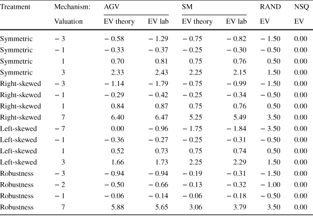
Treatment	Mechanism:	AGV		SM		RAND	NSQ
Treatment	Valuation	EV theory	EV lab	EV theory	EV lab	EV	EV
Symmetric	− 3	− 0.58	− 1.29	− 0.75	− 0.82	− 1.50	0.00
Symmetric	− 1	− 0.33	− 0.37	− 0.25	− 0.30	− 0.50	0.00
Symmetric	1	0.70	0.81	0.75	0.76	0.50	0.00
Symmetric	3	2.33	2.43	2.25	2.15	1.50	0.00
Right-skewed	− 3	− 1.14	− 1.79	− 0.75	− 0.99	− 1.50	0.00
Right-skewed	− 1	− 0.29	− 0.42	− 0.25	− 0.34	− 0.50	0.00
Right-skewed	1	0.84	0.87	0.75	0.76	0.50	0.00
Right-skewed	7	6.40	6.47	5.25	5.49	3.50	0.00
Left-skewed	− 7	0.00	− 0.96	− 1.75	− 1.84	− 3.50	0.00
Left-skewed	− 1	− 0.36	− 0.27	− 0.25	− 0.31	− 0.50	0.00
Left-skewed	1	0.52	0.73	0.75	0.74	0.50	0.00
Left-skewed	3	1.66	1.73	2.25	2.29	1.50	0.00
Robustness	− 3	− 0.94	− 0.94	− 0.19	− 0.31	− 1.50	0.00
Robustness	− 2	− 0.50	− 0.66	− 0.13	− 0.32	− 1.00	0.00
Robustness	− 1	− 0.06	− 0.14	− 0.06	− 0.18	− 0.50	0.00
Robustness	7	5.88	5.65	3.06	3.79	3.50	0.00

Expected value to a particular type in Euros for each treatment and types based on Bayes–Nash equilibrium strategy. Group surplus of an average round in Euro. The expected utility is based on Bayes–Nash equilibrium of the mechanisms

Like Segal and Whinston (Reference Segal and Whinston2016) showed more generally, no single type prefers to flip a coin over playing the AGV (or SM in this case). For the predictions of Grüner and Koriyama (Reference Grüner and Koriyama2012) we have a slightly more qualified result. In the skewed treatments the types − 3 and 3 prefer the SM mechanism, while all other types {− 7, − 1, 1, 7} prefer the AGV mechanism. In the Symmetric treatment the types − 1 and 1 are indifferent, while the types − 3 and 3 prefer AGV.

A.1.4 Preference ranking ad interim, full rationality and narrowly self-interested

Table 9 shows the order of the expected payoffs in the ad interim rounds per treatment and valuation, assuming the Bayes–Nash equilibrium is played.

Table 9 Predicted mechanism choices (ad interim)

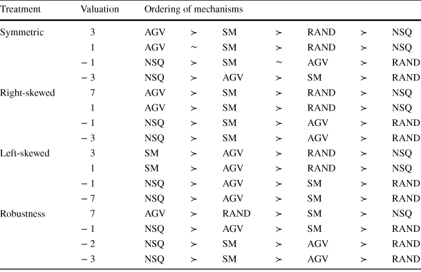
Treatment	Valuation	Ordering of mechanisms
Symmetric	3	AGV	$≻$	SM	$≻$	RAND	$≻$	NSQ
	1	AGV	$\sim$	SM	$≻$	RAND	$≻$	NSQ
	− 1	NSQ	$≻$	SM	$\sim$	AGV	$≻$	RAND
	− 3	NSQ	$≻$	AGV	$≻$	SM	$≻$	RAND
Right-skewed	7	AGV	$≻$	SM	$≻$	RAND	$≻$	NSQ
	1	AGV	$≻$	SM	$≻$	RAND	$≻$	NSQ
	− 1	NSQ	$≻$	SM	$≻$	AGV	$≻$	RAND
	− 3	NSQ	$≻$	SM	$≻$	AGV	$≻$	RAND
Left-skewed	3	SM	$≻$	AGV	$≻$	RAND	$≻$	NSQ
	1	SM	$≻$	AGV	$≻$	RAND	$≻$	NSQ
	− 1	NSQ	$≻$	AGV	$≻$	SM	$≻$	RAND
	− 7	NSQ	$≻$	AGV	$≻$	SM	$≻$	RAND
Robustness	7	AGV	$≻$	RAND	$≻$	SM	$≻$	NSQ
	− 1	NSQ	$≻$	AGV	$≻$	SM	$≻$	RAND
	− 2	NSQ	$≻$	SM	$≻$	AGV	$≻$	RAND
	− 3	NSQ	$≻$	SM	$≻$	AGV	$≻$	RAND

$≻$ and $\sim$ indicate the preferences ordering of the four mechanisms for a risk-neutral subject. The ordering of mechanisms corresponds to their expected payoffs given the respective treatment and valuation

Footnotes

Supplementary Information The online version contains supplementary material available at https://doi.org/10.1007/s10683-021-09724-9.

¹ In our experiment all mechanisms are group decision and we use these terms interchangeably. For discussions and examples of the decision rules in the settings mentioned, see for instance: Malenko (Reference Malenko2014), Gao and Huang (Reference Gao and Huang2018) about corporate boards; Swank et al. (Reference Swank, Swank and Visser2008), Hao and Suen (Reference Hao and Suen2009) about (expert) policy committees; and Colomer (Reference Colomer and Colomer2004), Benoit (Reference Benoit2007), Goux and Hopkins (Reference Goux and Hopkins2008), Widgrén (Reference Widgrén2009), Warntjen (Reference Warntjen2010) for political examples.

² The original mechanism was derived in Arrow (Reference Arrow and Boskin1979) and d’Aspremont and Gérard-Varet (Reference d’Aspremont and Gérard-Varet1979). In our setting, the mechanism is part of the class of Vickrey–Clarke–Groves mechanisms that were derived from foundational work by Vickrey (Reference Vickrey1961), Clarke (Reference Clarke1971), Groves (Reference Groves1973). It is also known as the expected externality mechanism, or pivot mechanism (Tideman & Tullock, Reference Tideman and Tullock1976).

³ Several follow-up papers have examined possibilities to improve the empirical performance of mechanisms like the AGV, but do not compare the AGV to more empirically relevant mechanisms (Kawagoe & Mori, Reference Kawagoe and Mori2001; Cason et al., Reference Cason, Saijo, Sjöström and Yamato2006).

⁴ This literature is too large to survey here. Numerous contributions can be found in collections like Plott (Reference Plott2008), Kagel and Roth (Reference Kagel and Roth1997, Reference Kagel and Roth2016). The difference between stylized theory and chaotic practice has caused the literature on market design to use an ever more integrated approach combining theory and experiments (Roth, Reference Roth2012, Reference Roth2015). In the related setting of the provision of divisible public goods, a similar literature has developed around (improvements to) VCM. For instance, Falkinger et al. (Reference Falkinger, Fehr, Gächter and Winter-Ember2000) test one such mechanism against the normal VCM, and Hamman et al. (Reference Hamman, Weber and Woon2011) examine mechanism choice in the VCM setting.

⁵ An older, less general result can be found in Chatterjee (Reference Chatterjee1982), and a more general statement of this result can be found in e.g. Segal and Whinston (Reference Segal and Whinston2016). The interpretation in this paper is mostly due to Cramton et al. (Reference Cramton, Gibbons and Klemperer1987).

⁶ The ex ante stage is often referred to as ’behind the veil-of-ignorance’ in reference to Harsanyi (Reference Harsanyi1955) and Rawls (Reference Rawls1971). However, the definition of behind-the-veil differs depending on the setting. In this paper we therefore use ex ante and ad interim when talking about private information for clarity.

⁷ The translated instructions for the Symmetric treatment in Online Appendix C include a table of all possible transfers.

⁸ Per treatment the average [minimum–maximum] payments were, Symmetric treatment €9.27 [5.75–12.00]; Right-skewed treatment €9.79 [5.16–16.00]; Left-skewed treatment €8.71 [2.00–11.96]; Robustness treatment €10.5 [6.00–16.00]. The translated instructions for the Symmetric treatment and screen shots from the original zTree program can be found in Online Appendix C.

⁹ Online Appendix B.1 shows a more detailed breakdown of all mechanism choices.

¹⁰ See for instance Feddersen et al. (Reference Feddersen, Gailmard and Sandroni2009), Botelho et al. (Reference Botelho, Harrison, Pinto and Rutström2005), Engelmann and Grüner (Reference Engelmann and Grüner2017), Bierbrauer et al. (Reference Bierbrauer, Ockenfels, Pollak and Rückert2017), or Bol et al. (Reference Bol, Blais, Coulombe, Laslier and Pilet2020).

¹¹ The calculations involve a direct comparison of the efficiency of AGV and SM on the same group of subjects. This comparison can be of independent interest for mechanism design in social choice. We therefore analyze the realized efficiency of these mechanisms in more detail in Online Appendix B.2. In this appendix we also show a table with the average payoff realized in the lab without correcting for the random draws in the experiment.

¹² We concentrate on the ex ante rounds because in these rounds the private valuations, and thus the efficiency of the mechanisms, cannot influence the mechanisms played. Although they are noisier, results for the ad interim rounds are qualitatively similar.

¹³ Mechanism A is defined as the AGV if available, or the SM mechanism otherwise. Online Appendix B.1.3 graphically displays the data and GLM model fit.

Springer Nature remains neutral with regard to jurisdictional claims in published maps and institutional affiliations.

References

Arrow, K (1950). A difficulty in the concept of social welfare. The Journal of Political Economy, 58(4), 328–346. 10.1086/256963CrossRef Google Scholar

Arrow, K, & Boskin, MJ (1979). The property rights doctrine and demand revelation under incomplete information. Economics and human welfare, New York Academic Press 23–39. 10.1016/B978-0-12-118850-4.50007-2CrossRef Google Scholar

Attiyeh, G, Franciosi, R, & Isaac, RM (2000). Experiments with the pivot process for providing public goods. Public Choice, 102(1–2), 93–112. 10.1023/A:1005025416722CrossRef Google Scholar

Benoit, K (2007). Electoral laws as political consequences: Explaining the origins and change of electoral institutions. Annual Review of Political Science, 10, 363–390. 10.1146/annurev.polisci.10.072805.101608CrossRef Google Scholar

Bierbrauer, F, Ockenfels, A, Pollak, A, & Rückert, D (2017). Robust mechanism design and social preferences. Journal of Public Economics, 149, 59–80. 10.1016/j.jpubeco.2017.03.003CrossRef Google Scholar

Bol, D., Blais, A., Coulombe, M., Laslier, J.-F., & Pilet, J.-B. (2020). Choosing an electoral rule. SocArXiv Working Paper rm2tq, Center for Open Science.Google Scholar

Botelho, A., Harrison, G. W., Pinto, L., & Rutström, E. E. (2005). Social norms and social choice. Working Paper 30, University of Minho. Nucleus of Research in Applied Microeconomics (NIMA).Google Scholar

Bracht, J, Figuieres, C, & Ratto, M (2008). Relative performance of two simple incentive mechanisms in a public goods experiment. Journal of Public Economics, 92(1–2), 54–90. 10.1016/j.jpubeco.2007.04.005CrossRef Google Scholar

Cameron, AC, Gelbach, JB, & Miller, DL (2012). Robust inference with multiway clustering. Journal of Business and Economic Statistics, 29(2), 238–249. 10.1198/jbes.2010.07136CrossRef Google Scholar

Cason, TN, Saijo, T, Sjöström, T, & Yamato, T (2006). Secure implementation experiments: Do strategy-proof mechanisms really work?. Games and Economic Behavior, 57(2), 206–235. 10.1016/j.geb.2005.12.007CrossRef Google Scholar

Chatterjee, K (1982). Incentive compatibility in bargaining under uncertainty. The Quarterly Journal of Economics, 97(4), 717–726. 10.2307/1885109CrossRef Google Scholar

Chen, Y Plott, CR, Smith, SN, Durlauf, VL, & Blume, LE (2008). Incentive-compatible mechanisms for pure public goods: A survey of experimental research. Handbook of experimental economics results, Elsevier 625–643. 10.1016/S1574-0722(07)00067-4CrossRef Google Scholar

Clarke, EH (1971). Multipart pricing of public goods. Public Choice, 11(1), 17–33. 10.1007/BF01726210CrossRef Google Scholar

Colomer, JM, & Colomer, JM (2004). The strategy and history of electoral system choice. The handbook of electoral system choice, Springer 3–78. 10.1057/9780230522749_1CrossRef Google Scholar

Cramton, P, Gibbons, R, & Klemperer, P (1987). Dissolving a partnership efficiently. Econometrica, 55(3), 615–632. 10.2307/1913602CrossRef Google Scholar

d’Aspremont, C, & Gérard-Varet, L-A (1979). Incentives and incomplete information. Journal of Public Economics, 11(1), 25–45. 10.1016/0047-2727(79)90043-4CrossRef Google Scholar

De Jong, A, DeJong, DV, Mertens, G, & Roosenboom, P (2007). Investor relations, reputational bonding, and corporate governance: The case of royal ahold. Journal of Accounting and Public Policy, 26(3), 328–375. 10.1016/j.jaccpubpol.2007.03.002CrossRef Google Scholar

Engelmann, D., & Grüner, H. P. (2017). Tailored Bayesian mechanisms: Experimental evidence from two-stage voting games. CESifo Working Paper Series 6405, CESifo.CrossRef Google Scholar

Engelmann, D., Grüner, H. P., Hoffmann, T., & Possajennikov, A. (2020). Minority protection in voting mechanisms-experimental evidence. CEPR Discussion Paper DP14393, CEPR.Google Scholar

Falkinger, J, Fehr, E, Gächter, S, & Winter-Ember, R (2000). A simple mechanism for the efficient provision of public goods: Experimental evidence. American Economic Review, 90(1), 247–264. 10.1257/aer.90.1.247CrossRef Google Scholar

Feddersen, T, Gailmard, S, & Sandroni, A (2009). Moral bias in large elections: Theory and experimental evidence. American Political Science Review, 103(2), 175–192. 10.1017/S0003055409090224CrossRef Google Scholar

Fischbacher, U (2007). z-tree: Zurich toolbox for ready-made economic experiments. Experimental Economics, 10(2), 171–178. 10.1007/s10683-006-9159-4CrossRef Google Scholar

Gao, H, & Huang, J (2018). The even–odd nature of audit committees and corporate earnings quality. Journal of Accounting, Auditing and Finance, 33(1), 98–122. 10.1177/0148558X15625438CrossRef Google Scholar

Goux, DJ, & Hopkins, DA (2008). The empirical implications of electoral college reform. American Politics Research, 36(6), 857–879. 10.1177/1532673X08324213CrossRef Google Scholar

Greiner, B (2015). Subject pool recruitment procedures: Organizing experiments with ORSEE. Journal of the Economic Science Association, 1(1), 114–125. 10.1007/s40881-015-0004-4CrossRef Google Scholar

Groves, T (1973). Incentives in teams. Econometrica, 41(4), 617–631. 10.2307/1914085CrossRef Google Scholar

Grüner, HP, & Koriyama, Y (2012). Public goods, participation constraints, and democracy: A possibility theorem. Games and Economic Behavior, 75(1), 152–167. 10.1016/j.geb.2011.11.001CrossRef Google Scholar

Grüner, HP, & Tröger, T (2019). Linear voting rules. Econometrica, 87(6), 2037–2077. 10.3982/ECTA16004CrossRef Google Scholar

Güth, W, & Hellwig, M (1986). The private supply of a public good. Journal of Economics, 5, 121–159. 10.1007/BF03051789CrossRef Google Scholar

Güth, W, Hellwig, M Pethig, R, & Schlieper, U (1987). Competition versus monopoly in the supply of public goods. Efficiency, institutions and economic policy, Springer 183–217. 10.1007/978-3-642-73064-1_17CrossRef Google Scholar

Hamman, JR, Weber, RA, & Woon, J (2011). An experimental investigation of electoral delegation and the provision of public goods. American Journal of Political Science, 55(4), 738–752. 10.1111/j.1540-5907.2011.00531.xCrossRef Google Scholar

Hao, L, & Suen, W (2009). Decision-making in committees. Canadian Journal of Economics/Revue Canadienne d’économique, 42(2), 359–392. 10.1111/j.1540-5982.2009.01512.xCrossRef Google Scholar

Harsanyi, JC (1955). Cardinal welfare, individualistic ethics, and interpersonal comparisons of utility. Journal of political Economy, 63(4), 309–321. 10.1086/257678CrossRef Google Scholar

Kagel, JH, & Roth, AE (1997). The handbook of experimental economics, Princeton University Press.Google Scholar

Kagel, JH, & Roth, AE (2016). The handbook of experimental economics, Princeton University Press.Google Scholar

Kawagoe, T, & Mori, T (2001). Can the pivotal mechanism induce truth-telling? An experimental study. Public Choice, 108(3–4), 331–354. 10.1023/A:1017542406848CrossRef Google Scholar

Mailath, G, & Postlewaite, A (1990). Asymmetric information bargaining problems with many agents. The Review of Economic Studies, 57(3), 351–367. 10.2307/2298018CrossRef Google Scholar

Malenko, N (2014). Communication and decision-making in corporate boards. The Review of Financial Studies, 27(5), 1486–1532. 10.1093/rfs/hht075CrossRef Google Scholar

Messer, KD, Poe, GL, Rondeau, D, Schulze, WD, & Vossler, CA (2010). Social preferences and voting: An exploration using a novel preference revealing mechanism. Journal of Public Economics, 94(3–4), 308–317. 10.1016/j.jpubeco.2009.12.004CrossRef Google Scholar

Myerson, R, & Satterthwaite, M (1983). Efficient mechanisms for bilateral trading. Journal of Economic Theory, 29(2), 265–281. 10.1016/0022-0531(83)90048-0CrossRef Google Scholar

Plott, C (2008). Handbook of experimental economics results, Elsevier.Google Scholar

Rahat, G (2011). The politics of electoral reform: The state of research. Journal of Elections, Public Opinion & Parties, 21(4), 523–543. 10.1080/17457289.2011.609618CrossRef Google Scholar

Rathbone, M (2018). Reform of the electoral college. Political Insight, 9(4), 16–19. 10.1177/2041905818815192CrossRef Google Scholar

Rawls, J (1971). A theory of justice, Harvard University Press 10.4159/9780674042605CrossRef Google Scholar

Roth, A. E. (2012). The theory and practice of market design. https://www.nobelprize.org/prizes/economic-sciences/2012/roth/lecture/. Online; Accessed 09 June 2021.Google Scholar

Roth, AE (2015). Who gets what–and why: The new economics of matchmaking and market design, Houghton Mifflin Harcourt.Google Scholar

Schmitz, P (2002). Simple contracts, renegotiation under asymmetric information, and the hold-up problem. European Economic Review, 46(1), 169–188. 10.1016/S0014-2921(01)00088-5CrossRef Google Scholar

Segal, I, & Whinston, M (2011). A simple status quo that ensures participation (with application to efficient bargaining). Theoretical Economics, 6(1), 109–125. 10.3982/TE591CrossRef Google Scholar

Segal, I, & Whinston, MD (2016). Property rights and the efficiency of bargaining. Journal of the European Economic Association, 14(6), 1287–1328. 10.1111/jeea.12185CrossRef Google Scholar

Swank, J, Swank, OH, & Visser, B (2008). How committees of experts interact with the outside world: Some theory, and evidence from the FOMC. Journal of the European Economic Association, 6(2–3), 478–486. 10.1162/JEEA.2008.6.2-3.478CrossRef Google Scholar

Tideman, TN, & Tullock, G (1976). A new and superior process for making social choices. Journal of Political Economy, 84(6), 1145–1159. 10.1086/260505CrossRef Google Scholar

Vickrey, W (1961). Counterspeculation, auctions, and competitive sealed tenders. The Journal of Finance, 16(1), 8–37. 10.1111/j.1540-6261.1961.tb02789.xCrossRef Google Scholar

Visser, B, & Swank, OH (2007). On committees of experts. The Quarterly Journal of Economics, 122(1), 337–372. 10.1162/qjec.122.1.337CrossRef Google Scholar

Warntjen, A (2010). Between bargaining and deliberation: Decision-making in the Council of the European Union. Journal of European Public Policy, 17(5), 665–679. 10.1080/13501761003748641CrossRef Google Scholar

Weber, M (2017). Choosing the rules: Preferences over voting systems for assemblies of representatives. Journal of Economic Behavior and Organization, 174, 420–434. 10.1016/j.jebo.2017.01.016CrossRef Google Scholar

Widgrén, M. (2009). The impact of council voting rules on EU decision-making. CESifo Economic Studies 1, CESifo.Google Scholar

Table 1 Distribution of valuations for the public project and number of observations by treatment

Table 2 Predicted mechanism choices (ex ante)

Table 3 Prediction 1, money-maximizing under full rationality

Table 4 Effect of social concerns on mechanism choices

Table 5 Theoretical and realized group surplus with AGV and SM (ex ante)

Table 6 Efficient implementation in the AGV and SM mechanisms

Table 7 Effect of utility differences on mechanism choice

Table 8 Expected utility by type and mechanism in Bayes–Nash equilibrium

Table 9 Predicted mechanism choices (ad interim)

Hoffmann and Renes supplementary material

Online Appendix of the paper Flip a coin or vote?

File 694.7 KB

Article contents

Flip a coin or vote? An experiment on the implementation and efficiency of social choice mechanisms

Abstract

Keywords

JEL classification

1 Introduction

2 Related literature

3 Experimental design

3.1 The game

3.2 The four mechanisms

3.3 Treatments

3.4 Procedures

4 Predictions

4.1 Narrowly self-interested and full rational predictions

Prediction 1.1

Prediction 1.2

Prediction 1.3

Prediction 1.4

4.2 Empirically derived predictions

4.2.1 Social concerns

Prediction 2

4.2.2 Payoff maximization in the lab

Prediction 3

5 Results

5.1 Theoretical predictions, Prediction 1

5.2 Social concerns, Prediction Footnote 2

5.3 Realized surplus, Prediction Footnote 3

6 Conclusion

Acknowledgements

Funding

Availability of data and material (data transparency)

Declarations

Conflicts of interest

A Appendix

A.1 Derivation of predictions

A.1.1 Prediction Footnote 1.1

A.1.2 Prediction Footnote 1.2

A.1.3 Predictions Footnote 1.3 and Footnote 1.4

A.1.4 Preference ranking ad interim, full rationality and narrowly self-interested

Footnotes

References

Hoffmann and Renes supplementary material

Save article to Kindle

Save article to Dropbox

Save article to Google Drive

Reply to: Submit a response

Your details

You have entered the maximum number of contributors

Conflicting interests

5.2 Social concerns, Prediction Footnote ²

5.3 Realized surplus, Prediction Footnote ³