


The traditional paradigm of decisions from description (DFD), which uses explicit descriptions of probability distributions over outcomes, has served for decades as a useful tool for studying decision-making under risk in the laboratory. This paradigm has led to important empirical findings on systematic deviations from expected utility theory (EU) (von Neumann and Morgenstern Reference von Neumann and Morgenstern1944; Allais Reference Allais1953; Tversky and Kahneman Reference Tversky and Kahneman1981) and has given rise to significant theoretical developments, including prospect theory (PT) (Kahneman and Tversky Reference Kahneman and Tversky1979; Tversky and Kahneman Reference Tversky and Kahneman1992). Among these developments, non-linearity of decision weights in probabilities has been acknowledged as one of the most important deviations from EU. The famous inverse S-shaped probability weighting, which captures the tendency to overweight rare and extreme outcomes in prospects, is the most commonly documented pattern in numerous laboratory studies. It also provides a useful framework for understanding and predicting field behavior in financial, insurance, and betting markets that cannot be explained by EU (Fehr-Duda and Epper Reference Fehr-Duda and Epper2012).
The predominant view on inverse S-shaped probability weighting driven by the DFD paradigm has been challenged by a recent strand of literature, which has mainly arisen in the field of psychology. The studies by Barron and Erev (Reference Barron and Erev2003) and Hertwig et al. (Reference Hertwig, Barron, Weber and Erev2004) argued that DFD fails to represent many real-life decisions. In particular, DFD cannot explain decisions in which people do not have complete descriptions of the prospects before them, and they have to rely on their past experiences. Therefore, these studies have introduced an alternative experimental paradigm, which is called decisions from experience (DFE). In the DFE paradigm, subjects learn about outcomes and probabilities by drawing samples from underlying probability distributions, usually with replacement. Importantly, the findings in these studies suggest that some of the common choice patterns that violate EU (e.g., the common ratio effect) are reversed under DFE. In particular, people make decisions from experience as if they are underweighting rare and extreme outcomes. Notwithstanding the findings observed under DFD, the underweighting of rare and extreme outcomes in DFE has been claimed to be one of the factors that cause failures of risk management in the financial industry (Hertwig and Erev Reference Hertwig and Erev2009; Taleb Reference Taleb2007).
The intriguing choice discrepancy between the DFD and DFE paradigms (or the so-called description-experience gap) has received considerable attention in studies of both psychology and economics (Palma et al. Reference Palma, Abdellaoui, Attanasi, Ben-Akiva, Erev and Fehr-Duda2014; Hertwig Reference Hertwig2012). The accumulated body of literature on DFE has confirmed that the description-experience gap is substantial (see the meta-analysis by Wulff et al. (Reference Wulff, Mergenthaler Canseco and Hertwig2018)). However, as robust as this discrepancy in choice behavior stands, its implications for probability weighting have remained unclear. In particular, it remains undetermined whether sampling experience can result in other deviations from EU by reversing the common patterns observed under DFD or if it only attenuates the prevailing deviations. Indeed, the attenuating effects of experience have been commonly addressed in experimental tests of EU, as reported in the economics literature (see Sect. 2.6 in Bardsley et al. (Reference Bardsley, Cubitt, Loomes, Moffat, Starmer and Sugden2010)). A proper understanding of the precise impact of experience (reversing or reducing irrationalities) is essential for finding appropriate applications of the standard theory of rational choice, and for understanding and predicting economic behavior. The objective of this study is to re-consider the description-experience gap by focusing on the role of probability weighting, and to provide a valid test of the deviations from EU that occur in the presence of sampling experience.
Our study addresses several issues related to the measurement of probability weighting under DFE. First, we acknowledge that early studies in the DFE literature originally introduced the description-experience gap as a discrepancy in choice behavior. The initial conclusions on underweighting in DFE were drawn in an “as if” sense, as a way of referring to choice propensities toward either risk-aversion or risk-seeking, rather than assessing such propensities by measuring the components involved in PT. For example, an underweighting of 10% probability was typically inferred from a majority preference for a sure $1 prize over a lottery with a 10% chance of winning $10 (and a 90% chance of getting $0). This approach left the link between choice behavior and the actual weighting of probabilities unclear, as a proper measurement of utilities is required for valid inferences about probability weightings. More recent studies of DFE have included attempts to use parametric estimations of PT components (see Sect. 2.2).
The second issue concerns a kind of information asymmetry between DFD and DFE (Hadar and Fox Reference Hadar and Fox2009). DFD and DFE differ not only in their processes of information acquisition (i.e., through description or by experience) but also in terms of information available to the decision-maker. DFD represents a case of risk, where the outcome probabilities are known. DFE, on the other hand, represents a case of ambiguity in which the outcome probabilities, and even the set of possible outcomes may be unknown. Therefore, when making comparisons between DFD and DFE, the impact of experience potentially interacts with well-known attitudes toward unknown probabilities (Ellsberg Reference Ellsberg1961; Trautmann and Van De Kuilen Reference Trautmann and Van De Kuilen2015). Furthermore, when the set of possible outcomes is unknown, this ambiguity poses a problem for testing EU and non-EU theories, as having a well-defined set of potential outcomes is usually taken as primitive in these theories.
Our experiment addresses the issue of information asymmetry by adapting the original sampling paradigm proposed by Hertwig et al. (Reference Hertwig, Barron, Weber and Erev2004). In particular, we use a complete sampling paradigm (CSP), which requires that our subjects experience the precise objective probabilities by sampling fully without replacement. Thus, our description and sampling treatments represent two different cases of risk, in which information on objective probabilities is provided in different ways. Although this approach departs from the original paradigm of DFE, the regulation of sampling experiences in a CSP design is helpful for a clean measurement of probability weighting, as is explained in Sect. 2.1. This approach, therefore, enables us to draw new insights from DFE.
In addition, our experiment applies a robust two-stage methodology to measure probability weighting (Abdellaoui Reference Abdellaoui2000; Bleichrodt and Pinto Reference Bleichrodt and Pinto2000; Etchart-Vincent Reference Etchart-Vincent2004, Reference Etchart-Vincent2009; Qiu and Steiger Reference Qiu and Steiger2010). Specifically, we measure utilities in the first stage, and then observe the direct links between observed risky choices and the actual over- or underweighting of probabilities in the second stage. Hence, we identify the direction and the magnitude of the deviations from EU in a nonparametric way, without relying on any parametric assumptions about probability weighting. We also run parametric estimations by using Bayesian hierarchical modeling as a supplement to our nonparametric measures.
1 Deviations from EU due to probability weighting
We restrict our attention to probability-contingent binary prospects in the gain domain. A binary prospect of winning x with probability p and y otherwise is denoted as
 . Under rank-dependent utility theory (RDU), for
 is evaluated by
 where U is the utility function and w the probability weighting function. Throughout our tests, we assume a binary RDU. Most other non-EU theories, and particularly both versions of PT for gains (Kahneman and Tversky Reference Kahneman and Tversky1979; Tversky and Kahneman Reference Tversky and Kahneman1992), and disappointment aversion theory (Gul Reference Gul1991), all agree with the binary RDU in the evaluation of binary prospects (Observation 7.11.1 in Wakker Reference Wakker2010, pp. 231). Hence, our analysis applies to all of these theories.
RDU deviates from EU when
 is not the identity. Thus, a decision maker’s attitude toward risk depends not only on the utility curvature (as in EU), but also on the probability weighting. Figure 1 illustrates an inverse S-shaped probability weighting function, which is first concave and overweighting, and then convex and underweighting.Footnote 1 The steepness of the probability weighting function at both endpoints implies that in general, the rare outcomes receive too much decision weight. When a rare outcome with a probability p is desirable, its impact (given by
 ) is overweighed because of the overweighting of small probabilities (
 ). This overweighting increases the attractiveness of the prospect concerned, leading to (probabilistic) risk-seeking behavior and the possibility effect. Similarly, when a rare outcome with a probability p is unfavorable, its impact (given by
 ) is overweighted because of the underweighting of large probabilities (
 ). This overweighting decreases the attractiveness of the prospect concerned, leading to (probabilistic) risk aversion and the certainty effect.

Fig. 1 Inverse S-shaped probability weighting function
The pattern of inverse S-shaped probability weighting is commonly interpreted as a reflection of both cognitive and motivational deviations from EU (Gonzalez and Wu Reference Gonzalez and Wu1999). On the one hand, the simultaneous overweighting and underweighting of extreme probabilities imply insufficient sensitivity to intermediate probabilities. This effect is called “likelihood insensitivity,” and it points to cognitive limitations in discriminating among different levels of uncertainty. On the other hand, an underweighting of moderate probabilities (such as
 ) suggests a pessimistic attitude toward risk across most of the probability domain. The presence of this effect points to motivational deviations from EU.
An alternative interpretation of inverse S-shaped probability weighting was given by Pachur et al. (Reference Pachur, Suter and Hertwig2017). This interpretation is based on bounded rationality. Probability weighting can also reflect heuristic information processing: while likelihood insensitivity characterizes the propensity of a choice heuristic to use any information about probabilities in a decision process (e.g., in the priority heuristic proposed by Brandstätter et al. (Reference Brandstätter, Gigerenzer and Hertwig2006)), pessimism and optimism characterize the use of maximum or minimum outcomes in assessing the prospects (e.g., in maxmin or maxmax heuristics).
2 Relation to previous DFE literature
Hertwig and Erev (Reference Hertwig and Erev2009) considered three DFE paradigms: a partial feedback paradigm, a full feedback paradigm, and a sampling paradigm. The two feedback paradigms involved repeated choices, where the feedback was either about the realized outcome only (partial feedback; Barron and Erev Reference Barron and Erev2003), or about both the realized and the foregone outcome (full feedback; Yechiam and Busemeyer Reference Yechiam and Busemeyer2006). Differently, the sampling paradigm involved a single (rather than repeated) choice, which was preceded by a purely exploratory and inconsequential sampling period, during which the subjects drew outcomes from unknown payoff distributions, usually with replacement (Hertwig et al. Reference Hertwig, Barron, Weber and Erev2004; Weber et al. Reference Weber, Shafir and Blais2004). Hertwig and Erev (Reference Hertwig and Erev2009) noted that all three of these paradigms lead to a robust and systematic description-experience gap. As we investigate probability weighting under RDU in this study, we confine our attention to the sampling paradigm of DFE. Note that most economic models of choice under risk and uncertainty (including EU, RDU, and PT models) are designed to capture single decisions, and the above-mentioned evidence on probability weighting is almost exclusively based on decision tasks of this type. The subsequent subsections clarify the relation of our study to previous studies concerning the sampling paradigm.
2.1 Autonomous sampling design versus regulated sampling design
In the original sampling paradigm of DFE as discussed by Hertwig et al. (Reference Hertwig, Barron, Weber and Erev2004), subjects have complete autonomy in their information searches. This autonomy means that every subject decides how many draws to make, when to stop sampling, and when to proceed to the choice stage by herself. The autonomous sampling design has crucial implications for the observed choice behavior in DFE experiments.
The first implication of this design concerns the sampling error. Under complete autonomy, subjects show a strong behavioral tendency to rely on small samples (insufficient information searches), which results in under- or non-observation of rare outcomes. Sampling error has been shown to be the primary source for the classic description-experience gap (Fox and Hadar Reference Fox and Hadar2006; Wulff et al. Reference Wulff, Mergenthaler Canseco and Hertwig2018). Reliance on small samples may also result in the overestimation of rare outcomes when a rare outcome is experienced in a small sample. For example, when considering a sample of five observations, a subject can experience relative frequencies only in increments of 0.2. Such an experience of rare outcomes leads to an overestimation of small probabilities (e.g., a probability of 5%) and amplification of the differences between options in terms of expected values. This so-called amplification effect has been shown to reduce the discriminability of probability weightings under DFE (Broomell and Bhatia Reference Broomell and Bhatia2014; Hertwig and Pleskac Reference Hertwig and Pleskac2010; Hau et al. Reference Hau, Pleskac and Hertwig2010).
The second implication of the autonomous sampling design concerns an aggregation problem that arises due to a lack of control over the individual sampling experiences. Each subject in an autonomous sampling design makes choices based on her own experienced probabilities. Notably, the aggregation of such individual choices amounts to taking the average of the weightings, rather than the weighting of the average, of the experienced probabilities. Consequently, the concave-convex curvature of the inverse S-shaped probability weighting function can lead to an erroneous description-experience gap. This problem is demonstrated in Fig. 2. To further illustrate, suppose that each subject involved in DFE draws only five times, with half of the subjects never experiencing a rare outcome, and the other half experiencing it once. This result gives experienced probabilities of either 0% or 20%. As Fig. 2a shows, aggregating the choices of all the subjects amounts to averaging the weightings of 0% and 20%, rather than weighting the average of 0% and 20%, which is 10%. Therefore, the aggregate choice appears to indicate that 10% is underweighted due to concavity. Figure 2b shows a dual effect, in which a convex probability weighting for large probabilities moves the aggregate choices in the direction of overweighting. Thus, together with the concavity for small probabilities, this pattern implies a reversed inverse S at the aggregate level.

Fig. 2 Distortions due to aggregation
Another implication of autonomous sampling concerning sampling with replacement is ignorance regarding the set of possible outcomes. Specifically, a subject who is unaware of the certainty or possibility of various prospective outcomes can never ensure, based on a finite number of observations, that an always-experienced outcome is actually certain, or that a never-experienced outcome is actually impossible, if the sampling is done with replacement. The condition of ignorance particularly poses a problem for consistent evaluations of prospects in terms of RDU, as the model requires a complete ranking of the possible outcomes. For example, a subjective belief that an always-experienced outcome (whose certainty is unknown to the subject) is less than certain might, in fact, result in a reversed certainty effect. Such impacts of ignorance have been empirically demonstrated by Hadar and Fox (Reference Hadar and Fox2009) and Glöckner et al. (Reference Glöckner, Hilbig, Henninger and Fiedler2016). Abdellaoui et al. (Reference Abdellaoui, L’Haridon and Paraschiv2011b) addressed this issue by providing subjects with descriptive information about possible outcomes in DFE.
To address the issues above, our CSP serves to regulate sampling experience by requiring complete sampling from finite outcome distributions without replacement. Hence, the CSP equates the subjects’ experienced probabilities (i.e., the observed relative frequencies) with the objective probabilities. Thus, the CSP not only controls for the sampling errorFootnote 2 but also facilitates the consistent evaluation of prospects under RDU.
Previous studies on DFE have also attempted to use different regulated sampling designs to control for sampling error. In a study by Hau et al. (Reference Hau, Pleskac, Kiefer and Hertwig2008), the subjects were required to draw large samples. In the study by Ungemach et al. (Reference Ungemach, Chater and Stewart2009), the subjects drew samples that were accurate representations of the underlying outcome probabilities. In these studies, the sampling was done with replacement, unlike in the case of CSP. Therefore, no complete knowledge of the objective probabilities was attainable from the finite sampling experience.
2.2 DFD versus DFE: the role of ambiguity
The previous evidence on probability weighting under DFE is rather mixed, possibly due to differences in sampling design, methodology, or in the types and levels of analysis. A detailed table on previous studies is presented in Online Appendix 4.
Some previous studies have also indicated that different attitudes toward known and unknown outcome probabilities (risk vs. ambiguity) are another source for the description-experience gap. By using a design that was intermediate between DFE and DFD, Abdellaoui et al. (Reference Abdellaoui, L’Haridon and Paraschiv2011b) documented ambiguity-induced pessimism (i.e., ambiguity aversion) and attenuated overweighting (rather than underweighting) of small probabilities under DFE. Similar findings were also documented in Kemel and Travers (Reference Kemel and Travers2016) and Cubitt et al. (Reference Cubitt, Kopsacheilis and Starmer2019), whose experimental methodologies were comparable to that of Abdellaoui et al. (Reference Abdellaoui, L’Haridon and Paraschiv2011b). Using designs that were closer to the original sampling paradigm, Glöckner et al. (Reference Glöckner, Hilbig, Henninger and Fiedler2016) and Kellen et al. (Reference Kellen, Pachur and Hertwig2016) reported even more pronounced inverse S-shaped probability weighting under DFE than under DFD, which is parallel to the ambiguity-generated likelihood insensitivity that has been commonly documented in the economics literature on ambiguity (Abdellaoui et al. Reference Abdellaoui, Baillon, Placido and Wakker2011a; Dimmock et al. Reference Dimmock, Kouwenberg and Wakker2016; Fox and Tversky Reference Fox and Tversky1998; Tversky and Fox Reference Tversky and Fox1995; Wakker Reference Wakker2004).
The CSP, by design, represents a case of risk, as the objective probabilities are available to the subjects through sampling experience.Footnote 3 Among the previous studies, only the study by Barron and Ursino (Reference Barron and Ursino2013) investigated the description-experience gap under risk (their experiment 1). However, their study made inferences only about the relative weightings of rare outcomes under DFE compared with those under DFD but not about the actual over- or under-weighting of rare outcomes under DFE.
2.3 The description-experience gap
Our study is primarily concerned with investigating the gap between the complete sampling and description treatments in probability weighting under the RDU framework. It is important to clarify that the description-experience gap originally introduced by Barron and Erev (Reference Barron and Erev2003) and Hertwig et al. (Reference Hertwig, Barron, Weber and Erev2004) mainly referred to changes in choice propensities, rather than to measurements of probability weighting functions or other components of PT or RDU. Hertwig and Erev (Reference Hertwig and Erev2009) wrote that “underweighting of rare events as measured in terms of the parameters of the decision-weighting function of cumulative prospect theory is not a necessary condition for the description-experience gap” (p. 521). Barron and Erev (Reference Barron and Erev2003), Hertwig et al. (Reference Hertwig, Barron, Weber and Erev2004) and Hertwig et al. (Reference Hertwig, Barron, Weber and Erev2006) explained the choice gap as a product of reliance on small samples and the recency effect generated by an adaptive learning process. In addition, the implications that the description-experience gap may have for probability weighting functions have been another topic of interest, mostly among researchers in economics. This aspect of the problem has also been the subject of recent research on DFE, as mentioned in the preceding subsection.
Although the gap in probability weighting is probably the most well-known one, similar gaps between description and experience have also been documented in other behavioral phenomena. Erev et al. (Reference Erev, Ert, Plonsky, Cohen and Cohen2017) indicated discrepancies in 14 different behavioral phenomena (including reflection effect and loss aversion as captured by PT) in situations where the subjects made repeated decisions with access to both feedback and descriptions of prospects. Ert and Trautmann (Reference Ert and Trautmann2014) indicated a reversal of attitudes toward ambiguity, i.e., changes in preferences between risky and ambiguous prospects, which could arise due to sampling experience. Ert and Haruvy (Reference Ert and Haruvy2017) found a convergence toward risk neutrality by using the risk aversion measure in Holt and Laury (Reference Holt and Laury2002), assuming EU in a situation where the subjects made repeated decisions with feedback.
3 Method
Our experimental procedure involved two stages. In the first stage, the utility function of each subject was elicited by using the trade-off (TO) method proposed by Wakker and Deneffe (Reference Wakker and Deneffe1996). The TO method is a well-established technique that is commonly used in studies that investigate probability weighting (Abdellaoui Reference Abdellaoui2000; Abdellaoui et al. Reference Abdellaoui, Vossmann and Weber2005, Reference Abdellaoui, Bleichrodt and Paraschiv2007; Bleichrodt and Pinto Reference Bleichrodt and Pinto2000; Etchart-Vincent Reference Etchart-Vincent2004, Reference Etchart-Vincent2009; Qiu and Steiger Reference Qiu and Steiger2010). This method involves eliciting a standard sequence of outcomes that are equally spaced in utility units. The elicitation procedure consists of a series of adaptive indifference relations. For two fixed outcomes, G and g, and a selected starting outcome
 with
with
 is elicited such that the subject is indifferent between the prospects
 and
and
 . Then,
 is used as an input to elicit
 such that the subject is indifferent between
 and
and
 . This procedure is repeated n times to obtain the standard sequence
 with indifferences
 for
for
 . Under RDU, these indifferences result in
 (for the derivation, see “Appendix A”). One remarkable feature of the TO method is that it elicits these equalities irrespective of what the probability weighting is. Therefore, this method is robust against most distortions due to non-expected utility maximization.
We used parametric estimation of utilities, rather than linear interpolation, to smooth out errors, and to better capture the utility curvature. We also used power utility, which has been widely favored in previous empirical tests reported in the literature (Stott Reference Stott2006; Camerer and Ho Reference Camerer and Ho1994). Once the standard sequence of outcomes had been obtained, we acquired the utility function of each individual by parametrically estimating the power specification
 with
with
 . after scaling of
 as
as
 . The parameter
 was calculated by using an ordinary least squares regression without intercept,
 where
where
 .
.
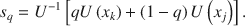
In the second stage of our procedure, we measured probability weighting using several binary choice questions. These questions were constructed on the basis of the subject-specific outcome sequences obtained from the first stage. The subjects chose between a risky prospect
 and a sure outcome
 , where
 and
and
 were two distinct elements of the elicited outcome sequence with
 , and where
 was equal to the certainty equivalent of
 under EU.
This means that
 would be equivalent to
 if the subject with the given utility did not weigh probabilities. Hence by construction, the following logical equivalences held for the given preference relations under RDU.


As we did not allow indifference in our experiment, each choice revealed either the overweighting or underweighting of probability q. Our method made the deviations from EU observable at the aggregate level. For instance, an overweighting of q could be detected when the majority of subjects choose the risky
 , as in logical equivalence (4).
4 The experiment
4.1 Subjects and incentives
The experiment was performed at the ESE-EconLab at Erasmus University in five group sessions. The subjects were 89 Erasmus University students from various academic disciplines (average age 23 years, 40 females). All of the subjects were recruited from a pool of subjects who had never before participated in any economics experiment in our lab, as we sought to avoid subjects who had experienced the TO method. We paid each subject a €5 participation fee. Besides, at the end of each session, we randomly selected two subjects who could play out one of their randomly drawn choices for real. The ten subjects who played for real received €60.70 on average. Over the whole experiment, the average payment per subject was €12.37.
4.2 Procedure
The experiment was run on computers. The subjects were separated by wooden panels to minimize interaction. All of the subjects were provided with paper and pen, and they were instructed that they could take notes if they wished to. Taking notes was not obligatory. Before starting the experiment, the subjects read the general instructions, which included detailed information on the payment procedure, the user interface, and the types of questions they would face. They were allowed to ask questions at any time during the experiment. The experiment consisted of two successive stages without a break in between. Each stage started with a set of instructions and several training questions to familiarize the subjects with the stimuli. These experimental instructions are given in full in Online Appendix 1. Each session took 45 min on average, including the payment phase after the experiment.
4.3 Stimuli
4.3.1 Stage 1: measuring utility
In the first stage of the experiment, a standard sequence of outcomes was elicited by using the TO method. We measured
 , and
, and
 from the following five indifferences, with
 and
and
 :
:

The indifferences were obtained through a bisection method that required seven iterations for each
 . In addition, the last iteration of one randomly chosen
 was repeated at the end of stage 1, to test the reliability of the indifferences. Hence, the subjects answered a total of 36 questions in this part of the experiment. The bisection iteration procedure is described in “Appendix B”. The prospects were presented on the screen, as illustrated in Fig. 3.
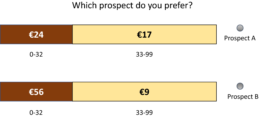
Fig. 3 The choice situation in the TO part
In this part of the experiment, risk was generated by two ten-faced dice, with each die generating one digit of a random number from 00 to 99. In cases where a choice question from this part was implemented for real at the end of the experiment, the outcome of each prospect depended on the result of two dice physically rolled by the subjects.
4.3.2 Stage 2: description versus sampling
Before the start of the experiment’s second part, each subject was randomly assigned to one of the two treatments: description or complete sampling. Here and throughout the next section, we refer to the latter in short as “sampling treatment.” In both treatments, the subjects had to answer seven subject-specific binary choice questions. Each question entailed a choice between a risky prospect
 and the safe prospect
 , as further described in the method section. Note that both
 and
and
 were endogenously determined and varied between subjects.Footnote 4 The values of
 were always rounded to the nearest integer. The seven probabilities used for the investigation of probability weighting were
 . Within each treatment, the orders of the seven questions were counterbalanced. The position of the risky prospect and the safe prospect were also randomized in each question.
The prospects were represented by Ellsberg-type urns, each containing 20 balls with various monetary values attached to them. This way, all the aforementioned probabilities were fractions of 20; i.e., 5% was 1 out of 20, 10% was 2 out of 20, etc. The two treatments differed in terms of how the subjects learned the contents of the urns. In the description treatment, the contents of the urns were explicitly described to the subjects. Figure 4 shows a screenshot of a choice situation for the description treatment.

Fig. 4 A choice situation in the description treatment
Subjects in the sampling treatment were initially given no information about the contents of the urns except the total number of balls. They could only learn about the content of the urns by sampling each ball one-by-one without replacement, and observing the monetary values attached. Figure 5 shows a screenshot of the sampling phase in the sampling treatment. The subjects sampled balls from the urns by clicking “Sample left” or “Sample right” on the screen. Each time they made a selection, the monetary outcome attached to the ball sampled was shown to the subject for 1.5 s before the message disappeared. The subjects could sample the balls at their speed, in whichever order they preferred, and could switch as many times as they wanted, but they could only proceed to the choice stage after sampling all of the balls in both urns.

Fig. 5 Sampling stage in the sampling treatment
Figure 6 shows a screenshot of the choice stage in the sampling treatment. In case a question in this part was implemented for payment at the end, the experimenters set up physical, opaque urns (similar to those that presented on the screen). Each urn was filled with 20 ping-pong balls that were painted either dark blue or light blue, with these colors being associated with the payoffs in question (see Fig. 4). The subjects physically drew a ball from the urn, which determined their payoffs.

Fig. 6 Choice stage in the sampling treatment
The subjects in the description treatment had to answer 21 additional questions following the primary set of 7 questions, to equalize the length of the two treatments. These additional questions concerned another research project.
5 Results
5.1 Reliability and consistency of utility elicitation
In the TO part of the experiment, each subject repeated one choice that she had faced in one of the five indifference elicitations. The repeated choice was randomly selected among the last steps of the iterations. As the subjects were very close to indifference at the last step, this choice was the strongest test of consistency. The subjects made the same choices that they made previously in 70.8% of the cases. Reversal rates up to one third are common in the literature (Stott Reference Stott2006; Wakker et al. Reference Wakker, Erev and Weber1994). Especially if the closeness to indifference is considered, the reversal rates we found were satisfactory. Among the reversed cases, repeated indifferences were higher than the original indifference values in 42.3% of the cases, which did not suggest a systematic pattern (
 , two-sided binomial). Overall, the repeated indifference values did not differ from those of the original elicitations (
 , Wilcoxon sign-rank).
5.2 Utility functions
Table 1 gives descriptive statistics for the elicited outcome sequence.Footnote 5 The parameter
 of the power utility
 was estimated at the individual level by ordinary least squares regression. The average
 was 0.985, which indicated that our estimations fit the data very well.Footnote 6
Table 1 Descriptive statistics for the elicited outcome sequence ( N = 88)

|
Mean |
SD |
Min |
Median |
Max |
|
|---|---|---|---|---|---|
|
|
24.00 |
0.00 |
24.00 |
24.00 |
24.00 |
|
|
60.36 |
23.48 |
30.00 |
58.00 |
118.00 |
|
|
90.36 |
42.58 |
36.00 |
80.00 |
212.00 |
|
|
125.23 |
65.89 |
46.00 |
102.00 |
306.00 |
|
|
164.18 |
91.13 |
52.00 |
134.00 |
400.00 |
|
|
204.14 |
116.25 |
58.00 |
160.00 |
494.00 |
|
|
1.05 |
0.36 |
0.41 |
0.99 |
2.65 |


The summary statistics for the mean and median α are reported in the last row of Table 1. The aggregate data did not deviate from linearity (
 , Wilcoxon sign-rank). Although the mean
 suggested slight convexity, this result was affected by the outliers in our data. Three subjects exhibited extreme convexity with
 , and the skewness/kurtosis test rejected the normality of the distribution of
 s (
s (
 ). The utility estimations did not differ across the two treatments (
 , Wilcoxon rank-sum).Footnote 7
Our data suggested slightly more evidence for concavity than for convexity at the individual level. Considering those subjects whose
 parameters were significantly different from 1 (at a 5% significance level), we find that 30 subjects (15 in the sampling treatment and 15 in the description treatment) exhibited concavity (
 ), and 23 subjects (12 in the sampling treatment and 11 in the description treatment) exhibited convexity (
 ). The proportions of concave and convex utilities did not differ (
 , two-sided binomial). The remaining 35 subjects (40%) did not exhibit significant deviations from linear utility.
5.3 Probability weighting: description versus sampling
5.3.1 Aggregate data
In this section, we report the aggregate choices in the direction of overweighting and underweighting according to logical equivalences (2) and (4) (as presented in the “Method” section). The proportions of overweighting and underweighting of small and large probabilities are given in Figs. 7 and 8, respectively.
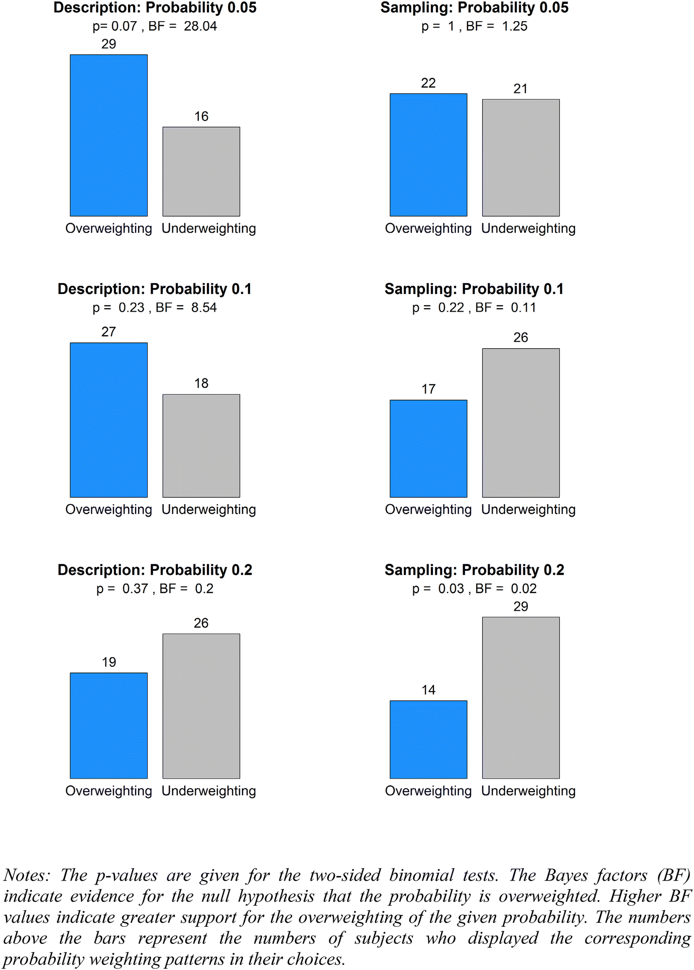
Fig. 7 The weighting of small probabilities

Fig. 8 The weighting of large probabilities
The aggregate choices replicated the common description-experience gap at the extreme probabilities. Overall, the observed gap indicated significantly less overweighting of rare outcomes under the sampling treatment, when assessed on the basis of a repeated-measures logistic regression (
 ).Footnote 8 Based on individual hypothesis tests, the gap was significant at 0.95 (
 ); and was marginally significant at 0.10 and 0.90 (
 , and
, and
 respectively,
 ). The gap at probability 0.05 was not significant (
 ), although the trend suggested reduced overweighting in the sampling treatment. Also, no description-experience gap was apparent in the middle range,
 (
(
 ,
,
 , and
, and
 for
for
 , and 0.80 respectively,
 ).
).
In what follows, we focus on the absolute overweighting and underweighting of probabilities under the two treatments. We first test the deviations from unbiased weighting in either direction by using the two-sided binomial tests for proportions. In addition, to interpret the relative evidence for overweighting and underweighting, we report the Bayes factors for the null hypothesis of overweighting against the alternative hypothesis of underweighting. The Bayes factors indicate the relative evidence for the null hypothesis. For instance, a Bayes factor of 10 indicates that overweighting is 10 times more likely than underweighting for the given probability. Following Jeffreys (Reference Jeffreys1961), we interpret a Bayes factor between 3 and 10 as “some evidence,” a Bayes factor between 10 and 30 as “strong evidence,” and a Bayes factor larger than 30 as “very strong evidence” for the null hypothesis of overweighting. Similarly, Bayes factors of between 0.1 and 0.33, between 0.03 and 0.1, and less than 0.03 are interpreted as “some evidence,” “strong evidence,” and “very strong evidence,” respectively, for the alternative hypothesis of underweighting.Footnote 9
As shown in Fig. 7, for the small probabilities under the description treatment, we found a marginally significant deviation from unbiased weighting at the probability of 0.05 (
 ). Interpreting the results in terms of Bayes factors, we found strong evidence of overweighting 0.05 (
 ), some evidence of overweighting 0.1 (
 ) and some evidence of underweighting 0.2 (
 ). Turning to the small probabilities under the sampling treatment, we found a significantly biased weighting only at the probability of 0.2 (
 ). Interpreting the results in terms of Bayes factors, we found strong evidence of underweighting 0.2 (
 ) and some evidence of underweighting 0.1 (
 ). We found almost no evidence for the underweighting or the overweighting of 0.05 (
 ).
).
For the large probabilities (as shown in Fig. 8) under the description treatment, we found significant biases in the weighting of probabilities 0.8, 0.9, and 0.95 (
 for all). The Bayes factors indicated very strong evidence for underweighting of 0.8, 0.9 and 0.95 (
 for all). Under the sampling treatment, we found significant bias only at 0.8 (
 ). The Bayes factors suggested very strong evidence of underweighting 0.8 (
 ), strong evidence of underweighting 0.9 (
 ), and some evidence of underweighting 0.95 (
 ).
).
Last, we examined the weighting of the moderate 0.5 probability. In the description treatment, 38 out of 45 subjects underweighted 0.5. In the sampling treatment, 36 out of 43 subjects underweighted 0.5. Hence, the deviations from unbiased weighting were highly significant at 0.5 in both treatments (
 for both treatments, two-sided binomial tests). The Bayes factors also indicated very strong evidence in favor of under-weighting at 0.5 (
 for both treatments).
To summarize, our aggregate data replicated the commonly observed inverse S pattern under the description treatment, but provided no evidence for a reversal of the inverse S pattern under the sampling treatment. In particular, we did not observe significant deviations from unbiased weighting at the extreme probabilities 0.05, 0.1, 0.9, or 0.95 in cases where the objective probabilities were learned from sampling without replacement. Notably, no convincing evidence was found for the underweighting of small probabilities 0.05 and 0.1, and more evidence was found for the underweighting than for the overweighting of large probabilities.
5.3.2 Individual data
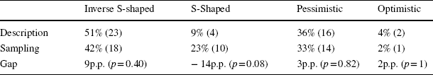
Next, we examined the shapes of the probability weighting functions at the individual level. We classified each subject’s probability weighting function as inverse S-shaped, S-shaped, pessimistic, or optimistic, according to the numbers of over- and under- weightings of three small and three large probabilities, as illustrated in Figs. 7 and 8. These four classes of the probability weighting functions are exhaustive. Specifically, a probability weighting function is inverse S-shaped if it simultaneously overweights at least two out of three small probabilities and underweights at least two out of three large probabilities. The opposite pattern implies an S-shaped probability weighting function. Similarly, a pessimistic probability weighting function underweights at least two small and two large probabilities at the same time, and the opposite pattern implies an optimistic probability weighting function.
Table 2 shows the results of this classification. The probability weighting functions were mainly classified as inverse S-shaped, S-shaped, or pessimistic, and the proportion of optimistic weighting functions was negligible in both treatments. Among the three main types of the probability weighting functions, the majority of cases in the description treatment were inverse S-shaped (
 , one-sided binomial, H0: The proportion of inverse S is
 among inverse S, S, and pessimistic types). Among participants in the sampling treatment, the inverse S-shape was also the most frequently observed, but it did not constitute the majority of cases (
 , one-sided binomial, H0: Proportion of inverse S is
 among the inverse S, S, and pessimistic types).
Table 2 Types of probability weighting functions
|
Inverse S-shaped |
S-Shaped |
Pessimistic |
Optimistic |
|
|---|---|---|---|---|
|
Description |
51% (23) |
9% (4) |
36% (16) |
4% (2) |
|
Sampling |
42% (18) |
23% (10) |
33% (14) |
2% (1) |
|
Gap |
9p.p. (p = 0.40) |
− 14p.p. (p = 0.08) |
3p.p. (p = 0.82) |
2p.p. (p = 1) |
The numbers of probability weighting functions are given in the parentheses. The p-values are results from the (two-sided) Fisher’s exact test
A comparison across the two treatments indicated that the proportion of S-shaped probability weighting functions was higher in the sampling treatment, although the difference was only marginally significant (
 , two-sided Fisher’s exact test). No significant difference appeared between the proportions of inverse S-shaped, pessimistic, and optimistic probability weighting functions across the two treatments.
Overall, our individual-level analysis suggested a reduced but persistent inverse S pattern in the sampling treatment. The results reported above are valid without requiring any parametric assumptions regarding probability weighting or specifications on the stochastic nature of errors. The parametric analysis in the next section supplements our nonparametric results.
5.3.3 Parametric estimations
We performed our parametric analysis of the probability weighting functions by implementing a Bayesian hierarchical estimation procedure. This procedure enables reliable aggregate and individual-level estimations with limited data available per subject. The procedure was recommended by Nilsson et al. (Reference Nilsson, Rieskamp and Wagenmakers2011) and Scheibehenne and Pachur (Reference Scheibehenne and Pachur2015). It has been applied in several other studies for estimating RDU and PT components (Balcombe and Fraser Reference Balcombe and Fraser2015; Kellen et al. Reference Kellen, Pachur and Hertwig2016; Lejarraga et al. Reference Lejarraga, Pachur, Frey and Hertwig2016).
We estimated the Goldstein and Einhorn (Reference Goldstein and Einhorn1987) weighting function, as given by
 .Footnote 10 The parameter
 determines the curvature and captures the sensitivity toward changes in probabilities. In this function,
 indicates an inverse S-shape and likelihood insensitivity, and
 indicates S-shape and likelihood oversensitivity. The parameter
 determines the elevation and captures the degree of pessimism. For
 we have
 . Lower (higher) values of
 indicate less (more) elevation and more (less) pessimism. Following Kruschke (Reference Kruschke2011), we evaluated the credibility of likelihood insensitivity and pessimism based on the ranges of 95% intervals from the posterior distribution of parameters. The details on estimation procedures are given in Online Appendix 5.
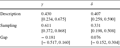
We report the estimated group-level mean parameters and the corresponding 95% credibility intervals in Table 3. Figure 9 shows the estimated probability weighting functions. The estimated parameters indicated credible likelihood insensitivity and pessimism in both treatments, as
 and
and
 both fell on the right side of the 95% credibility intervals. The description-experience gap in terms of likelihood insensitivity and pessimism was not found to be credible, although the difference in likelihood insensitivity was suggestive. Hence, we observed a less pronounced inverse S-shaped weighting function in the sampling treatment, although the elevation was comparable across the two treatments (see the solid curves in Fig. 9).
Table 3 Group level mean parameters
|
|
|
|
|---|---|---|
|
Description |
0.430 [0.234, 0.675] |
0.407 [0.259, 0.590] |
|
Sampling |
0.611 [0.372, 0.868] |
0.331 [0.198, 0.508] |
|
Gap |
− 0.181 [− 0.517, 0.160] |
0.076 [− 0.152, 0.304] |


The estimated parameters are the means of the posterior distributions of the group level means. 95% credibility intervals are given in square brackets
Fig. 9 Probability weighting functions
At the individual level, pessimism (
 ) was credible for all of the subjects in both treatments. Likelihood insensitivity was credible for 51% (23 out of 45) of the subjects in the description treatment and for 29% (13 out of 43) of the subjects in the sampling treatment. Although there was no subject with likelihood oversensitivity (
 ) in the description treatment, 23% (10 out of 43) of the subjects in the sampling treatment exhibited likelihood over-sensitivity, although it was never credible. These results confirmed our previous nonparametric results at the individual level.
6 Discussion
6.1 The two-stage methodology
Our experiment used a two-stage design that separates the measurement of utilities from the measurement of probability weighting. This design circumvented the identification problems that can be caused by potential interactions (collinearities) between utility and probability weighting in simultaneous parametric estimations (Gonzalez and Wu Reference Gonzalez and Wu1999, pp. 152; Scheibehenne and Pachur Reference Scheibehenne and Pachur2015, pp. 403–404; Stott Reference Stott2006, pp. 112; Zeisberger et al. Reference Zeisberger, Vrecko and Langer2012). Our parametric Bayesian hierarchical estimations avoided further averaging biases due to heterogeneous preferences (Nilsson et al. Reference Nilsson, Rieskamp and Wagenmakers2011; Regenwetter and Robinson Reference Regenwetter and Robinson2017). To test the descriptive adequacy of our Bayesian estimations, we compared posterior predictions of the estimated model with the actual data observed (see Online Appendix 5, Figure A5.2). We found that the model was accurate in predicting choices.
One may still be concerned about potential interdependencies between the utility and probability weighting measurements in our two-stage design. Our measurement of probability weighting in the second stage depended on the utilities elicited in the first stage. Thus, any error in the calculation of
 from the first stage could have resulted in a bias in probability weighting measurements. To control for this kind of error propagation, we tested the internal validity of the utility measurements through consistency checks on the elicitations of standard sequences. We used the most stringent test for consistency (see Sect. 5.1 and “Appendix B”), and we found that the rate of consistency was high. In addition, we used parametric fitting in our utility estimations to smooth out the errors (Bleichrodt et al. Reference Bleichrodt, Cillo and Diecidue2010; Etchart-Vincent Reference Etchart-Vincent2004). We observed high goodness-of-fit in our estimations of utility. The direction of rounding in the calculation of
 values did not predict the choices in the second stage (see Online Appendix 7). Our utility estimations indicated slight utility curvature, with some heterogeneity at the individual level. These estimations were close to those reported in previous studies (Abdellaoui Reference Abdellaoui2000; Abdellaoui et al. Reference Abdellaoui, Vossmann and Weber2005; Bleichrodt et al. Reference Bleichrodt, Cillo and Diecidue2010; Qiu and Steiger Reference Qiu and Steiger2010; Schunk and Betsch Reference Schunk and Betsch2006). Our results replicated previous findings on the common inverse S pattern under DFD conditions, and we found the classic description-experience gap, which confirmed the validity of our design.
Another potential concern is the incentive compatibility of the TO method, due to its adaptive nature (with previous choices determine the later stimuli). No previous studies have found this compatibility issue to be a problem in practice (Abdellaoui Reference Abdellaoui2000; Bleichrodt et al. Reference Bleichrodt, Cillo and Diecidue2010; Qiu and Steiger Reference Qiu and Steiger2010; Schunk and Betsch Reference Schunk and Betsch2006; van de Kuilen and Wakker Reference van de Kuilen and Wakker2011). In the terminology used by Bardsley et al. (Reference Bardsley, Cubitt, Loomes, Moffat, Starmer and Sugden2010), this issue might be a concern regarding theoretical incentive compatibility, but not a concern regarding behavioral incentive compatibility (p. 265). Still, as a precautionary measure, we included filler questions in the iteration process of our bisection procedure, intending to make the detection of the adaptive design even more difficult. Our data showed no evidence of strategic choices (see “Appendix B”).
6.2 Beyond the information symmetry
The choice to use a CSP design was motivated by our desire to resolve the information asymmetry between the sampling and the description treatments. The information at the subjects’ disposal was equal in both treatments. However, our complete reliance on sampling experience (without any descriptive information about probabilities) still left room for a discrepancy between the information provided during the sampling stage and the information acquired, or utilized, by the subjects while they made their decisions. This feature of the CSP, which is also a crucial feature of the original paradigm of DFE, distinguishes the CSP from the DFD condition. An exploratory examination of the notes that were taken by the subjects during the experiment suggested the existence of different ways for processing sampling experience (see Online Appendix 8). In particular, although some subjects preferred to take very comprehensive notes of all their sampling observations, others noted only their sampled outcomes without mentioning their frequency or else took no notes at all.Footnote 11 Such heterogeneity in mental processes possibly contributed to the gap observed between the two treatments in our study.Footnote 12 For more discussion on the psychological factors involved in the gap, see Camilleri and Newell (Reference Camilleri and Newell2009).
6.3 Experimental economics research on experience
This study highlights the economic relevance of the DFE research, which to date, has mostly been conducted by researchers in psychology. Our study re-examines the description-experience gap from a behavioral economic perspective. Our DFE experiment relates to the strand of economics literature that investigates the violations of the rationality benchmarks in economic theory. This strand of literature has generally claimed that the standard economic theory performs reasonably well in situations where there is sufficient opportunity for reflection on incentives, deliberation, learning, and experience (Plott Reference Plott, Arrow, Colombatto, Perlaman and Schmidt1996; Binmore Reference Binmore1999). Accordingly, extensive experimental studies have tested the impact of different types of experience on the common anomalies observed in choice experiments. Some examples from this literature include Loomes et al. (Reference Loomes, Starmer and Sugden2003), who documented reductions in discrepancies between willingness to pay and willingness to accept due to repeated market experience. Other examples include Baillon et al. (Reference Baillon, Bleichrodt, Liu and Wakker2016) and Charness et al. (Reference Charness, Karni and Levin2007), who reported reductions in violations of stochastic dominance due to group deliberation and social interactions. van de Kuilen and Wakker (Reference van de Kuilen and Wakker2006) and van de Kuilen (Reference van de Kuilen2009) reported significant convergence to EU maximization under risk in repeated choice settings in cases where immediate feedback was available. Humphrey (Reference Humphrey2006) reported reductions in violations of the independence axiom after observing resolutions of risky lotteries (see Bardsley et al. (Reference Bardsley, Cubitt, Loomes, Moffat, Starmer and Sugden2010) for further discussion of this literature).
Our experimental findings are mostly in line with the previous claims of the literature regarding reductions of irrationalities through experience and deliberation. Both the nonparametric and the parametric analyses indicate that the observed biases in probability weighting were reduced when the objective probabilities were learned more intuitively. Specifically, the sampling experience reduced both the certainty and the possibility effects. We would like to stress that although our study found no pattern of reversed inverse S-shaped probability weighting, this absence of evidence does not necessarily refute any previous assertions in the DFE literature. As clarified in Sect. 2.3, the original claims of underweighting for small probabilities refer to choice propensities, but not to measurements of probability weightings under RDU or PT. What our findings show is that the gap in choice propensities does not translate into a reversal of probabilistic risk attitudes under the RDU framework.
We hope that our study will further contribute to the economics literature by stimulating investigations of the various paradigms of DFE. Further studies involving DFE paradigms could be beneficial for economics research. First, DFD and DFE represent different real-life situations. Although some choice environments provide ample opportunities for learning from experience, others do not. For example, whereas repeated small-scale transactions in the market can allow for trial and error, decision-makers mainly rely on descriptions of the options in making more significant decisions, such as choosing a retirement or health plan. Understanding when and why people exhibit decision biases is ultimately informative for economic policymaking, and for possible implementations of the nudges (Thaler and Sunstein Reference Thaler and Sunstein2008).
Moreover, DFE is a rich experimental environment that can give rise to new theoretical approaches that provide alternatives to the Bayesian approach with EU. For example, some vital aspects of the sampling paradigm, such as memory, adaptive learning, and information search have been previously studied in the DFE literature (Ashby and Rakow Reference Ashby and Rakow2014; Hertwig and Pleskac Reference Hertwig and Pleskac2010; Hills and Hertwig Reference Hills and Hertwig2010; Lejarraga et al. Reference Lejarraga, Hertwig and Gonzalez2012; Kopsacheilis Reference Kopsacheilis2017; Ert and Haruvy Reference Ert and Haruvy2017; Golan and Ert Reference Golan and Ert2015). However, these aspects of sampling are not usually modeled in the traditional decision theories used in economics. To our knowledge, the only decision theory in economics that considers those related aspects is case-based decision theory, as proposed by Gilboa and Schmeidler (Reference Gilboa and Schmeidler1995, Reference Gilboa and Schmeidler2001). Some of the empirical works that investigate this theory include those by Bleichrodt et al. (Reference Bleichrodt, Filko, Kothiyal and Wakker2017), Ossadnik et al. (Reference Ossadnik, Wilmsmann and Niemann2013) and Grosskopf et al. (Reference Grosskopf, Sarin and Watson2015).
7 Conclusion
This study reconsiders the description-experience gap, which to date, has been mostly studied in the literature of psychology. We address the empirical question concerning the gap in risk attitudes induced by the non-linear weighting of probabilities. Our experimental findings support the existence of a description-experience gap, even in cases where objective probabilities from a finite number of sampling observations are available. However, we also find that this gap does not amount to a reversal of the inverse S-shaped probability weighting. In cases where decision-makers are allowed to learn about precise probabilities from experience, their sampling experience tends to reduce the cognitive impairment of likelihood insensitivity.
8 Appendix A: Derivation of the standard sequence of outcomes in TO method
Under RDU, indifferences
 imply
imply
 . A rearrangement of this equation gives
 for all
 . As the right-hand side of the equation is fixed by design, the indifferences result in
 .
.
9 Appendix B: Bisection procedure
The iteration process serves to measure
 and
and
 on the basis of the following indifferences, in which


For each
 , it took five choices to reach the indifference point. Subjects always chose between two prospects:
 and
and
 for
for
 . The procedure was as follows.
1. The initial value of
 was determined as
.
was determined as
.2.
was increased by a given step size when
was chosen over
, and it was similarly decreased when
was chosen over
, as long as
. In case of
was increased to ensure outcome monotonicity.3. The initial step was
, and the step sizes were halved after each choice.4. The indifference point was reached after five choices.
5. The largest possible value of
was
.6. The smallest possible value of
was
. The fourth term on the left-hand side (+16) ensured the monotonicity of outcomes (see point 2).


One concern about the TO method and the bisection iteration process is the method’s incentive compatibility, due to the adaptive design involved. A subject who is fully aware of the adaptive design can strategically drive the value
 upwards by pretending to be extremely risk-averse in response to the bisection questions. In this way, he or she can increase the expected values of prospects in the subsequent questions for the elicitation of
 . To make it more difficult for our subjects to grasp this process fully, we included two filler questions in the iteration process of each
 . These two filler choices were placed after the first and the third choice questions for every
 . In these questions,
 was changed in a direction opposite to that assumed in the changes described in point 2 above. These questions had no further impact on the flow of the procedure.
The filler questions permitted a further test of consistency, as they required preferences that were in line with the previous choices. This kind of preference was required because the preferred option in the previous choice question was made even more attractive in the filler questions. Consistency rates were as high as 97.5% in the first filler question, and 93.3% in the second filler question. The slight decrease of consistency in responses to the second question can possibly be explained by its being closer to the indifference point.
Our data did not suggest any strategic behavior. Although an awareness of the adaptive design from the outset was unlikely, it could be expected that learning during the experiment would lead to increasing distances between
 s. For example, this could lead to larger distances between
 and
and
 than between
 and
and
 . However, the medians of these distances in our data were 26 and 34, respectively, and they did not differ significantly (Wilcoxon sign-rank, p value = 0.54).
Acknowledgements
We thank Peter Wakker, Han Bleichrodt, Aurelien Baillon, Ralph Hertwig, Thorsten Pachur, Orestis Kopsacheilis, and two anonymous reviewers for helpful comments and suggestions on previous versions of the manuscript. The research leading to these results received funding from the Dutch Science Foundation (NWO, Project Number: 406-13-093), Tinbergen Institute, the National Natural Science Foundation of China (Grant Number: 71903006) and the European Research Council (ERC-2013-StG/ERC 336703-RISICO, ERC-336155–COBHAM). Logistic support from the ESE-EconLab at Erasmus University for hosting our experimental sessions is kindly acknowledged.


 Open access