Entry and exit decisions under public and private information: an experiment

Aleksei Chernulich; John Horowitz; Jean Paul Rabanal; Olga Rud; Manizha Sharifova

doi:10.1007/s10683-022-09764-9

Entry and exit decisions under public and private information: an experiment

Published online by Cambridge University Press: 14 March 2025

Olga Rud and

Aleksei Chernulich*: Affiliation:
Center for Behavioral Institutional Design, New York University Abu Dhabi, Abu Dhabi, UAE
John Horowitz*: Affiliation:
Department of Economics, Ball State University, Muncie, USA
Jean Paul Rabanal*: Affiliation:
Department of Economics and Finance, University of Stavanger, Stavanger, Norway
Olga Rud*: Affiliation:
Department of Economics and Finance, University of Stavanger, Stavanger, Norway
Manizha Sharifova*: Affiliation:
Department of Economics, University of the Pacific, Stockton, USA
*: aleksei.chernulich@nyu.edu
jhorowitz@bsu.edu
jeanpaulrab@gmail.com
olga.rud@gmail.com
msharifova@pacific.edu

Article contents

Abstract
Introduction
Environment
Laboratory procedures
Results
Discussion
Funding
Footnotes
References

Rights & Permissions

Abstract

We design an experiment to study how reversible entry decisions are affected by public and private payoff disclosure policies. In our environment, subjects choose between a risky payoff, which evolves according to an autoregressive process, and a constant payoff. The treatments vary the information disclosure rule on the risky payoff, such that in the public information treatment the risky payoff is always observable, while in the private information treatment, the risky payoff is observable only to the participants who enter the market. We find that under private information, market entry is higher, which suggests that subjects engage in exploration and place value on information.

Keywords

Experiment Entry and exit decisions Bandit problems Information provision Forecasting

JEL classification

D84: Expectations • Speculations G11: Portfolio Choice • Investment Decisions C91: Laboratory, Individual Behavior D81: Criteria for Decision-Making under Risk and Uncertainty D83: Search • Learning • Information and Knowledge • Communication • Belief • Unawareness

Type: Original Paper
Information: Experimental Economics , Volume 26 , Issue 2 , April 2023 , pp. 339 - 356

DOI: https://doi.org/10.1007/s10683-022-09764-9 [Opens in a new window]
Creative Commons: This is an Open Access article, distributed under the terms of the Creative Commons Attribution (CC-BY) license (http://creativecommons.org/licenses/by/4.0/), which permits unrestricted re-use, distribution, and reproduction in any medium, provided the original work is properly cited.
Copyright: Copyright © The Author(s) 2022

1 Introduction

A large number of retail transactions occur on centralized online platforms which allow sellers and buyers to seamlessly exchange goods and services. These transactions are easily recorded, often in real time, and offer sellers rich data on consumer preferences. In turn, these data can be used by sellers to forecast future demand with greater precision. Typically, the production decision involves the question of how much to produce, or the intensive margin, and whether to produce, or the extensive margin. The latter is also known as a market entry decision. In this paper, we conduct a laboratory experiment to study how different payoff information affects the market entry decision.

Understanding how subjects respond to information is important for maximizing the profit of market participants, including buyers, sellers, and the designer of the market platform. Profit is often tied to the spell or length of market participation, which is state-dependent. Our experiment allows us to study both components: (i) market entry/exit and (ii) the length of market participation. In the field, studying market entry (or exit) decisions under different information sets may be costly, if not impossible when researchers cannot alter market characteristics. A laboratory experiment can overcome these difficulties by providing complete control over the information available to market participants. In this paper, we present a novel experiment in which the market participants have access to counterfactual information in one environment, but not the other, and in which this decision is reversible. Our primary research question is how the information provided to a subject affects their entry decision. While market transparency for buyers is an actively developing field,Footnote ¹ our experiment allows us to study the impact of transparency on the market’s supply side.

In our environment, market participants can switch between IN and OUT decisions at any time. The payoff to IN follows a stationary AR(1) process, which reflects market conditions. A participant does not have any market power, and therefore takes prices as given. The payoff to OUT is less than the expected payoff to IN. For simplicity, we assume zero transaction costs for switching between IN and OUT and provide subjects with information about the risky payoff generation process. In the private information treatment, which is a typical bandit problem, participants select between a safe arm (OUT), and a risky arm (IN), where the platform provides information in almost real-time. If a participant selects OUT, then the participant will not be able to observe the risky payoff. In order to observe the return to the risky arm, this option must be selected. In the public information treatment, we provide information on the risky payoff regardless of whether the participant is IN or OUT.

To draw predictions for IN and OUT decisions across both treatments, we assume that agents forecast their future revenues under two different rules: (i) rational expectations, and (ii) behavioral expectations which allow for the well-known forecasting biases such as extrapolation and stickiness (Landier et al., Reference Landier, Ma and Thesmar2019). While both rules suggest that IN should be observed more often under public information, we find that subjects select IN more often when information is private. This result suggests that there is a demand for information, and that participants do not exhibit a high degree of risk aversion since they are willing to explore the risky option. These results are also supported by other bandit experiments in the lab (Hoelzemann & Klein, Reference Hoelzemann and Klein2021).Footnote ²

Our experimental design is motivated by the market entry decisions when information flows rapidly. We modify the standard bandit problem found in economics and finance (Bergemann & Välimäki, Reference Bergemann and Välimäki2008) to study reversible entry decisions under different disclosure rules. In a related experiment, Grosskopf et al. (Reference Grosskopf, Erev and Yechiam2006) find that providing counterfactual information in a bandit problem can increase risky behavior. However, this result disappears with more experience, suggesting that subjects become less sensitive to additional information over time. Yechiam and Busemeyer (Reference Yechiam and Busemeyer2006) show that counterfactual information can increase risk taking when the negative outcome is rare and large. Biele et al. (Reference Biele, Erev and Ert2009) employ a Markov process with two states for the risky option, H and L, which are unknown to subjects. They find that players do not learn to become risk averse. In our experiment, we enrich the set of possible outcomes by providing more opportunities for the subjects to familiarize themselves with the payoff realization process due to the nearly continuous environment.Footnote ³

To formulate our predictions, we draw from literature on expectation formation when the predicted variable is exogenous.Footnote ⁴ According to Assenza et al. (Reference Assenza, Bao, Hommes and Domenico2014) and Mokhtarzadeh and Petersen (Reference Mokhtarzadeh and Petersen2020), having access to historical data in forecasting experiments can encourage more adaptive and trend-chasing expectations. Landier et al. (Reference Landier, Ma and Thesmar2019) asked subjects to forecast 40 realizations of a risky asset and found evidence of both sticky (Coibion & Gorodnichenko, Reference Coibion and Gorodnichenko2015; Bouchaud et al., Reference Bouchaud, Kürger, Landier and Thesmar2019), and extrapolative (Bordalo et al., Reference Bordalo, Gennaioli and Shleifer2018) expectations.Footnote ⁵ We simplify the forecasting tasks by focusing on the binary decision of IN or OUT, which indirectly measures market expectations. Our findings complement existing experimental literature on switching behavior (Anufriev et al., Reference Anufriev, Bao and Tuinstra2016, Reference Anufriev, Chernulich and Tuinstra2018 and Anufriev et al., Reference Anufriev, Bao, Sutan and Tuinstra2019). In these experiments, participants were offered an opportunity to switch between investment alternatives. In contrast to our paper, participants in these studies (i) were not informed about the payoff generating process, and (ii) were evaluated only in a public information environment.

2 Environment

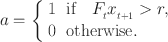
For each $t = {1 \dots, T}$ , a player seeks to maximize profit $π_{t}$ , by choosing between two actions; IN ( $a = 1$ ) and OUT ( $a = 0$ ). Choosing $a = 1$ yields a stochastic payoff $π_{t} = x_{t} + 100$ , in which $x_{t}$ is driven by an autoregressive process of order one AR(1) as specified in Eq. (2), and $ϵ$ follows a standard normal distribution, while OUT, the outside option, yields a constant payoff $r + 100$ , such that

(1)

\begin{matrix} π_{_{t}} = (\begin{matrix} x_{_{t}} + 100 & if a = 1, \\ r + 100 & otherwise, \end{matrix}) \end{matrix}

where

(2)

\begin{matrix} x_{_{t + 1}} = ρ x_{_{t}} + σ \cdot ϵ_{_{t}} . \end{matrix}

The payoff structure that we employ has two important features. First, the payoff for IN, $x_{t}$ , incorporates a risk premium, and therefore $r < E (x_{t})$ . Second, to avoid negative payoffs we add a constant component equal to 100 to both alternatives. We study two environments with different information disclosure rules: public information and private information. In the private information treatment, the subject does not observe the payoff to IN if they choose OUT. In the public information treatment, we provide counterfactual information on the foregone payoff when the subject selects OUT. In both environments, the subject’s decision between IN and OUT at every t is driven by the subject’s beliefs regarding the one period ahead value $x_{_{t + 1}}$ , denoted as $F_{_{t}} x_{_{t + 1}}$ . Consequently,

(3)

\begin{matrix} a = (\begin{matrix} 1 & if F_{_{t}} x_{_{t + 1}} > r, \\ 0 & otherwise . \end{matrix}) \end{matrix}

We allow beliefs $F_{_{t}} x_{_{t + 1}}$ to accommodate a large family of expectations, from Rational Expectations (RE) with $F_{_{t}} x_{_{t + 1}} = E_{_{t}} x_{t + 1} = ρ x_{t}$ , to Sticky and Extrapolative Expectations (SEE) which capture the belief formation for AR(1) processes (Landier et al., Reference Landier, Ma and Thesmar2019). Under SEE, the belief $F_{_{t}} x_{_{t + 1}}$ combines extrapolative expectations, in which subjects overreact to unexpected innovations (Bordalo et al., Reference Bordalo, Gennaioli and Shleifer2018), and sticky expectations (Coibion & Gorodnichenko, Reference Coibion and Gorodnichenko2015, Bouchaud et al., Reference Bouchaud, Kürger, Landier and Thesmar2019), in which subjects demonstrate inertia in updating expectations. We use a nonrecursive specification for the one period ahead forecast, which depends on current and past RE, denoted as $\sum_{k = 0}^{n} E_{_{t - k}} x_{_{t + 1}}$ , as well as the history of x,

(4)

\begin{matrix} F_{_{t}} x_{_{t + 1}} = (1 - λ) \sum_{k = 0}^{n} λ^{k} E_{_{t - k}} x_{_{t + 1}} + γ \sum_{k = 0}^{n} λ^{k} (x_{_{t - k}} - E_{_{t - k - 1}} x_{_{t - k}}) \cdot 1_{_{t - k}}, \end{matrix}

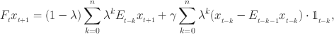
where $λ \in [0, 1]$ is the degree of stickiness, $γ > 0$ captures the importance of extrapolative beliefs, and $1_{t - k}$ takes the value of one when either (i) the environment is public information, and therefore $x_{_{t - k}}$ is always observed, or (ii) the environment is private, and the subject selected IN for $t - k$ . If there is no stickiness to belief updating ( $λ = 0$ ), and no trend extrapolation ( $γ = 0$ ), then the SEE belief is exactly RE, $F_{_{t}} x_{_{t + 1}} = E_{_{t}} x_{_{t + 1}}$ .

Figure 1 shows examples of RE and SEE belief formations using a series of actual x realizations observed by participants in the public and private information treatments with ${ρ, σ, T, r, λ, γ} = {0.85, 12, 160, - 8, 0.21, 0.41}$ . We employ such parameter values for the following reasons. The value of $ρ$ has to be high enough to create an important half-life for innovations $ϵ$ . However, it should not be too close to one in order to avoid a random walk. The value of $σ$ follows the empirical work of Landier et al. (Reference Landier, Ma and Thesmar2019), though we assume a smaller value to mitigate fatigue from facing very volatile series. The value for OUT, r, is obtained from simulations, which create meaningful OUT spells. A smaller value of r incentivizes subjects to stay IN, and therefore limits the ticks in which we can observe players selecting OUT. The last two parameters ( $λ$ and $γ$ ) are the estimates of behavioral expectations parameters reported by Landier et al. (Reference Landier, Ma and Thesmar2019).Footnote ⁶ The solid black line in Fig. 1 shows the value of IN, the RED line represents an agent’s belief under RE, and the blue line represents the belief under SEE. We assume that the simulated player makes a decision according to Eqs. (3) and (4), and does not have information on the risky payoff when selecting OUT. The beliefs of the player evolve upwards after choosing OUT, because the value of IN follows a mean reversion process centered around zero plus the constant of 100.

Fig. 1 Payoff from choosing IN and the evolution of belief under rational expectations (RE) and sticky and extrapolative expectations (SEE). The left panel depicts an example of public information treatment. The right panel depicts an example of private information treatment. The horizontal dashed line represents the value of OUT option and the solid line represents the value of IN option

Hypothesis

Under both behavioral rules, RE and SEE, the frequency of OUT will be lower in the public information treatment than in the private information treatment.

We perform numerical simulations using the observed values of $x_{_{t}}$ (a total of 160-ticks per round) from our experimental sessions to formulate our Hypothesis. We simulate the RE- and SEE-type behavior for all treatments and report the average values of the statistics of interest in Table 1, which include the frequency of staying OUT, the payoff as a fraction of ex-post optimal payoffs, and the switching values of $x_{_{t}}$ .Footnote ⁷ The predictions show that OUT frequency is smaller in the public information treatment. This is due to the mean reversion process of $x_{t}$ and the lower payoff to OUT. This prediction is consistent across the forecasting rules.

We analyze the drivers of behavioral differences across treatments according to the value of x with respect to the payoff to OUT. Conditional on $x < r$ , the simulated player behaves similarly, on average, under both rules, choosing the outside option approximately 70 percent of the time under RE, and opting OUT a bit more frequently under SEE. The main difference arises when $x \geq r$ , where the frequency of IN is smaller in the private information treatment (0.77 under SEE and 0.82 under RE) compared to the public information treatment (0.85 in SEE and 0.88 under RE).

Table 1 Predictions under sticky and extrapolative expectations (SEE) and rational expectations (RE)

	SEE^c		RE
	Public	Private	Public	Private
Frequency OUT^a	0.36	0.39	0.31	0.33
Freq. OUT $\| x < r$ ^b	0.75	0.67	0.69	0.61
Freq. IN $\| x \geq r$	0.85	0.77	0.88	0.82
Payoff as a fraction of ex-post optimal	0.97	0.97	0.97	0.97
Payoff $\| x < r$	0.97	0.96	0.96	0.96
Payoff $\| x \geq r$	0.98	0.98	0.98	0.98
$x + 100$ when switching OUT (all)
Mean	89.45	86.52	86.34	84.11
SD	13.04	14.11	12.44	13.84
$x + 100$ when switching OUT (first)
Mean	91.74	89.19	86.31	87.00
SD	15.62	11.95	13.86	12.88
$x + 100$ when switching IN
Mean	103.07	97.87	101.08	96.13
SD	13.30	20.39	13.30	17.64

^aFrequency of OUT is computed using a tick count of when OUT is selected

^bFrequency of OUT conditional on the realized value of x being below the payoff for OUT

^cSEE (RE) represents the simulation of a player with sticky and extrapolative expectations (rational expectations) using the data generated in the experiment of x for each treatment; 80 series of 160 ticks

In the second section of Table 1, we calculate how the simulated choices perform in terms of the ex-post optimal (maximum) payoff. The predicted behavior is close to optimal under both treatments, and under both forecasting rules. The next section of Table 1 shows the values of x when simulated players switch to OUT and IN. We find that players switch OUT, for both first and all switching decisions, when the value of OUT is below 92, which is in line with our expectations. Regarding the value of x that triggers the switch to IN, we observe it to be slightly higher with public information than with private information. However, the difference is not statistically significant. The predicted comparative statics in the Hypothesis are robust to increasing risk aversion.Footnote ⁸

Alternatively, we may also find that subjects opt IN more often in the private information treatment due to informational demand. Thus, to obtain information on the payoff to x, subjects may (i) delay their decision to switch from IN to OUT, and/or (ii) shorten the OUT spells by re-entering prematurely to gain information about the risky payoff. This alternative hypothesis implies that the value of x that triggers the decision to switch from IN to OUT may be higher in the public information treatment, where players do not gain anything from delaying the decision to switch from IN to OUT. To accurately identify the value of x that triggers switching and separate the effect of exploration, we present summary statistics for the first switching decision, when the information sets are comparable across treatments.

3 Laboratory procedures

The experiments were conducted at the MonLee laboratory in Monash University using oTree software (Chen, Reference Chen, Schonger and Wickens2016). Subjects were recruited online via SONA software and included undergraduate students across all fields. We assigned all participants to one of the two possible treatments: (i) public information, where the information on the foregone payoff is always available, or (ii) private information, where the risky payoff (IN) is unknown when the player opts OUT, and earns a constant payoff.Footnote ⁹

In the instructions, we present the subjects with the underlying AR(1) process and the parameters used. After reading the instructions, subjects answered four control multiple-choice questions.Footnote ¹⁰ If a subject answered a question incorrectly, then the experimenter privately discussed with the participant the relevant section of the instructions.

Each session included two practice rounds, followed by 20 paid rounds. The risky asset payoff was updated every half a second, for 80 s (160 ticks) per round. The value of the risky asset was the same within a session, but all realizations of AR(1) were different between sessions. In total, 83 subjects participated in the experiment. Forty-one subjects participated in the public information treatment, and 42 participated in the private information treatment. Table 2 presents an overview of all laboratory sessions, and an Online Appendix provides dynamic graphs for all experimental sessions.

Table 2 Overview of sessions

	Public	Private
Profit (points per tick)
Mean	101.16	100.11
SD	17.25	17.85
Profit without show-up fee ($)
Mean	10.12	10.01
Show-up fee ($)	10	10
Number of subjects	41	42
Number of sessions	4	4

Subjects were paid in Australian dollars

Figure 2 shows the user interface (UI) in the public information treatment for two different decisions. The left panel of Fig. 2 shows the UI as seen by the subjects when they select IN, and the right panel shows the UI when they select OUT. The UI for the private information treatment is similar to the public information treatment, except that when the player selects OUT, they no longer observe the payoff to IN. The value of IN, $x + 100$ , is depicted as a blue line while the value of OUT appears as a horizontal line at the ordinate value of $r + 100 = 92$ . For each subject, the default initial state is IN. If the current strategy is IN, subjects can switch OUT by clicking the “GET OUT" button located at the bottom of the interface, and if the current strategy is OUT, subjects can switch IN by clicking the “GET IN" button also located at the bottom of the interface. Players can switch between IN and OUT each tick, which lasts half a second, for $T - 1$ ticks. The green shaded area represents the accumulated payoffs. When a subject selects OUT, the payoffs accumulate at the constant rate of 92 points per tick (see right panel of Fig. 2).

Fig. 2 User interface in the public information treatment: (i) left panel shows the payoff (in green) for staying IN up to tick 30, and (ii) right panel shows the payoff (in green) if a subjected switched OUT at tick 30. (Color figure online)

After each round ends, we show subjects the points accrued in that round, and the cumulative points earned from all non-practice rounds. The experimental sessions lasted about 50 minutes. At the end of the session, the points earned across all rounds were added and converted to cash at the exchange rate of $.003125 per 100 points. Excluding the show-up fee of $10, subjects received on average $10.12 in the public information treatment and $10.01 in the private information treatment (see Table 2). The two treatments have similar payoffs, which is consistent with our predictions, due to the mean reversion process that governs the evolution of the value of IN. Despite the similarities in average values, we observe important differences in behavior when the value of x goes below the outside option payoff.

4 Results

We begin our discussion of results with Fig. 3, which shows an example of a round from each treatment.Footnote ¹¹

Fig. 3 Evolution of x (blue) and fraction of players (red) in a session selecting IN for the public (left) and private (right) treatments. The black dotted line is the outside option payoff. (Color figure online)

The left panel of Fig. 3 presents the results for the public information treatment, while the right panel presents the results for the private information treatment. The blue line depicts the value of $x + 100$ , measured against the left y-axis, while the red line shows the fraction of subjects who choose IN, measured against the right y-axis, at time t. The black line is the outside option payoff. We observe that subjects actively move IN and OUT of the market throughout the round. When the value of IN is high, more players select the risky option (such that the fraction of subject IN approaches 1), and when the value of IN is low, more players choose the outside option.

Figure 4 provides a summary of the observed frequency of OUT spells and the duration of the median OUT spell for both treatments. The black bar shows the results for the public information treatment, while the grey bar shows the results for the private information treatment. According to the left panel, subjects stay OUT more frequently in the public information treatment. Similarly, the median OUT spell duration is also longer in the public information treatment.

Fig. 4 Summary of results (pooled data): (i) frequency of OUT (left panel), and (ii) median spell OUT (right panel). Under RE, the frequency of OUT is 0.31 and 0.33 for public and private treatments, respectively, while the median OUT spell is 2 and 4 for public and private treatments, respectively

Next, we study the cumulative distribution function (CDF) in Fig. 5 which shows the fraction of ticks when subjects select OUT. The CDF for the public information treatment first order stochastically dominates the distribution for the private information treatment, which is consistent with the larger mean frequency of OUT in Fig. 4.

Fig. 5 CDF of the fraction of OUT choices in the private versus public information treatments (pooled data)

To study subject behavior over time, we present summary statistics in Table 3 using data from (i) all rounds, and (ii) rounds 11 through 20. We find that experience does not affect subject behavior, with both data samples showing similar outcomes for each treatment. To better understand the observed behavior, we compute the frequency of IN conditional on the value of x being equal to or greater than the outside option payoff (IN $∣$ $x \geq r$ ), and the frequency of OUT conditional on the value of x being below the outside option payoff (OUT $∣$ $x < r$ ). When IN is more profitable, subjects select IN 72 percent of the time in the public information treatment and 79 percent of the time in the private information treatment. When OUT is more profitable, subjects play OUT 60 percent of the time in the public information treatment and 41 percent of the time in the private information treatment. The second section of Table 3 calculates the relative payoff as a fraction of the ex-post optimal payoff. Overall, players perform slightly worse than the predicted payoff of 0.97 under both forecasting rules.

Table 3 Summary statistics

	All rounds		Rounds 11–20
	Public	Private	Public	Private
Frequency OUT ^a	0.38	0.28	0.40	0.29
Obs.	128,000	131,200	64,000	64,000
Freq. OUT $\| x < r$ ^b	0.60	0.41	0.61	0.43
Freq. IN $\| x \geq r$	0.72	0.79	0.71	0.79
Payoff as a fraction of ex-post optimal	0.96	0.95	0.96	0.95
Payoff $\| x < r$	0.95	0.92	0.95	0.92
Payoff $\| x \geq r$	0.96	0.97	0.96	0.97
$x + 100$ when switching OUT (all)
Mean	89.37	85.43	88.77	84.66
SD	15.97	15.99	15.27	16.03
$x + 100$ when switching OUT (first)
Mean	88.77	85.27	87.50	85.08
SD	17.81	15.41	18.08	15.64
$x + 100$ when switching IN
Mean	104.17	95.62	103.67	94.36
SD	17.83	20.41	17.33	19.75

^aFrequency of OUT is computed using a tick count of when the OUT strategy is observed

^bFrequency of OUT conditional on the realized value of x being below the risky-free payoff

In the third section of Table 3, we compute the mean value of x that triggers players to switch from IN to OUT. For the public information treatment, the value is close to the outside option payoff of 92. For the private information treatment, players wait until $x + 100$ drops to 85 to switch from IN to OUT. The observed value of x is sightly above the RE prediction of 86 in the public information treatment, and close to the RE prediction of 84 in the private information treatment.Footnote ¹²

The last section of Table 3 presents the value of $x + 100$ that triggers the decision to select IN. In the public information treatment, subjects require approximately 104 points to select IN again. In the private information treatment, where subjects do not observe the value of IN while OUT, subject require a lower payoff of 96 to re-enter the market. A lower trigger value in the private information treatment is consistent with the shorter OUT duration in the private information treatment, where subjects switch sooner due to the lack of information.

Result 1

Subjects select OUT more often in the public information treatment.

According to the linear probability model presented in Table 4, subjects are more likely to select OUT in the public information treatment, contrary to the hypothesis.Footnote ¹³ The dependent variable takes the value of one when the subject selects OUT, and zero when the subject selects IN for all specifications except (III), where the definition is reversed. Further, in specifications (III) and (IV), the probability is conditional on the value of x. The dummy variable Private is the treatment effect, which equals one if the subject is in the private information treatment and zero otherwise. The dummy variable Round is the trend effect, which controls for learning. We find that, on average, the frequency of OUT in the private information treatment is 10 percentage points lower than in public information treatment.

Table 4 Linear probability model

	(I)	(II)	(III)	(IV)
	OUT	OUT	IN $\| x \geq r$	OUT $\| x < r$
Intercept	0.384***	0.359***	0.724***	0.597***
Intercept	(0.009)	(0.011)	(0.012)	(0.009)
Private	− 0.103***	− 0.103***	0.064***	− 0.182***
Private	(0.016)	(0.016)	(0.018)	(0.018)
Round	–	− 0.002***	–	–
Round	–	(0.02)	–	–
$R^{2}$	0.01	0.01	0.01	0.03
N	259 200	259,200	170,305	88,895

The Intercept captures the public information treatment. Standard errors are in parenthesis, clustered at the subject level and computed via bootstrapping. ***p ≤ 0.01, **p ≤ 0.05, *p ≤ 0.1

Specification (III), which restricts the sample to when the risky option outperforms the outside option, suggests that players in the private information treatment stay IN more often than players in the public information treatment. The largest difference in behavior is observed in specification (IV), which restricts the sample to observations where the risky option under-performs the outside option. In this subsample, the frequency of OUT in the private information treatment is 18 percentage points lower. If information had no value, then we would not observe OUT more often in the private information treatment (see Table 1). Thus, specification (IV) suggests that subjects in the private information treatment value information because they are willing to stay IN. To confirm that these results are robust, Table 9 in Appendix A presents the linear regression results for rounds in which the value of IN is below 80 for at least 40 ticks. We conclude that the treatment differences are robust to when players are in markets with a low rate of return.

Result 2

Duration of an OUT spell, or uninterrupted time spent OUT without switching, is longer in the public information treatment.

To analyze the duration of an OUT spell, we use a Weibull survival function,

\begin{matrix} S (t; p, z_{j} β) = exp (- λ_{_{j}} t_{_{j}}^{p}), \end{matrix}

where t is the number of ticks that a player chooses OUT, p is the shape parameter and $λ_{_{j}} = exp (z_{j} β)$ , which includes the regressors ( $z_{_{j}}$ ) and the coefficient ( $β$ ). The hazard rate is computed as

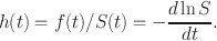
\begin{matrix} h (t) = f (t) / S (t) = - \frac{d ln S}{dt} . \end{matrix}

The estimated parameters of the hazard function are presented in Table 5, and the survival function S(t) is shown in Fig. 6. The standard errors in the parametric estimation are clustered at the subject level. We find that $p < 1$ , which indicates that h(t) is a decreasing function. Note that in each round, we observe multiple OUT spells.

The survival function confirms that subjects in the public information treatment stay out longer (solid black line) than in the private information treatment (dashed green line). We estimate the survival function using the parameters from Table 5 and find that the coefficient for Private is 0.36, and the hazard rate is $1.43 (= exp (0.36))$ in the private information treatment relative to public information treatment. Shorter OUT spells in the private information treatment confirm that information has value– subjects choose IN to determine and evaluate the payoff of x relative to the outside option OUT. In the public information treatment, subjects know the value of x and can evaluate the relative payoff without switching prematurely. Hence, subjects are willing to opt OUT of the risky option more often in the public information treatment because they do not lose access to information.

Fig. 6 Weibull survival function: $O U T \to$ IN

Table 5 Hazard function

Intercept	− 1.89***
Intercept	(0.06)
Private	0.36***
Private	(0.14)
$log (p)$	− 0.16***
$log (p)$	(0.03)
$ψ$	6.96
N	86,169

To compute the hazard ratios, we use an $exp$ function on relevant coefficients. ***p ≤ 0.01, **p ≤ 0.05, *p ≤ 0.1

Result 3

Subjects select OUT faster in the public information treatment.

To determine when subjects switch from IN to OUT, we use a Tobit regression. Since we are interested in a point estimate rather than the duration of an event, a Tobit regression can provide a more precise estimate than a Weibull survival analysis. The decision to switch OUT is dependent on observing a sufficiently low value of x. Therefore, we address possible censoring issues by using the Tobit regression.

Table 6 summarizes the results of the Tobit regressions for the value of x when subjects switch from $I N \to$ OUT in specifications (I) and (II). Specification (I) analyzes all IN/OUT decisions, while specification (II) focuses only on the first IN/OUT switch. In the public information treatment, subjects switch when $x + 100$ is around 90. In the private information treatment, subjects switch when x is about 3.94 points lower. In other words, subjects in the public information treatment do not wait as long to exit (select OUT). This difference can be explained by the fact that the value of x is always available in the public information treatment, and therefore, the payoff to each strategy is clear. In the private information treatment selecting OUT reduces the information available. Thus, waiting to select OUT suggests that subjects demand information on the relative payoff.

Table 6 Switching value of $x + 100$

	(I)	(II)	(III)
	$x + 100$ : $I N \to$ OUT	$x + 100$ : $I N \to$ OUT	$x + 100$ : $O U T \to$ IN
	All	First	All
Intercept	89.37***	88.77***	104.91***
Intercept	(0.55)	(1.11)	(0.64)
Private	− 3.94***	− 3.49**	− 8.51***
Private	(0.79)	(1.36)	(0.78)
Pseudo $R^{2}$	0.002	0.001	.003
N	14,343	1606	13,820

All specifications are estimated using a Tobit regression. The intercept indicates the value of $x + 100$ in the public information treatment. Standard errors are in parenthesis, clustered at the subject level and computed via bootstrapping. ***p ≤ 0.1, **p ≤ 0.5, *p ≤ 0.1

Result 4

Subjects wait longer to select IN in the public information treatment.

Specification (III) in Table 6 shows the value of x when subjects switch from OUT $\to$ IN. We find that in the public information treatment subjects wait longer to re-enter, and that when subjects switch, the value of x is close to 105. In the private information treatment, the subject is uninformed about x and therefore its particular value is not as meaningful. In this environment, subjects switch IN to learn the payoff to x, while in the public information environment subjects react to the value of x. The shorter duration of the OUT spell is consistent with a lower value of x observed in the OUT $\to$ IN decision in the private information treatment.

5 Discussion

In this paper, we study market entry decisions, where the payoff to entry is governed by a stationary AR(1) process, while market exit guarantees a constant payoff, under alternative information disclosure policies. In the public information treatment, we provide information on forgone payoffs to market entry, while in the private information treatment the subjects learn about market payoffs only if they enter the market. We introduce a nearly continuous environment where the risky payoff is updated every 0.5 s,Footnote ¹⁴ and omit point forecast elicitation.

Our results show that market entry is higher by about 10 percentage points when we omit information about foregone payoffs. While we observe strong treatment differences, the payoffs under both public and private information treatments are quite similar. The small difference may be due to the mean reversion process which governs the evolution of the risky payoff.Footnote ¹⁵ It would be interesting to study whether a process other than mean reversion leads to a different conclusion. However, we hypothesize that the behavior will be consistent due to demand for information in the private information treatment, but with larger payoff differences.

The analysis presented in this paper is motivated by the modern online retail platforms. In these markets, information flows continuously, and profit of market participants might depend on the time spent on the platform. We show that information about the state of the market is important for participation, and that the extent of information disclosure has consequences for market entry, and exit decisions. We also believe that our results are applicable to other settings. For example, managers can potentially increase participation rates in investment ventures by selectively disclosing payoff information to clients. Furthermore, one can extend our design to analyze how the decisions of others affect individual entry decisions. In a related bandit experiment, Hanaki et al. (Reference Hanaki, Kirman and Pezanis-Christou2018) show that providing information about the decisions of others can help maximize profit, while in an exponential bandit problem, Hoelzemann and Klein (Reference Hoelzemann and Klein2021) find an increase in free-riding on the information produced by partners. Alternatively, one can also study how almost continuous-time affects the evolution of prices in learning-to-forecast experiments (Hommes, Reference Hommes, Sonnemans, Tuinstra and Van de Velden2005, and recently Arifovic and Petersen, Reference Arifovic and Petersen2017 and Kopányi, Reference Kopányi, Rabanal, Rud and Tuinstra2019). We leave these ideas for future research.

Acknowledgements

We are grateful for the insightful discussions and comments received from the Editors Ragan Petrie and Roberto Weber, two anonymous referees, Dan Friedman, John Duffy, Tibor Neugebauer, Luba Petersen, Nick Feltovich, Sébastien Pouget, Peter Bossaerts, Philip Drummond, Diego Aycinena, Pedro Romero, Robert Durand as well as from participants in numerous seminars and workshops. This project was approved by the human subjects committee at Monash University. Aleksei Chernulich is grateful for financial support from Tamkeen under the NYUAD Research Institute award for Project CG005.

Funding

Open access funding provided by University Of Stavanger.

Footnotes

Supplementary Information The online version contains supplementary material available at https://doi.org/10.1007/s10683-022-09764-9.

The replication material for the study is available at https://doi.org/10.17605/OSF.IO/ET3KF.

¹ See Kaya and Liu (Reference Kaya and Liu2015), Fuchs et al. (Reference Fuchs, Öry and Skrzypacz2016), Bergemann and Hörner (Reference Bergemann and Hörner2018).

² In multi-armed bandit problems, Hudja and Woods (Reference Hudja and Woods2021) observe decreasing switching rates over time.

³ The payoff realization process occurs twice per second, and helps capture the instantaneous feedback of modern retail markets.

⁴ See Schmalensee (Reference Schmalensee1976), Dwyer et al. (Reference Dwyer, Williams, Battalio and Mason1993), Hey (Reference Hey1994), Kelley and Friedman (Reference Kelley and Friedman2002), Glaser et al. (Reference Glaser, Langer, Reynders and Weber2007) and Beshears (Reference Beshears, Choi, Fuster, Laibson and Madrian2013).

⁵ For empirical evidence using expectations survey data, please refer to Gene and Sharpe (Reference Amromin and Sharpe2013); Gennaioli et al. (Reference Gennaioli, Ma and Shleifer2016) and Wen (Reference Wen2018). For an overview of the interactions of individual forecasting rules, and the aggregate macro behavior they co-create, refer to Assenza et al. (Reference Assenza, Bao, Hommes and Domenico2014).

⁶ Landier et al. (Reference Landier, Ma and Thesmar2019) results are robust to a family of values of ρ ∈ { 0 , 0.2 , 0.4 , 0.8 , 1 } , and a value of σ = 20 . Given our tick size, the equivalent standard deviation is 14.142 = 20 / 2 for our design.

⁷ Information on OUT spells for the simulated behavior is available in Appendix C.

⁸ Risk neutrality does a good job in explaining the behavior in dynamic environments. For example, see (Magnani & Munro , Reference Magnani and Munro2020) who also state their predictions under risk neutrality in a dynamic experiment. For robustness, we allow for risk aversion and assume a power utility, u α where α ∈ { 0.3 , 0.5 } .

⁹ The instructions for the public information treatment are in the online repository. The key differences in wording across instructions are: When you switch to OUT, you will stop observing the variable payoff of IN for the private information treatment, and When you switch to OUT, you will still observe the variable payoff of IN for the public information treatment.

¹⁰ We asked subjects to answer the following: (i) what is the average payoff of IN?, (ii) if you select OUT, then you accumulate points according to (100, x, 92, 0), (iii) if you switch from OUT to IN, can you switch again and go OUT? (iv) Does the current value of x affect the value of x in the next period?

¹¹ Appendix D has the complete time-series observations for all experimental sessions.

¹² Appendix C presents data on the duration of OUT spells for the 10th, 25th, 50th, 75th, and 90th percentiles, where the top percentiles indicate the shortest duration. While there is no difference in the duration of an OUT spell at the 10th and 25th percentiles between the two treatments, the median duration of an OUT spell is two ticks greater in the public information treatment than the private information treatment.

¹³ In the working paper, we also control for the risk attitudes of participants following the protocol of Crosetto and Filippin (Reference Crosetto and Filippin2013). However, all risk data (except for one session) was lost when one of authors transferred files following a change in employment. In Appendix A, Table 7, we present the main regression from the working paper, which controls for risk. The treatment effect has a similar coefficient: the frequency of OUT in the private information treatment is 10 percentage points lower than in public information treatment. In Table 8, we present the analysis of the hazard rate for switching from OUT to IN, and find that the results do not substantively change if this measure is included. This is not surprising since it is hard to explain the dynamic choices observed in our experiment with standard static risk elicitation tasks.

¹⁴ For other nearly continuous environments, refer to Cason et al. (Reference Cason, Friedman and Hopkins2014), Friedman et al. (Reference Friedman, Huck, Oprea and Weidenholzer2015), and Bosch-Rosa (Reference Bosch-Rosa2018).

¹⁵ In our sessions, the mean payoff to OUT is 0.67 standard deviations below the mean payoff to IN.

Springer Nature remains neutral with regard to jurisdictional claims in published maps and institutional affiliations.

References

Amromin, G., & Sharpe, S. A. (2013). From the horse’s mouth: Economic conditions and investor expectations of risk and return. Management Science, 60(4), 845–866. 10.1287/mnsc.2013.1806CrossRef Google Scholar

Anufriev, M., Chernulich, A., & Tuinstra, J. (2018). A laboratory experiment on the heuristic switching model. Journal of Economic Dynamics and Control, 91, 21–42. 10.1016/j.jedc.2018.04.004CrossRef Google Scholar

Anufriev, M., Bao, T., & Tuinstra, J. (2016). Microfoundations for switching behavior in heterogeneous agent models: An experiment. Journal of Economic Behavior & Organization, 129, 74–99. 10.1016/j.jebo.2016.06.002CrossRef Google Scholar

Anufriev, M., Bao, T., Sutan, A., & Tuinstra, J. (2019). Fee structure and mutual fund choice: An experiment. Journal of Economic Behavior & Organization, 158, 449–474. 10.1016/j.jebo.2018.12.013CrossRef Google Scholar

Arifovic, J., & Petersen, L. (2017). Stabilizing expectations at the zero lower bound: Experimental evidence. Journal of Economic Dynamics and Control, 82, 21–43. 10.1016/j.jedc.2017.04.005CrossRef Google Scholar

Assenza, T., Bao, T., Hommes, C., & Domenico, M. et al., (2014). Experiments on expectations in macroeconomics and finance. Experiments in Macroeconomics, 17, 11–70. 10.1108/S0193-230620140000017002CrossRef Google Scholar

Bergemann, D., & Hörner, J. (2018). Should first-price auctions be transparent?. American Economic Journal: Microeconomics, 10(3), 177–218.Google Scholar

Bergemann, D., & Välimäki, J. (2008). Bandit problems. The New Palgrave Dictionary of Economics, 1–8, 336–340.Google Scholar

Beshears, J., Choi, J. J., Fuster, A., Laibson, D., & Madrian, B. C. (2013). What goes up must come down? Experimental evidence on intuitive forecasting. American Economic Review, 103(3), 570–74 10.1257/aer.103.3.570CrossRef Google Scholar PubMed

Biele, G., Erev, I., & Ert, E. (2009). Learning, risk attitude and hot stoves in restless bandit problems. Journal of Mathematical Psychology, 53(3), 155–167. 10.1016/j.jmp.2008.05.006CrossRef Google Scholar

Bordalo, P., Gennaioli, N., & Shleifer, A. (2018). Diagnostic expectations and credit cycles. The Journal of Finance, 73(1), 199–227. 10.1111/jofi.12586CrossRef Google Scholar

Bosch-Rosa, C. (2018). That’s how we roll: An experiment on rollover risk. Journal of Economic Behavior & Organization, 145, 495–510. 10.1016/j.jebo.2017.11.005CrossRef Google Scholar

Bouchaud, J-P, Kürger, P., Landier, A., & Thesmar, D. (2019). Sticky Expectations and the Profitability Anomaly. The Journal of Finance, 74(2), 639–674. 10.1111/jofi.12734CrossRef Google Scholar

Cason, T. N., Friedman, D., & Hopkins, E. (2014). Cycles and instability in a rock-paper-scissors population game: A continuous time experiment. Review of Economic Studies, 81(1), 112–136. 10.1093/restud/rdt023CrossRef Google Scholar

Chen, D. L., Schonger, M., & Wickens, C. (2016). oTree-An open-source platform for laboratory, online, and field experiments. Journal of Behavioral and Experimental Finance, 9, 88–97. 10.1016/j.jbef.2015.12.001CrossRef Google Scholar

Coibion, O., & Gorodnichenko, Y. (2015). Information rigidity and the expectations formation process: A simple framework and new facts. American Economic Review, 105(8), 2644–78 10.1257/aer.20110306CrossRef Google Scholar

Crosetto, P., & Filippin, A. (2013). The “bomb” risk elicitation task. Journal of Risk and Uncertainty, 47(1), 31–65. 10.1007/s11166-013-9170-zCrossRef Google Scholar

Dwyer, G. P., Williams, A. W., Battalio, R. C., & Mason, T. I. (1993). Tests of rational expectations in a stark setting. The Economic Journal, 103(418), 586–601. 10.2307/2234533CrossRef Google Scholar

Friedman, D., Huck, S., Oprea, R., & Weidenholzer, S. (2015). From imitation to collusion: Long-run learning in a low-information environment. Journal of Economic Theory, 155, 185–205. 10.1016/j.jet.2014.10.006CrossRef Google Scholar

Fuchs, W., Öry, A., & Skrzypacz, A. (2016). Transparency and distressed sales under asymmetric information. Theoretical Economics, 11(3), 1103–1144. 10.3982/TE2237CrossRef Google Scholar

Gennaioli, N., Ma, Y., & Shleifer, A. (2016). Expectations and investment. NBER Macroeconomics Annual, 30(1), 379–431. 10.1086/685965CrossRef Google Scholar

Glaser, M., Langer, T., Reynders, J., & Weber, M. (2007). Framing effects in stock market forecasts: The difference between asking for prices and asking for returns. Review of Finance, 11(2), 325–357. 10.1093/rof/rfm008CrossRef Google Scholar

Grosskopf, B., Erev, I., & Yechiam, E. (2006). Foregone with the wind: Indirect payoff information and its implications for choice. International Journal of Game Theory, 34(2), 285–302. 10.1007/s00182-006-0015-8CrossRef Google Scholar

Hanaki, N., Kirman, A., & Pezanis-Christou, P. (2018). Observational and reinforcement pattern-learning: An exploratory study. European Economic Review, 104, 1–21. 10.1016/j.euroecorev.2018.01.009CrossRef Google Scholar

Hey, J. D. (1994). Expectations formation: Rational or adaptive or ...?. Journal of Economic Behavior & Organization, 25(3), 329–349. 10.1016/0167-2681(94)90104-XCrossRef Google Scholar

Hoelzemann, J., & Klein, N. (2021). Bandits in the Lab. Quantitative Economics, 12(3), 1021–1051. 10.3982/QE1389CrossRef Google Scholar

Hommes, C., Sonnemans, J., Tuinstra, J., & Van de Velden, H. (2005). Coordination of expectations in asset pricing experiments. The Review of Financial Studies, 18(3), 955–980. 10.1093/rfs/hhi003CrossRef Google Scholar

Hudja, S., & Woods, D. (2021). An exploratory analysis of the multi-armed bandit problem. Available at SSRN 3942930.CrossRef Google Scholar

Kaya, A., & Liu, Q. (2015). Transparency and price formation. Theoretical Economics, 10(2), 341–383. 10.3982/TE1566CrossRef Google Scholar

Kelley, H., & Friedman, D. (2002). Learning to forecast price. Economic Inquiry, 40(4), 556–573. 10.1093/ei/40.4.556CrossRef Google Scholar

Kopányi, D., Rabanal, J. P., Rud, O. A., & Tuinstra, J. (2019). Can competition between forecasters stabilize asset prices in learning to forecast experiments?. Journal of Economic Dynamics and Control, 109, 103770 10.1016/j.jedc.2019.103770CrossRef Google Scholar

Landier, A., Ma, Y., & Thesmar, D. (2019). Biases in expectations: Experimental evidence.Google Scholar

Magnani, J., & Munro, D. (2020). Dynamic runs and circuit breakers: An experiment. Experimental Economics, 23(1), 127–153. 10.1007/s10683-019-09602-5CrossRef Google Scholar

Mokhtarzadeh, F., & Petersen, L. (2020). Coordinating expectations through central bank projections. Experimental Economics, 24, 1–36.Google Scholar PubMed

Schmalensee, R. (1976). An experimental study of expectation formation. Econometrica, 44(1), 17–41. 10.2307/1911378CrossRef Google Scholar

Wen, Q. (2018). Asset growth and stock market returns: A time-series analysis. Review of Finance, 23(3), 599–628. 10.1093/rof/rfy018CrossRef Google Scholar

Yechiam, E., & Busemeyer, J. R. (2006). The effect of foregone payoffs on underweighting small probability events. Journal of Behavioral Decision Making, 19(1), 1–16. 10.1002/bdm.509CrossRef Google Scholar