The effects of conflict budget on the intensity of conflict: an experimental investigation

Kyung Hwan Baik; Subhasish M. Chowdhury; Abhijit Ramalingam

doi:10.1007/s10683-019-09615-0

The effects of conflict budget on the intensity of conflict: an experimental investigation

Published online by Cambridge University Press: 14 March 2025

Kyung Hwan Baik ,

Subhasish M. Chowdhury and

Abhijit Ramalingam

Show author details

Kyung Hwan Baik: Affiliation:
Department of Economics, Sungkyunkwan University, 03063 Seoul, South Korea
Subhasish M. Chowdhury*: Affiliation:
Department of Economics, University of Bath, BA2 7AY Bath, UK
Abhijit Ramalingam: Affiliation:
Department of Economics, Appalachian State University, 28608 Boone, NC, USA
*: s.m.chowdhury@bath.ac.uk

Article contents

Abstract
Introduction
Theoretical benchmark
Experimental procedure and hypothesis
Results
Discussion
Footnotes
References

Rights & Permissions

Abstract

We experimentally investigate the effects of conflict budget on conflict intensity. We run a between-subjects Tullock contest in which we vary the contest budget from Low to Medium to High, while keeping the risk-neutral Nash equilibrium bid the same. We find a non-monotonic relationship: bids increase when the budget increases from Low to Medium, but decrease when the budget further increases from Medium to High. This can happen for players with concave utility, if a high budget has a wealth effect that reduces the marginal utility of winning resulting in lower bids. To test this, we run a Wealth treatment in which the budget remains the Medium, but contestants receive a fixed payment (as wealth) independent of the contest outcome. The bids in the Wealth treatment are lower than the Medium treatment, but are not different from the High treatment, supporting the hypothesis of a wealth effect. We then support this empirical observation by a theoretical model with risk-aversion.

Keywords

Conflict Experiment Budget constraint Wealth effect

JEL classification

D74: Conflict • Conflict Resolution • Alliances • Revolutions C91: Laboratory, Individual Behavior D72: Political Processes: Rent-Seeking, Lobbying, Elections, Legislatures, and Voting Behavior C72: Noncooperative Games

Type: Original Paper
Information: Experimental Economics , Volume 23 , Issue 1 , March 2020 , pp. 240 - 258

DOI: https://doi.org/10.1007/s10683-019-09615-0 [Opens in a new window]
Creative Commons: This is an Open Access article, distributed under the terms of the Creative Commons Attribution (CC-BY) license (http://creativecommons.org/licenses/by/4.0/), which permits unrestricted re-use, distribution, and reproduction in any medium, provided the original work is properly cited.
Copyright: Copyright © The Author(s) 2019

1 Introduction

Conflicts, in which individuals or groups “try to hamper, disable, or destroy rivals” (Hirshleifer Reference Hirshleifer, Hartley and Sandler1995), are ubiquitous. Some examples are warfare, civil disputes, ethnic clashes, terrorism and defense, gang fights, litigation, and rent-seeking. Agents make sunk investments of resources in the conflict in order to win a reward such as winning a war, gaining prestige, or taking revenge. The availability of such resources, i.e., the conflict budget, is one of the most important elements that determine the intensity of conflicts, i.e., the amount of resources invested. In this study we experimentally investigate this relationship between conflict budget and the intensity of conflict.

One popular way to study conflict is to employ the models of contest theory, in which agents place sunk bids that affect the probability of winning a reward (Konrad Reference Konrad2009). In a basic model, conflict intensity is not affected by changes in the available budget, as long as it is above the equilibrium bid. However, it is observed in the laboratory that the budget can affect behavior in a variety of non-conflict experiments where the budget is not expected to play a role. Examples include social dilemmas (Clark Reference Clark2002), risky choices (Bosch-Domènech and Silvestre Reference Bosch-Domènech, Silvestre, Schultz and Vind2006), cooperation and punishment (Kocher et al. Reference Kocher, Martinsson and Visser2008), and altruism (Chowdhury and Jeon Reference Chowdhury and Jeon2014). The effect of budget in the conflict or contest literature, however, is unexplored. We are not aware of any experiment that seeks to answer this specific question. We fill this gap in the literature.

We run a contest experiment in which we vary the budget from Low to Medium to High in different treatments, but keep the risk-neutral Nash equilibrium bid the same. Conflict intensity first increases when conflict budget is increased from Low to Medium, but then it decreases when the conflict budget is increased further from Medium to High. We then run a Wealth treatment in which the budget remains the Medium, but agents receive an additional fixed payment (wealth) independent of the contest outcome. The conflict intensity in the Wealth and the High treatments are not significantly different. We conclude that a high enough conflict budget may have a wealth effect that reduces the marginal utility of winning, resulting in reduced conflict intensity. We support this empirical observation with a theoretical model incorporating risk-averse agents.

The theoretical literature on conflict often finds a negative relationship between budget and conflict intensity. In the competition for political influence, Becker (Reference Becker1983) finds that smaller (thus, lower budget) groups are more aggressive and more successful. Hirshleifer (Reference Hirshleifer1991) is one of the earliest to investigate this issue in a contest setting. When players can allocate their budgets between productive and conflict activities, he shows that the players with a lower budget may expend more on conflict and earn a higher share of the spoils. He terms this phenomenon as the ‘Paradox of Power’. Durham et al. (Reference Durham, Hirshleifer and Smith1998) find support for this phenomenon in a laboratory experiment. Within a rent-seeking set-up without the production option, Che and Gale (Reference Che and Gale1997, Reference Che and Gale1998) show theoretically that imposing a cap on the budget may result in an overall higher level of bids. These studies, however, do not aim to investigate the effect of budget when other effects are absent. This is because, as we also show later, under risk neutrality a contest model shows no effect of budget on conflict intensity.

Risk aversion among contestants (Konrad and Schlesinger Reference Konrad and Schlesinger1997; Cornes and Hartley Reference Cornes and Hartley2003, Reference Cornes and Hartley2012) can have heterogeneous, and often indeterminate, effects on contest behavior. Focusing on wealth effects, Schroyen and Treich (Reference Schroyen and Treich2016) implement a concave utility function incorporating risk aversion. They find that an increase in available budget can have two counteracting effects. An increase in budget “can reduce the marginal cost of effort. […] The rich can […] easily afford costly expenditures in a contest than the poor, other things being equal.” This increases conflict intensity as budget increases. However, an increase in the budget may also “decrease the marginal benefit of winning a contest. […] it is marginally more beneficial for the poor to obtain the monetary reward associated with victory in a contest.” Consequently, with an increase in the budget, agents become richer and the conflict intensity decreases. Schroyen and Treich (Reference Schroyen and Treich2016, Sect. 4) show that the final outcome of these two countervailing effects is ambiguous. The second effect, in spirit, may explain the empirical evidence provided by Miguel et al. (Reference Miguel, Satyanath and Sergenti2004), who find that a negative income shock (in terms of lack of rainfall) raises the level of conflict in sub-Saharan Africa.Footnote ¹ However, this evidence does not lend support to the first effect.

Although a systematic investigation of the effects of budget availability has not been the focus of interest, the experimental contest literature, while investigating other questions, has often observed an effect of budget on conflict intensity.Footnote ² Morgan et al. (Reference Morgan, Orzen and Sefton2012) and Sheremeta (Reference Sheremeta2013) document the general observation that overbidding increases with an increase in budget relative to the reward value.Footnote ³ In a related work, Price and Sheremeta (Reference Price and Sheremeta2011) find a higher level of conflict when the budget for 20 periods of conflict is given at the start compared to giving a smaller budget in each of the 20 periods. Sheremeta (Reference Sheremeta2010, Reference Sheremeta2011) observes (but does not test) a decrease in conflict due to a decrease in budget. He explains this phenomenon with the error correction model of Quantal Response Equilibrium or QRE (McKelvey and Palfrey Reference McKelvey and Palfrey1995).

These experimental studies, aimed at different issues such as multi-stage games (Sheremeta Reference Sheremeta2010), multi-prize games (Sheremeta Reference Sheremeta2011) or entry (Morgan et al. Reference Morgan, Orzen and Sefton2012), are not designed to test the effects of a change in budget. The results related to the effect of budget are a by-product of the main investigations, and observations of correlations between budget and contest bids are not tested statistically. Further, existing experimental studies usually focus on a subset of the parameter space: the budget available to subjects in contest experiments are typically lower than or equal to the reward value. Thus, even in the experimental literature the budget effect on conflict is not well understood.

Since conflicts are an integral and often unavoidable part of human life, it is necessary to understand the reasons behind, and the behavioral underpinnings of, the intensity of conflict. However, as discussed above, existing theoretical and empirical results provide only a partial or ambiguous picture of the effects of budget on conflict intensity. We provide an answer to this question for the first time with a specifically designed laboratory experiment. Our finding shows that conflict budget can indeed increase as well as decrease conflict intensity. However, the increment (decline) occurs at lower (higher) budget levels. Thus, our study allows both a better understanding of conflict behavior as well as a reconciliation of the two sides of the debate.

The rest of the paper is organized as follows. Section 2 presents a risk-neutral theoretical benchmark for the experiment. Section 3 elaborates the experimental procedures and Sect. 4 reports the results. Section 5 concludes.

2 Theoretical benchmark

As the baseline for our analysis, we employ a Tullock (Reference Tullock, Buchanan, Tollison and Tullock1980) contest under complete information in which the bids are considered as a measure of conflict intensity. This is a contest with N identical risk-neutral players each with budget E that they can use in the contest. Player i, for i = 1, 2, 3,…, N chooses his bid, $b_{i} \in (0, E)$ , to win a reward of common value V > 0. There is no reward for the losers and, irrespective of the outcome, players forgo their bids. The probability that player i wins the reward, $p_{i} (b_{i}, b_{- i})$ , is represented by a lottery contest success function:

(1)

p_{i} (b_{i}, b_{- i}) = (\begin{matrix} b_{i} / \sum_{j} b_{j} i f \sum_{j} b_{j} \neq 0 \\ 1 / N otherwise \end{matrix} .)

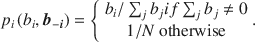
That is, the probability of winning depends on player i’s own bid relative to the sum of all players’ bids, where b _−
i is the vector of bids by all players other than player i. Given (1), the expected payoff for player i, $E (π_{i})$ , can be written as

(2)

E (π_{i}) = p_{i} V + (E - b_{i}) .

The existence and uniqueness of the equilibrium for this game are proved by Szidarovszky and Okuguchi (Reference Szidarovszky and Okuguchi1997) and Chowdhury and Sheremeta (Reference Chowdhury and Sheremeta2011). Following standard procedures, the unique symmetric interior Nash equilibrium bid is

(3)

b^{*} = (N - 1) V / N^{2},

and the expected equilibrium payoff is

(4)

π^{*} = E + V / N^{2} .

In addition, each player also can have a fixed payment, F ≥ 0, that cannot be used in the contest. Hence, F does not affect the equilibrium bid, but is included in the expected payoff and in the equilibrium payoff. We ensure in the experimental design that the available budget is large enough (E > b^*) to obtain an interior solution. Note that the equilibrium bid in Eq. (3) does not depend on individual budget (E), but only on the value of the reward (V) and the number of contestants (N). Hence, as long as the interior equilibrium exists, the standard model predicts that the equilibrium bid is unchanged for any level of budget (E).

3 Experimental procedure and hypothesis

In order to design the experiment in line with our objective, we ran three initial treatments in which we varied the contest budget (E) while keeping everything else the same. There were two parts in each session of each treatment. Part 1 was the same in all sessions. In Part 1, subjects participated in an individual risk elicitation task a la Eckel and Grossman (Reference Eckel and Grossman2008). However, the outcome of the task was not revealed until the end of the experiment. Part 2 was a repeated contest game that differed according to the treatment. Subjects were told that there would be two parts and were given instructions for Part 2 only after everyone had completed Part 1.

In all the treatments, the base game in Part 2 was an individual Tullock contest where three players competed for a reward of 180 tokens, i.e., N = 3 and V = 180. Hence, the risk-neutral equilibrium bid (b ^*), from Eq. 3, was 40 tokens. The contest was repeated for 25 periods in all treatments. The equilibrium remains the same in finite repetitions of the one-shot game. In each period, players received a budget of tokens which they could use to bid for the reward. All players in a session received the same budget in each period. Players could bid any amount from zero to their budget, up to one decimal place. Once all players had entered their bids in a period, they were shown their own bid, the sum of all three bids in their group, whether or not they had won the reward, and their individual earnings from the period. In addition, they were shown a history table with the above information for all previous rounds.

We employed a partner matching protocol, i.e., in each session three subjects were matched into one group of contestants and the matching did not change within a session. This was made clear in the instructions, copies of which are included in Appendix 2 (online). We ran five sessions for each treatment with 18 subjects in a session.Footnote ⁴ In the experimental contests literature, a partner or a random stranger matching protocol is employed interchangeably (Sheremeta Reference Sheremeta2013). We employed a partner matching since it is useful in collecting a sufficient number of independent observations with limited budget. Whereas under random stranger matching the whole session produces only one independent observation, each subject-triple constitutes an independent observation under partner matching. Nonetheless, partner matching can also have drawbacks, since subjects may not employ backward induction correctly, and repeated interaction with the same partners might raise issues of collusion, spite etc. Investigating the effect of matching protocol, Baik et al. (Reference Baik, Chowdhury and Ramalingam2015) find that for 3-player contests these behavioral issues are not prominent, and the choice of matching protocol does not change the bidding behavior in three-player contests. Hence, we safely employ the partner matching protocol in the current study.

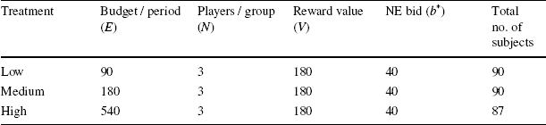
In our three initial treatments, we varied the contest budget (E) available to players. In the ‘Low’ treatment, each subject was given 90 tokens per period which she could use to bid for the reward. The per-period budgets in the ‘Medium’ and ‘High’ treatments were 180 and 540 tokens, respectively. In all the three treatments players received no lump-sum fixed payment, i.e., F = 0. Table 1 summarizes the treatment details.

Table 1 Summary of Treatments

Treatment	Budget / period (E)	Players / group (N)	Reward value (V)	NE bid (b ^*)	Total no. of subjects
Low	90	3	180	40	90
Medium	180	3	180	40	90
High	540	3	180	40	87

Each subject participated in only one of the sessions and did not participate in any contest experiment before. Instructions were read aloud by an experimenter, after which subjects answered a quiz before proceeding to the experiment. While players competed in each of the 25 rounds, they were paid the average earning of five of these rounds chosen randomly (plus the earnings from the risk elicitation task). All subjects in a session were paid for the same five rounds.

The experiment was computerized using z-Tree (Fischbacher Reference Fischbacher2007) and was run in a laboratory of the Centre for Behavioural and Experimental Social Science at the University of East Anglia, UK. The subjects were students at the University and were recruited through the online recruiting system ORSEE (Greiner Reference Greiner2015). Before the payment was made, subject demographic information (age, gender, study area, etc.), and information about their experience in economics experiments were collected through an anonymous survey. Each session took around 1 hour. At the end of each session the token earnings were converted to GBP at the rate of 1 token to 3 Pence. Subjects, on average, earned £13.41.

We denote bids in treatment T as b _T and the budget in treatment T as E _T, where $T = L, M, H$ ; i.e., Low, Medium, High. Note that $V > E_{L} > b^{*}, E_{M} = V > b^{*},$ and $E_{H} > V > b^{*}$ . A hypothesis based on the model above with risk-neutral agents and no decision error shows no difference in bids across the treatments, leading to our null hypothesis below.

Hypothesis The observed bids remain the same as budget increases, i.e., $b_{L} = b_{M} = b_{H} = b^{*} .$

In the following we test this hypothesis with our experimental data. Before we proceed, it is useful to discuss the implications of relaxing the two assumptions we have made. First, it is assumed that agents do not make any errors while making their decisions. If we relax this assumption, considering that the errors are not too expensive and the agents can learn from their errors, one can employ the QRE model to reconsider the effects of the budget. In such a case, as the budget increases, the strategy space also increases and so the scope of making errors. Hence, accordingly to the QRE, an increase in the budget allows a higher degree of error and, as a result, monotonically higher bids.

When players are risk averse, an increase in budget can have two opposing effects. While a higher budget reduces the marginal cost of a bid and encourages higher conflict intensity, a higher budget also reduces the marginal benefit of winning, which discourages conflict intensity. When one considers both the effects together, the overall effect can become ambiguous. In Appendix 1 we present a model with risk averse players and show that an increase in budget has a non-monotonic effect on equilibrium bids. Then, for a specific CRRA utility, we provide a numerical example to show that it is possible to observe an inverted U-shaped relationship between the budget and the bids; i.e., as the budget continue to increase, the first effect (reduction of marginal cost of bid) can be prominent initially while the second effect (reduction of marginal benefit of a win) may become dominant later.

4 Results

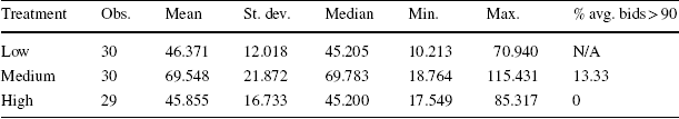
We begin by reporting descriptive statistics of bids by subject-triples (3-subject groups), averaged over the 25 periods and present individual level statistics and analyses later. We do so since a subject triple constitutes an independent observation. Table 2 presents summary statistics of individual bids in each treatment. It also presents the percentage of high average bids (greater than 90, the budget in the Low treatment) observed in each treatment. At first glance it shows that the average bids in all the treatments are over the equilibrium prediction of 40. Moreover, bids are lower in the Low and High treatments with average bids of 46.371 and 45.855 respectively, compared to 69.548 in the Medium treatment.

Table 2 Summary statistics of individual bids per treatment

Treatment	Obs.	Mean	St. dev.	Median	Min.	Max.	% avg. bids > 90
Low	30	46.371	12.018	45.205	10.213	70.940	N/A
Medium	30	69.548	21.872	69.783	18.764	115.431	13.33
High	29	45.855	16.733	45.200	17.549	85.317	0

The number above are for subject triples that make independent observations. The percentage of all individual subject bids that were strictly greater than 90 was 29.11% in Medium and 11.91% in High. The percentage of all individual subject bids that were weakly greater than 90 was 12.44% in Low, 34.49% in Medium and 15.26% in High

Next we test the observations from Table 2 that bids in all three treatments are greater than the equilibrium bid of 40. The p-values for the non-parametric Mann-Whitney Wilcoxon signed rank (z) tests are 0.0030, 0.0001 and 0.1274 for the Low, Medium and High treatments respectively. The tests confirm overbidding in the Low and Medium treatments, but the overbidding is marginally insignificant in the High treatment. This gives our first result.

Result 1 Observed average bids are above equilibrium predictions in all treatments. However, the overbidding is statistically significant only in Low and Medium.

While average bidding behavior—means, medians and fraction of high bids—are similar in Low and High, the standard deviation of bids is higher in the High treatment. This is likely why we do not find evidence of significant overbidding in High. Indeed, as we report below, we do not find significant differences in average bids between Low and High (see Table 3).

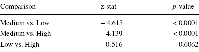
Table 3 Pairwise non-parametric (Wilcoxon rank-sum) tests

Comparison	z-stat	p-value
Medium vs. Low	− 4.613	< 0.0001
Medium vs. High	4.139	< 0.0001
Low vs. High	0.516	0.6062

In terms of dispersion or the spread of the bids, since the strategy space is smaller in the Low treatment compared to the High and the Medium treatments, the standard deviation in the Low treatment is also smaller. In terms of level, a Kruskal-Wallis test confirms difference in bids across treatments (chi-sq with 2 df = 25.818 and p = 0.0001). We now focus on differences in bids between pairs of treatments. Table 3 reports results from the two-sided Mann-Whitney Wilcoxon rank-sum tests. It shows that the bids in the Medium treatment are significantly different from the bids in both High and Low treatments, but that the bids in the latter two treatments are not significantly different from each other. This is reported in the following result.

Result 2 Conflict budget has a non-monotonic effect on the resulting conflict intensity. With an increase in budget from Low to Medium, conflict intensity increases; but with a further increase in budget from Medium to High, conflict intensity decreases.

Result 2 implies that our null hypothesis is clearly rejected. However, the alternative explanation of error (QRE) does not hold for the entire parameter space either. Given QRE, the players incur overbidding by error and the scale of the errors are constrained by the budget of the treatment. Hence, the first part of Result 2, i.e., the increase in bids from Low to Medium can be explained with an error correction model, but not the latter part (a decrease in bids due to an increase in the budget from Medium to High). Thus this alternative hypothesis is rejected.

This result, however, is not an aberration. Chowdhury and Moffatt (Reference Chowdhury and Moffatt2017) run a meta-analysis using the meta data of Sheremeta (Reference Sheremeta2013) comprised of 39 different contest experiments. In their regression the dependent variable is the overbidding rate (bid over the Nash equilibrium level, scaled by the Nash equilibrium bid) and the explanatory variable of interest is the relative endowment (budget size relative to the prize value). They also find an inverted U-shaped relationship between the variables. Hence, the current result is also supported by the meta-data. However, we obtain a clear result of non-monotonic relationship between conflict budget and conflict intensity with a clean experimental design, and are able to control for subject-specific variables. Furthermore, while it is not possible to explain the result using only the meta data, we introduce a further treatment in our study to complement this.

A more credible explanation for the empirical observation (that a very high budget reduces the conflict intensity) might be a wealth effect. Recall that with risk aversion an increase in the budget may reduce the marginal benefit of winning. Hence, when the budget is abundant in the High treatment it can be viewed as wealth, and the marginal benefit from the reward decreases - prompting players to shed their bids. We build a model with risk aversion and run simulation in Appendix 1 to show that indeed such relationship is possible to attain.

To investigate the possibility of such a wealth effect on bidding decisions, we introduce a further treatment titled the ‘Wealth’ treatment. In this treatment subjects received the same per-period budget as in the Medium treatment, 180 tokens, that they could use to bid for the reward. However, each subject also received a one-time lump-sum payment of 360 tokens at the beginning of Part 2, i.e., F = 360. Subjects could not use this amount to bid for the reward. They were told that this was money they had already received as a ‘participation fee’ for this part and that they would be paid this amount in addition to their earnings from the experiment. These details were made clear in the instructions and were again displayed on their screens at the beginning of Part 2. The history screen at the end of every period also contained a reminder of this information. In particular, the following statement was displayed prominently at the top of the history table at the end of each period: “You have already received an initial participation fee of 360 tokens.” Subjects were also reminded of this on their record sheets where they noted down the bids and outcomes each period. The details of the treatment are included in Table 4 along with the Medium treatment.

Table 4 Wealth Treatment

Treatment	Budget / period (E)	Fixed Fee (F)	Players / group (N)	Reward value (V)	Eqbm bid (b ^*)	Total no. of subjects
Medium	180	0	3	180	40	90
Wealth	180	360	3	180	40	90

The risk-neutral Nash equilibrium bid and the strategy space are not affected by the introduction of this fixed payment (F), and remain the same as in the Medium treatment.Footnote ⁵ Hence, in absence of any wealth effect, one would expect the same bidding behavior in this treatment as in the Medium treatment. However, in presence of a wealth effect, as explained earlier, one should expect the bidding behavior to be more comparable to that of the High treatment.

Note that we only paid subjects in the Wealth treatment the participation fee of 360 tokens once, but reminded them of the same in every period. Another way this treatment could be implemented is to pay the fee of 360 tokens in each period. As framing may affect decision making, it is an empirical question which of the two versions of the Wealth treatments is more appropriate to implement. We decided to implement the current version of the Wealth treatment.

The average bid in the Wealth treatment is 46.639 tokens with a standard deviation of 16.607. The minimum and maximum (average) individual bids in the Wealth treatment in a period are 11.105 and 71.453 respectively. Comparing this with Table 2 (which shows that the average bids in the Low, Medium and High treatments are 46.371, 69.548, and 45.855) it indeed appears that the average bids are more comparable in the High and the Wealth treatments, but they are different when we consider the Wealth and the Medium treatments.

To test the statistical significance of these results, a Kruskal-Wallis test for joint difference among all 4 treatments confirms difference in distributions (p = 0.0001). Moreover, Table 5 reports the results of pairwise Wilcoxon rank-sum tests that investigate whether bids in the Wealth treatment are different from bids in the other three treatments. It confirms that average bids in the High and Wealth treatments (and High and Low) are not significantly different, but average bids in Medium are significantly different than in the Wealth treatment. This provides an explanation for Result 2 and confirms that the high level of budget in the High treatment has a net wealth effect that presumably reduces the marginal benefit of winning; and, as a result, reducing the bids.

Table 5 Non-parametric (Wilcoxon rank-sum) tests of pairwise comparison

Comparison	z-stat	p-value
Medium vs. Wealth	4.214	0.0000
High vs. Wealth	− 0.576	0.5645
Low vs. Wealth	− 0.296	0.7675

These results are obtained at the independent observation (i.e., subject-triple) level, and thus are highly aggregated. Previous evidence shows in individual Tullock contests that there is significant evolution of bidding behavior over time—namely, bids are usually decreasing over time (Dechenaux et al. Reference Dechenaux, Kovenock and Sheremeta2015). Evidences also point to significant heterogeneity in the (average) bids of individuals, i.e., bids have been seen to have a wide dispersion over the action space (Chowdhury et al. Reference Chowdhury, Sheremeta and Turocy2014; Dechenaux et al. Reference Dechenaux, Kovenock and Sheremeta2015). We next graphically explore such differences in time-trends and heterogeneity across treatments. Figure 1 presents average individual bids over the bid range and over time in all treatments.

Fig. 1 Average individual bids over bid range and over time

The left panel of Fig. 1 shows the distribution of average individual bids across the bid range by treatments. Note that for Low treatment the maximum bid can be 90, whereas it is higher for the other three treatments. For each treatment most of the bids are concentrated between 40 and 80 and there are only a few bids made at the reward value (180). Observe also that bids in the higher range are more frequent in the Medium treatment than the other three. To examine whether the bids are concentrated in particular periods, the right panel plots the average individual bids over periods. Overall it supports the previous findings that for all treatments bids go down over time, but still stay over the equilibrium bid. Further, it confirms the ranking of treatments observed above over the entire time range.

The analyses thus far concentrated on subject-triple bids or individual bids, but did not control for any other relevant factors such as repeated games dynamics, or subjects’ demographic characteristics. Although isolating the analysis from these factors may still provide important information about treatment effects, it is important to test the robustness of the results to such controls. Hence, to test whether these results are robust at the individual level, Table 6 presents random effects panel regressions of individual bid in a period on treatment dummies, our main variables of interest. However, we also control for other possible factors. The first set includes the standard repeated contests controls (Dechenaux et al. Reference Dechenaux, Kovenock and Sheremeta2015) for past outcomes within the triple: the individual’s bid in the previous period, an indicator for whether or not the individual won the contest in the previous period, and the sum of the bids of the others in the triple in the previous period. We further control for an individual’s demographic characteristics: an indicator for risky behavior,Footnote ⁶ an indicator for a graduate student (i.e., if age ≥ 21 years), a female gender dummy and the number of experiments the individual has participated in in the past (experience). We report robust standard errors clustered on independent triples.

Table 6 Comparisons of treatments

Dep Var: b _it	(1)	(2)
Dep Var: b _it	No demographic controls	With demographic controls
Lag bid	0.495^***	0.493^***
Lag bid	(0.0301)	(0.0299)
Lag win	1.837^*	1.700^*
Lag win	(1.024)	(1.023)
Lag others bid	0.0425^***	0.0429^***
Lag others bid	(0.0157)	(0.0155)
Period	− 0.125^**	− 0.126^**
Period	(0.0538)	(0.0540)
Low	− 9.488^***	− 9.409^***
Low	(2.128)	(2.142)
High	− 10.49^***	− 10.81^***
High	(2.226)	(2.242)
Wealth	− 9.774^***	− 9.980^***
Wealth	(2.238)	(2.237)
Risky behavior	–	− 0.0875
Risky behavior		(1.426)
Age ≥ 21	–	− 0.235^*
Age ≥ 21		(0.133)
Female	–	2.037
Female		(1.585)
Experience	–	0.186
Experience		(0.131)
Constant	30.29^***	33.72^***
Constant	(3.208)	(4.409)
Observations	8568	8568

Dependent variable: Individual bid in each period. Robust standard errors clustered on independent subject-triples (groups) are in parentheses

^* p < 0.10

^** p < 0.05

^*** p < 0.01

The first column in Table 6 reports a regression with dynamic game controls in which the baseline treatment is Medium. As expected, we find that compared to Medium all the treatments significantly reduce individual bids. The dynamic game controls show signs in line with the existing literature. The next column reports the same regression, but also with demographic controls. The direction and significance of the results remain the same and only age turns out to be significant. The regressions reaffirm that the result of the non-monotonic effect of conflict budget is robust; and that individual bids are lower with wealth, i.e., when subjects are richer.

Although the regression results confirm that individual bids in Medium are higher than in all the other three treatments, they do not directly corroborate whether the bids in the Wealth treatment are different from those in the High treatment. To investigate this, we run (pairwise) post-regression tests for differences among Low, Medium and Wealth. For both the regressions, the tests results show that there is no significant difference among bids in Low, Medium and Wealth treatments (p > 0.35 for each of these tests).Footnote ⁷ The outcomes from Tables 3, 5, and 6 along with the explanations are summarized in the following result.

Result 3 When the budget is scarce, an increase in the budget increases conflict intensity. However, when the budget is abundant, or the budget is combined with added wealth, then conflict intensity decreases with a further increase in budgets.

Our results provide a common platform for both the opposing results discussed in the literature. It shows that conflict budget can have counteracting effects, and one effect may dominate the other in different situations. From Low to Medium, an increase in the budget allows for higher level of error and that can increase conflict intensity. It may also reduce the marginal cost of bidding, thus increasing bids. However, from Medium to High, the budget is viewed as wealth and the marginal benefit of winning the prize becomes lower—resulting in lower bids.

Although it is not the primary focus of our analysis, it is useful to investigate any possible treatment effect on dispersion or overspreading of bids (Chowdhury et al. Reference Chowdhury, Sheremeta and Turocy2014). If the spreads are very different across treatments, then it will warrant further investigation in this context. We find that only Medium and Low have a marginally significant difference (p = 0.08) in standard deviations (since Low has a smaller strategy space) and no other significant differences can be observed. We, hence, conclude that the heterogeneous overspreading is not an issue in this experiment.

5 Discussion

We investigate the effects of conflict budget on conflict intensity. We run a between-subject Tullock (Reference Tullock, Buchanan, Tollison and Tullock1980) contest experiment in which we systematically vary the budget that can be used in the experimental task while keeping the Nash equilibrium bid the same across treatments. The bids in the contest reflect the conflict intensity. Existing experimental results observe an increase in contest bids due to an increase in the budget and explain this with an error correction model: with higher budget the strategy space increases and the subjects make more mistakes. However, a negative relationship between budget and conflict intensity has also been observed empirically in various circumstances.

Our results show that, ceteris paribus, when the budget is increased from Low to Medium, bids increase. However, when the budget is increased further from Medium to High, bids decrease. The first part of the result matches with that in Sheremeta (Reference Sheremeta2010, Reference Sheremeta2011), and can be explained with error correction models such as the QRE. But such error correction models cannot explain the second part of the result in which bids decrease with an increase in the budget.

Our result, however, is reminiscent of the ‘backward bending supply curve of labor’ (Pigou Reference Pigou1920), which suggests that as the wage rate increases, labor supply will first increase and when the wage rate is sufficiently high, the labor supply will decrease. This was later supported in a laboratory experiment by Dickinson (Reference Dickinson1999). The majority of the literature explains this phenomenon with the diminishing marginal utility of income.

In the same spirit, when the players are risk averse, an increase in the budget can have two countervailing effects on conflict behavior. If one has a higher budget, then it is relatively easier for her to bid one more unit as the (marginal) opportunity cost of bidding becomes low. This should result in an increase in bids as budget increases. At the same time this higher budget can be viewed as wealth and in such a case, earning the reward provides less marginal utility compared to when the budget is low, decreasing the marginal benefit of winning. This second factor results in a decrease in bidding. Our apparently puzzling result of a non-monotonic effect of the budget on bids can be explained if the second factor dominates the first factor. We show, with a numerical example, that it may indeed be possible to obtain such a result. We then investigate this by introducing another treatment in which the budget remains moderate, but subjects are given a fixed payment (wealth) that cannot be used in conflict. It turns out that the conflict intensity in this treatment is not different from that in the high budget treatment.

There are several implications of this result. First, contributing to the conflict literature, for the same value of a reward (a crucial assumption in our setting), one would expect to observe more conflict in medium income societies than in poor or rich societies. Hirshleifer (Reference Hirshleifer, Hartley and Sandler1995), in a very different setting, states that conflict is a more attractive option for the relatively poorer individuals. We extend this argument by showing that even without an option for production, a very high budget may result in less conflict due to a wealth effect. Hence, ceteris paribus, the availability of a higher budget for conflict would not necessarily monotonically escalate the intensity of conflict. Our result also contributes to the contest literature by showing that when a wealth effect is strong, the existing results might change.

Second, an implication of the result from the Wealth treatment is that subject behavior may be affected by the introduction, and the amount of a fixed fee, in the experiment. This can be a methodologically troublesome finding because different laboratories use different fees, and even within the same laboratory fees may differ depending on the duration of the experiment. This effect is already recognized in other areas of research such as social preferences (Korenok et al. Reference Korenok, Millner and Razzolini2013; Chowdhury and Jeon Reference Chowdhury and Jeon2014) or social dilemmas (Clark Reference Clark2002). We contribute to the literature of the effects of fixed-fee on experimental subjects’ behavior by extending it to a contest game. It may still be possible to find clear and robust treatment effects in contest experiments if the aim is not focused on the fixed fee, but our result indicates the need for further investigation in this area.

Our results also indicate a well-known anomaly. Although the model with risk aversion can explain the empirical finding, we find no significance of the risk attitude variable (Table 6). Hence, it may be the case that our specific measure of risk attitude (Eckel and Grossman Reference Eckel and Grossman2008) could not estimate the effects of risk aversion and a different measure may have been appropriate.

It is possible to extend this research in various interesting avenues. Since wealth or budget change symmetrically in our experiment, a natural next step would be to investigate if wealth or budget inequality increases or decreases conflict. It would also be interesting to test the effects of changes in wealth on conflict intensity. A specifically designed experiment replicating the two countervailing effects as mentioned above would contribute nicely to the literature. The interaction of wealth and loss aversion (Chowdhury et al. Reference Chowdhury, Jeon and Ramalingam2018) may also be interesting. Finally, it would be worthwhile investigating such issues with field data.

Acknowledgements

We thank David Cooper (Editor), two anonymous referees, Daniel Arce, Paul Gorny, Kai Konrad, John Morgan, Curtis Price, Roman Sheremeta, Georgios Papadopoulos, Ted Turocy, Michela Vecchi, the participants at the SAET conference in Cambridge, Conflict Research Society conference in Kent, European ESA meetings in Prague, and seminar participants at East Anglia, Essex, Groningen, Institute of Development Studies (Kolkata), Korea, and Middlesex for comments. Any remaining errors are our own.

Appendix 1: A model with risk aversion

Here we present a model with risk-aversion and show the effects of an increase in wealth or budget. First, with an $N$ -player model we establish a non-monotonic relationship between budget and bid. Then, commensurate to our experiment, in a 3-player case (with a specific CRRA utility function), we show that an inverted U-shaped relationship may be possible with a numerical example.

Suppose player $i$ (where $i \in S = (1, 2, \dots, N)$ ) has the thrice differentiable utility function $u_{i} (π_{i})$ with the property $u_{i}^{^{'}} \geq 0, u_{i}^{^{''}} < 0$ . The expected utility is:

\begin{matrix} E (u_{i}) = p_{i} u_{i} (V + E_{T} - b_{i}) + (1 - p_{i}) u_{i} (E_{T} - b_{i}) \\ = p_{i} (u_{i} (V + E_{T} - b_{i}) - u_{i} (E_{T} - b_{i})) + u_{i} (E_{T} - b_{i}) \end{matrix}

where $b_{i}$ is the bid, $p_{i}$ is the probability of winning of player $i$ ; $V$ is the common prize value and $E_{T}$ is the budget in treatment $T$ . The function is concave, and the first order condition shows:

\begin{matrix} \frac{\partial E (u_{i})}{\partial b_{i}} = p_{i}^{^{'}} (u_{i} (V + E_{T} - b_{i}) - u_{i} (E_{T} - b_{i})) + p_{i} (- u_{i}^{^{'}} (V + E_{T} - b_{i}) + u_{i}^{^{'}} (E_{T} - b_{i})) - u_{i}^{^{'}} (E_{T} - b_{i}) \\ = p_{i}^{^{'}} (u_{i} (V + E_{T} - b_{i}) - u_{i} (E_{T} - b_{i})) - (p_{i} u_{i}^{^{'}} (V + E_{T} - b_{i}) + (1 - p_{i}) u_{i}^{^{'}} (E_{T} - b_{i})) = 0 \end{matrix}

Implementing the Tullock CSF ( $p_{i} = b_{i} / (\sum b_{i})$ ), we get:

\frac{\partial E (u_{i})}{\partial b_{i}} = \frac{\sum_{j \in (S \ i)} b_{j}}{{(\sum b_{i})}^{2}} (u_{i} (V + E_{T} - b_{i}) - u_{i} (E_{T} - b_{i})) - (\frac{b_{i}}{\sum b_{i}} u_{i}^{^{'}} (V + E_{T} - b_{i}) + \frac{\sum_{j \in (S \ i)} b_{j}}{\sum b_{i}} u_{i}^{^{'}} (E_{T} - b_{i})) = 0

Now, considering the symmetric equilibrium ( $b_{i} = b_{j} = b^{*}$ ), this yields:

(5)

\frac{(n - 1)}{n^{2} b^{*}} (u_{i} (V + E_{T} - b^{*}) - u_{i} (E_{T} - b^{*})) - (\frac{1}{n} u_{i}^{^{'}} (V + E_{T} - b^{*}) + \frac{(n - 1)}{n} u_{i}^{^{'}} (E_{T} - b^{*})) = 0

Let us elaborate on Eq. (5) to show the effects of the budget. Differentiating it with $E_{T}$ , which is equivalent to adding $F$ , we get:

\begin{matrix} - \frac{(N - 1)}{N^{2} b^{* 2}} \frac{\partial b^{*}}{\partial E_{T}} (u_{i} (V + E_{T} - b^{*}) - u_{i} (E_{T} - b^{*})) + \frac{(N - 1)}{N^{2} b^{*}} (u_{i}^{^{'}} (V + E_{T} - b^{*}) (1 - \frac{\partial b^{*}}{\partial E_{T}}) - u_{i}^{^{'}} (E_{T} - b^{*}) (1 - \frac{\partial b^{*}}{\partial E_{T}})) \\ - \frac{1}{N} (u_{i}^{^{''}} (V + E_{T} - b^{*}) (1 - \frac{\partial b^{*}}{\partial E_{T}}) + (N - 1) u_{i}^{^{''}} (E_{T} - b^{*}) (1 - \frac{\partial b^{*}}{\partial E_{T}})) = 0 \end{matrix}

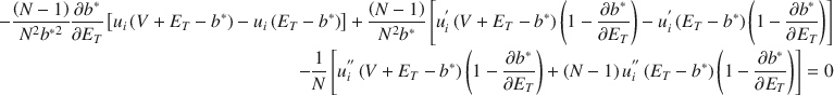
After rearranging terms, we get:

\frac{\partial b^{*}}{\partial E_{T}} = \frac{\frac{(N - 1)}{N^{2} b^{*}} u_{i}^{'} (V + E_{T} - b^{*}) - \frac{(N - 1)}{N^{2} b^{*}} u_{i}^{'} (E_{T} - b^{*}) - \frac{1}{N} u_{i}^{″} (V + E_{T} - b^{*}) - \frac{(N - 1)}{N} u_{i}^{″} (E_{T} - b^{*})}{\frac{(N - 1)}{N^{2} b^{* 2}} (u_{i} (V + E_{T} - b^{*}) - u_{i} (E_{T} - b^{*})) + \frac{(N - 1)}{N^{2} b^{*}} u_{i}^{'} (V + E_{T} - b^{*}) - \frac{(N - 1)}{N^{2} b^{*}} u_{i}^{'} (E_{T} - b^{*}) - \frac{1}{N} u_{i}^{″} (V + E_{T} - b^{*}) - \frac{(N - 1)}{N} u_{i}^{″} (E_{T} - b^{*})}

Now employing Eq. (5) in the denominator, and further rearranging yields:

\frac{\partial b^{*}}{\partial E_{T}} = \frac{1}{N} \frac{(N - 1) u_{i}^{'} (V + E_{T} - b^{*}) - (N - 1) u_{i}^{'} (E_{T} - b^{*}) - N b^{*} u_{i}^{″} (V + E_{T} - b^{*}) - N (N - 1) b^{*} u_{i}^{″} (E_{T} - b^{*})}{\frac{(2 N - 1)}{N} u_{i}^{'} (V + E_{T} - b^{*}) + \frac{{(N - 1)}^{2}}{N} u_{i}^{'} (E_{T} - b^{*}) - b^{*} u_{i}^{″} (V + E_{T} - b^{*}) - b^{*} (N - 1) u_{i}^{″} (E_{T} - b^{*})}

Note that given $u_{i}^{'} \geq 0, and u_{i}^{″} < 0$ , the denominator of the right-hand-side is always positive. Hence, the sign of $\frac{\partial b^{*}}{\partial E_{T}}$ depends on the sign of the numerator. In particular:

(6)

\frac{\partial b^{*}}{\partial E_{T}} (\begin{matrix} > 0 i f (N - 1) (u_{i}^{'} (V + E_{T} - b^{*}) - u_{i}^{'} (E_{T} - b^{*})) > N b^{*} (u_{i}^{″} (V + E_{T} - b^{*}) + (N - 1) u_{i}^{″} (E_{T} - b^{*})) \\ = 0 i f (n - 1) (u_{i}^{'} (V + E_{T} - b^{*}) - u_{i}^{'} (E_{T} - b^{*})) = N b^{*} (u_{i}^{″} (V + E_{T} - b^{*}) + (N - 1) u_{i}^{″} (E_{T} - b^{*})) \\ < 0 i f (n - 1) (u_{i}^{'} (V + E_{T} - b^{*}) - u_{i}^{'} (E_{T} - b^{*})) < N b^{*} (u_{i}^{″} (V + E_{T} - b^{*}) + (N - 1) u_{i}^{″} (E_{T} - b^{*})) \end{matrix})

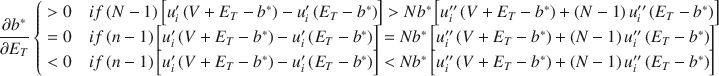
Equation (6) states that equilibrium bid may eventually reduce as the budget increases, but it will depend on the specific utility function and the corresponding parameter values.

We now show the possibility of an inverted U-shape relationship between budget and bid with a numerical example with three players (N = 3) that matches with our experimental design. Note that for any such example, Eq. (5) should hold $.$ Suppose that player $i$ has an ordinal CRRA utility function: $u_{i} (π) = \frac{π^{(1 - γ)}}{(1 - γ)}$ with $γ > 0;$ hence, $u_{i}^{^{'}} (π) = π^{- γ}$ and $u_{i}^{^{''}} (π) = - γ {(π)}^{- (1 + γ)}$ .

Now consider two cases. In both the cases the utility function and the valuation remains the same ( $V = 100$ and $γ = 5$ ). However, the first case represents a lower budget while the second one represents a higher budget. Then we calculate both the equilibrium bid and the change in the equilibrium bid (due to a change in the budget).

Case 1 $E_{T} = 1982$ ; then from Eq. (5): $b \approx 21.2216813891606$ . Also, from Eq. (6): $\frac{\partial b^{*}}{\partial E_{T}} = 0.000570254 > 0$ .

Case 2 $E_{T} = 2360$ ; then from Eq. (5): $b \approx 21.18912426$ . Also, from Eq. (6): $\frac{\partial b^{*}}{\partial E_{T}} = - 0.0000306434247669666 < 0$ .

Hence, in this numerical example, Case 1 reflects the first part of the inverted U-shape we have obtained in our experimental data where an increase in the budget increases the bids. Case 2, on the other hand, reflects the second part where an increase in the budget decreases the bids.

We further run the same procedure for several other budget values (1970, 1982, 1998 - for which the bid increases with budget and the slope is positive; and 2350, 2360, 2402 - for which the bid decreases with budget and the slope is negative) and plot the equilibrium bids ( $b^{*}$ ) against the budget ( $E_{T}$ ) in Fig. 2.

Fig. 2 Bids against budget

This shows the possibility of an inverted U-shaped relationship between budget and the level of conflict. Note that in the example above the budget value needs to be relatively high in order to obtain the negative slope. This is due to the of the specific CRRA (constant relative risk aversion) utility function used. It may also be possible for other parametric values that other shape of such relationship is obtained. Nevertheless, this example still provides the required intuition behind the non-monotonic relationship obtained in the experimental data.

Footnotes

Electronic supplementary material The online version of this article (https://doi.org/10.1007/s10683-019-09615-0) contains supplementary material, which is available to authorized users.

¹ Ciccone (Reference Ciccone2011), however, employs an alternative empirical method in the same data and finds no such relationship.

² Although several studies in contest experiments term the budget as ‘endowment’, we refrain from doing so in order to avoid any confusion with the psychological endowment effect (Thaler Reference Thaler1980; Kahneman Kahneman et al. Reference Kahneman, Knetsch and Thaler1991).

³ There is a large body of evidence on overbidding relative to the equilibrium in contest experiments. This phenomenon is attributed to many possible reasons such as the joy of winning (Sheremeta Reference Sheremeta2010), bounded rationality (Sheremeta Reference Sheremeta2011; Chowdhury et al. Reference Chowdhury, Sheremeta and Turocy2014), player heterogeneity (Herbst et al. Reference Herbst, Konrad and Morath2015), lack of understanding of probability etc. See Sheremeta (Reference Sheremeta2013) and Dechenaux et al. (Reference Dechenaux, Kovenock and Sheremeta2015)for surveys on this issue.

⁴ Due to lower than expected show-up, a session in the High treatment had only 15 subjects. Hence, we have 30 triples for the Low and the Medium treatments and 29 triples for the High treatment. Given the partner matching design, each triple constitutes an independent observation.

⁵ Additionally, since, as in the Medium treatment, the budget per period is the same as the reward value, the Wealth treatment also controls for any possible ‘focality’ that the subjects may have in the Medium treatment.

⁶ The risk elicitation task had six options (1–6) in increasing order of risk: see Instructions Part 1 in Appendix 2 (online). The risky behavior indicator takes the value 1 for subjects who chose option 4–6, and 0 otherwise. The results are robust to alternative definitions of the indicator.

⁷ We also run regressions that compare pairwise the bids in different treatments. All the results reported above are still supported with the pairwise regressions. The regression results are available from the authors upon request.

Springer Nature remains neutral with regard to jurisdictional claims in published maps and institutional affiliations.

References

Baik, K. H., Chowdhury, S. M. & Ramalingam, A. (2015). Group Size and Matching Protocol in Contests. University of East Anglia CBESS Discussion Paper No. 13-11R.Google Scholar

Becker, GS (1983). A theory of competition among pressure groups for political influence. Quarterly Journal of Economics, 98(3), 371–400. 10.2307/1886017CrossRef Google Scholar

Bosch-Domènech, A, Silvestre, J Schultz, C, & Vind, K (2006). Do the wealthy risk more money? An experimental comparison. Institutions, equilibria and efficiency: essays in honor of Birgit Grodal, Berlin: Springer 95–106. 10.1007/3-540-28161-4_6CrossRef Google Scholar

Che, YK, & Gale, I (1997). Rent dissipation when rent seekers are budget constrained. Public Choice, 92(1–2), 109–126. 10.1023/A:1017937708549CrossRef Google Scholar

Che, YK, & Gale, IL (1998). Caps on political Lobbying. American Economic Review, 88(3), 643–651.Google Scholar

Chowdhury, SM, & Jeon, J (2014). Impure altruism or inequality aversion?: An experimental investigation based on income effects. Journal of Public Economics, 118, 143–150. 10.1016/j.jpubeco.2014.07.003CrossRef Google Scholar

Chowdhury, SM, Jeon, JY, & Ramalingam, A (2018). Property rights and loss aversion in contests. Economic Inquiry, 56(3), 1492–1511. 10.1111/ecin.12505CrossRef Google Scholar

Chowdhury, SM, & Moffatt, PG (2017). Overbidding and heterogeneous behavior in contest experiments: A comment on the endowment effect. Journal of Economic Surveys, 31(2), 572–576. 10.1111/joes.12152CrossRef Google Scholar

Chowdhury, SM, & Sheremeta, RM (2011). Multiple equilibria in Tullock contests. Economics Letters, 112(2), 216–219. 10.1016/j.econlet.2011.05.002CrossRef Google Scholar

Chowdhury, SM, Sheremeta, RM, & Turocy, TL (2014). Overbidding and overspreading in rent-seeking experiments: Cost structure and prize allocation rules. Games and Economic Behavior, 87, 224–238. 10.1016/j.geb.2014.05.004CrossRef Google Scholar

Ciccone, A (2011). Economic Shocks and civil conflict: A comment. American Economic Journal: Applied Economics, 3(4), 215–227.Google Scholar

Clark, J (2002). House money effects in public good experiments. Experimental Economics, 5(3), 223–231. 10.1023/A:1020832203804CrossRef Google Scholar

Cornes, R, & Hartley, R (2003). Risk aversion, heterogeneity and contests. Public Choice, 117(1–2), 1–25. 10.1023/A:1026136008608CrossRef Google Scholar

Cornes, R, & Hartley, R (2012). Risk aversion in symmetric and asymmetric contests. Economic Theory, 51(2), 247–275. 10.1007/s00199-009-0490-9CrossRef Google Scholar

Dechenaux, E, Kovenock, D, & Sheremeta, RM (2015). A survey of experimental research on contests, all-pay auctions and tournaments. Experimental Economics, 18(4), 609–669. 10.1007/s10683-014-9421-0CrossRef Google Scholar

Dickinson, DL (1999). An experimental examination of labor supply and work intensities. Journal of Labor Economics, 17(4), 638–670. 10.1086/209934CrossRef Google Scholar

Durham, Y, Hirshleifer, J, & Smith, VL (1998). Do the rich get richer and the poor poorer? Experimental tests of a model of power. American Economic Review, 88(4), 970–983.Google Scholar

Eckel, CC, & Grossman, PJ (2008). Forecasting risk attitudes: An experimental study using actual and forecast gamble choices. Journal of Economic Behavior & Organization, 68(1), 1–17. 10.1016/j.jebo.2008.04.006CrossRef Google Scholar

Fischbacher, U (2007). z-Tree: Zurich toolbox for ready-made economic experiments. Experimental Economics, 10(2), 171–178. 10.1007/s10683-006-9159-4CrossRef Google Scholar

Greiner, B (2015). Subject pool recruitment procedures: Organizing experiments with ORSEE. Journal of the Economic Science Association, 1(1), 114–125. 10.1007/s40881-015-0004-4CrossRef Google Scholar

Herbst, L, Konrad, KA, & Morath, F (2015). Endogenous group formation in experimental contests. European Economic Review, 74, 163–189. 10.1016/j.euroecorev.2014.12.001CrossRef Google Scholar

Hirshleifer, J (1991). The paradox of power. Economics and Politics, 3(3), 177–200. 10.1111/j.1468-0343.1991.tb00046.xCrossRef Google Scholar

Hirshleifer, J. (1995). Theorizing about conflict. In Hartley, K. Sandler, T. (Eds.), Handbook of defense economics (Vol. 1, pp. 165–189). Amsterdam: North-Holland.Google Scholar

Kahneman, D, Knetsch, JL, & Thaler, RH (1991). Anomalies: the endowment effect, loss aversion, and status quo bias. Journal of Economic Perspectives, 5(1), 193–206. 10.1257/jep.5.1.193CrossRef Google Scholar

Kocher, M, Martinsson, P, & Visser, M (2008). Does stake size matter for cooperation and punishment?. Economics Letters, 99, 508–511. 10.1016/j.econlet.2007.09.048CrossRef Google Scholar

Konrad, KA (2009). Strategy and dynamics in contest, Oxford: Oxford University Press.CrossRef Google Scholar

Konrad, KA, & Schlesinger, H (1997). Risk aversion in rent-seeking and rent-augmenting games. The Economic Journal, 107(445), 1671–1683. 10.1111/j.1468-0297.1997.tb00074.xCrossRef Google Scholar

Korenok, O, Millner, EL, & Razzolini, L (2013). Impure altruism in dictators’ giving. Journal of Public Economics, 97, 1–8. 10.1016/j.jpubeco.2012.08.006CrossRef Google Scholar

McKelvey, R, & Palfrey, T (1995). Quantal response equilibria for normal form games. Games and Economic Behavior, 10(1), 6–38. 10.1006/game.1995.1023CrossRef Google Scholar

Miguel, E, Satyanath, S, & Sergenti, E (2004). Economic shocks and civil conflict: An instrumental variables approach. Journal of Political Economy, 112(4), 725–753. 10.1086/421174CrossRef Google Scholar

Morgan, J, Orzen, H, & Sefton, M (2012). Endogenous entry in contests. Economic Theory, 51(2), 435–463. 10.1007/s00199-010-0544-zCrossRef Google Scholar

Pigou, AC (1920). The economics of welfare part I, New York: Cosimo Classics.Google Scholar

Price, CR, & Sheremeta, RM (2011). Endowment effects in contests. Economics Letters, 111, 217–219. 10.1016/j.econlet.2011.02.003CrossRef Google Scholar

Schroyen, F, & Treich, N (2016). The power of money: wealth effects in contests. Games and Economic Behavior, 100, 46–68. 10.1016/j.geb.2016.09.005CrossRef Google Scholar

Sheremeta, RM (2010). Experimental comparison of multi-stage and one-stage contests. Games and Economic Behavior, 68(2), 731–747. 10.1016/j.geb.2009.08.001CrossRef Google Scholar

Sheremeta, RM (2011). Contest design: An experimental investigation. Economic Inquiry, 49(2), 573–590. 10.1111/j.1465-7295.2009.00274.xCrossRef Google Scholar

Sheremeta, RM (2013). Overbidding and heterogeneous behavior in contest experiments. Journal of Economic Surveys, 27, 491–514. 10.1111/joes.12022CrossRef Google Scholar

Szidarovszky, F, & Okuguchi, K (1997). On the existence and uniqueness of pure nash equilibrium in rent-seeking games. Games and Economic Behavior, 18, 135–140. 10.1006/game.1997.0517CrossRef Google Scholar

Thaler, R (1980). Toward a positive theory of consumer choice. Journal of Economic Behavior & Organization, 1(1), 39–60. 10.1016/0167-2681(80)90051-7CrossRef Google Scholar

Tullock, G Buchanan, JM, Tollison, RD, & Tullock, G (1980). Efficient rent seeking. Toward a theory of the rent-seeking society, College Station: Texas A&M University Press 97–112.Google Scholar