


1 Introduction
When investigating the functioning of markets one is puzzled by the huge variety of market institutions used to trade similar or even the same good (see e.g. Madhavan Reference Madhavan1992; Quan Reference Quan1994; Zumpano et al. Reference Zumpano, Elder and Baryla1996). Extensive research has revealed that the institutional rules governing trade have a substantial impact on prices, quantities, and the resulting efficiency of markets (see, among many others, Lucking-Reiley Reference Lucking-Reiley2000; Reynolds and Wooders Reference Reynolds and Wooders2009; Ariely et al. Reference Ariely, Ockenfels and Roth2005; Ausubel et al. Reference Ausubel, Cramton, Pycia, Rostek and Weretka2014; Genesove and Hansen Reference Genesove and Hansen2016). This in turn led to substantial research on the evolution of market rules (see e.g. Rud and Rabanal Reference Rud and Rabanal2018). Starting with the seminal contribution of Hayek (Reference Hayek1967) it has been argued that traders, if left to their own devices, choose the most efficient trading institution that the good at hand allows for.Footnote 1 This article aims to test this conjecture experimentally. Specifically, we set out to investigate whether efficient institutions are indeed used in the long run, while inefficient ones fade as they are eventually avoided by the traders.
Take a situation where different trading platforms are feasible for trading a particular good. Each trader has to choose which one he/she wants to use.Footnote 2 An individual buyer or seller will not choose a platform where he/she cannot find a trading partner, even if the institutional setup of the avoided platform would lead to very efficient trading outcomes. Hence, traders face a (partial) coordination game when choosing on which platform they want to trade.Footnote 3 After choosing the trading institution, i.e. for a given distribution of buyers and sellers over the feasible platforms, the institutional setups–together with demand and supply resulting from the platform choice–will lead to more or less efficient trading outcomes. Hence, the whole process is characterized by two steps: First, traders have to choose the trading platform (where to trade). Then, they conduct their trades with the partners available at their platform (how much and at which price to trade).
In our experiment each subject is either a buyer or a seller. In the first stage of each experimental round, each subject had to choose individually between a posted offer (PO; with sellers posting prices) institution and an open double auction (DA, Plott and Gray Reference Plott and Gray1990; “open” meaning that there was no auctioneer, thus multiple prices could be realized).Footnote 4 In the second stage of each round, subjects could trade multiple units of a homogeneous good according to the rules of the chosen institution with those potential trading partners who had opted for the same institution. At the end of each round, all the participants received aggregate information about what happened at both institutions, enabling them to make an informed decision on where to trade in the next round: number of buyers and sellers, distribution of trading prices (and their average), and number of trades per buyer and per seller at each institution. Then a new round started, where first all subjects had to choose between the DA and the PO. After that, they traded on the chosen platform anew, received information about the outcome of both institutions, and so on.
For each trade conducted, the seller received the price paid by the buyer, but in turn she had to pay production costs that were determined by the experimental design. Hence, her net earnings from a trade were the difference between the price and production costs. For a buyer, the net earnings from a trade were the difference between the resale values, which were determined by the design of the experiment, and the price paid.Footnote 5 That is, in each given round, the actual, endogenously-induced supply and demand at a given platform was determined by the production costs and resale values of the sellers and buyers who opted for that platform. To keep the demand and supply functions constant, and since our focus is on which institutions survive, the induced values were the same for all buyers and the production costs were the same for all sellers.
We chose DA and PO as institutional alternatives since it is very well documented that, when functioning in isolation, DAs are highly efficient, whereas POs tend to create inefficiencies and are biased towards sellers. Theoretically, for example, Rustichini et al. (Reference Rustichini, Satterthwaite and Williams1994) show that, in double auctions, possible inefficiencies due to traders’ strategic misreporting vanish quickly as the number of traders increase. Empirically, it has been repeatedly shown that DAs induce a very quick convergence of prices and quantities to market clearing levels (see, e.g., the seminal article of Plott and Smith Reference Plott and Smith1978a). As a consequence, the DA has been found to be the most efficient market institution when efficiency is measured by the sum of all gains from trade reaped by buyers and sellers (as it is usually done in the context of market experiments). In fact, DA is routinely used in market experiments as a proxy for competitive markets (e.g., Plott Reference Plott2000; Crockett et al. Reference Crockett, Oprea and Plott2011; Gillen et al. Reference Gillen, Hirota, Hsu, Plott and Rogers2020). On the other hand, in the PO prices and quantities typically show a much slower convergence to the market clearing level, with prices typically converging from above (see Plott and Smith Reference Plott and Smith1978a). For given demand and supply, the efficiency level is considerably higher for a DA than for a PO. If efficiency drives the selection of market institutions, we should expect that traders coordinate on the DA, and that the PO eventually falls into disuse.
The experimental results indicate that the validity of this prediction depends crucially on the properties of the distribution of production costs. If the production technology underlying the sellers’ supply function exhibits decreasing returns to scale, traders indeed learn to coordinate on the efficient DA, with PO becoming mostly inactive in finitely many rounds. In contrast, if production displays constant returns to scale, resulting in a flat induced supply function, coordination on DA happens more slowly and both institutions remain active until the last round.Footnote 6 This difference might be caused by the fact that a Pareto-dominance relation between the two institutions depends on the distribution of the production costs. For a production technology with constant returns to scale, sellers’ earnings are (nearly) zero at an institution like the DA that induces prices which are at (or very close to) the market clearing level. Hence, one market side, i.e. the sellers, has a strong incentive to try to coordinate traders on an institution like the PO, where prices are above the market clearing level. To put it differently, if an institution yields outcomes which Pareto-dominate those of competing ones, it should be expected that it will clearly and quickly drive the latter out of the market. However, switching from coordination on the less efficient PO to coordination on the more efficient DA does not constitute a Pareto-improvement if sellers produce under constant returns to scale. Our results thus suggest that efficiency alone, as measured by the sum of the gains from trade, might not be enough to guarantee that a market institution drives competing ones out of the field. The reason for this is that sellers face a tradeoff between a more efficient institution which brings their profits down and an inefficient, low-volume one which however typically yields higher prices. In the absence of Pareto-dominance, the distribution of gains from trade, and not only aggregate efficiency, becomes consequential for market selection and survival.Footnote 7
Our data allows us to look both at actual trading behavior within an institution and the previous decision of which institution to trade in. Regarding the former, we observe that aggregate behavior, as reflected by actual prices, does converge to the theoretical market-clearing benchmark both in PO and in DA (even though we use an open DA implementation without an auctioneer). Regarding the choice of market institution, we find that simple rules of thumb are sufficient to capture most behavior. Buyers seem to mostly chase after low (past) prices, switching to the institution where observed prices were better for them, along the lines of previously-postulated behavioral rules based on past performance only (e.g. Huck et al. Reference Huck, Normann and Oechssler1999; Offerman et al. Reference Offerman, Potters and Sonnemans2002; Bosch-Domènech and Vriend Reference Bosch-Domènech and Vriend2003). Sellers’ behavior appears to be more complex, but is well-explained by the combination of a similar rule which points toward high prices, and a complementary rule which focuses on favorable trader ratios. In our setting, where all buyers have the same resale values and all sellers have the same cost functions, equilibrium prices are a function of trader ratios, hence the latter rule might reflect forward-looking behavior.
An extensive experimental literature, going back to Chamberlin (Reference Chamberlin1948) and Smith (Reference Smith1962), has analyzed the empirical properties of market institutions for given demand and supply when viewed in isolation (for an overview see Plott and Smith Reference Plott and Smith1978b, Part 1).Footnote 8 Surprisingly, however, very few contributions have combined the experimental investigation of actual trading behavior with the analysis of the choice of the trading institution for a given good. One notable exception is Campbell et al. (Reference Campbell, LaMaster, Smith and Van Boening1991), which investigated the endogenous choice between a computerized double-auction market (with an auctioneer) and (illegal) off-floor trading in the context of stock markets, and its impact on the bid-ask spread. The latter was implemented as direct negotiations, specifically traders could submit direct offers for blocks of three units to their two neighboring traders of the other market side. Kugler et al. (Reference Kugler, Neeman and Vulkan2006) compare direct negotiations and centralized markets in an experimental setting where each trader can trade a single unit only. Trade can be conducted in two alternative institutions. The first captures centralized markets through a sealed-bid double auction with a single market clearing price (as in Campbell et al. Reference Campbell, LaMaster, Smith and Van Boening1991, computed by an auctioneer). The second captures direct negotiations through bilateral matching, where the matching was designed as to maximize trade. Inefficiency might appear due to asymmetric distribution of traders across the two institutions, but their focus was not on the comparison of institutions in terms of efficiency. Rather, they focus on heterogeneous traders with different values and find that different types of traders generally prefer different market mechanisms. Their results show an unraveling of direct negotiations, which is led by higher-value traders (buyers with high resale values or sellers with low costs), who learn faster to coordinate on the centralized market. Last, the theoretical work of Alós-Ferrer and Kirchsteiger (Reference Alós-Ferrer and Kirchsteiger2015) included an experiment on platform selection but adopted a reduced-form payoff table for actual trade, that is, traders did not make actual trading decisions. Alós-Ferrer and Kirchsteiger (Reference Alós-Ferrer and Kirchsteiger2015) focused on the selection of market-clearing institutions (vs. institutions with price biases) and showed that certain alternative institutions could survive in the long run when players followed simple behavioral rules of thumb.
2 The experiment
A total of
 subjects (258 females, mean age 25.3 years,
 ) participated in 15 experimental sessions. Subjects were recruited from the student population of the University of Cologne (excluding students majoring in psychology) via ORSEE (Greiner Reference Greiner2015). All interactions took place via a custom-made market interface (see Sect. 2.2) programmed in zTree (Fischbacher Reference Fischbacher2007). There were two treatments, DRS and CRS (see Sect. 2.3), with 15 groups (240 subjects) randomly assigned to each of them and to the buyer or seller role (see Table 1).
Table 1 Summary of the experiment

|
Treatment |
# Buyers |
# Sellers |
# Markets |
# Sellers per market |
# Buyers per market |
|---|---|---|---|---|---|
|
DRS |
120 |
120 |
15 |
8 |
8 |
|
CRS |
120 |
120 |
15 |
8 |
8 |
2.1 Procedures
A session comprised 32 subjects randomly allocated into two groups of 16 subjects each. Subjects interacted only with other subjects within their own group. That is, each group constitutes an independent observation. Within each group half of the subjects were randomly assigned the role of a buyer and half were assigned the role of a seller. Roles remained fixed throughout the experiment.
Before the beginning of the experiment, subjects received written instructions describing the course of the experiment and the market selection stage (see Online Appendix). These general instructions were also read aloud by the experimenter. After that, subjects received specific written instructions according to their assigned role (buyer or seller) with a detailed description of how trade was conducted at each of the two platforms. Subjects then answered four control questions to ensure their understanding of the experimental environment.
The instructions also contained a detailed description of the payment procedure, which was carried out truthfully. At the end of the experiment a subject’s earnings from each round were added up and converted to euros at a rate of €1.5 for 100 experimental currency units. In addition subjects received a show up fee of €4 leading to an average total remuneration of 23.68 EUR. Sessions lasted about 105 minutes on average.
2.2 Design and market interface
Each population of traders consisted of 8 buyers and 8 sellers. Roles were assigned randomly at the beginning of the experiment and stayed fixed throughout. All market interactions took place via a custom-made interface programmed in zTree (Fischbacher Reference Fischbacher2007).Footnote 9 There were 25 trading rounds, each consisting of two sequential stages. In the first stage (Market Selection), each trader chose individually between two market platforms, a double auction (DA) and a posted offer (PO) institution. In the second stage (Trading), subjects could trade at the selected platform according to the rules of that institution, interacting with all traders who selected the same market. That is, the number of traders within each market was determined endogenously and, hence, so was demand and supply. The number of buyers and sellers within the selected market was visible throughout the trading stage. In any given round traders had to commit to the selected market and could only trade within that market, but they could freely switch markets between rounds.
We use a multi-unit setup, specifically, each trader can trade up to 6 units of a homogeneous good. Buyers received exogenously-given resale values for each unit bought. Sellers faced exogenously-given production costs for each unit sold.Footnote 10 Buyers and sellers were homogeneous, that is, resale values and production costs were the same for all buyers and sellers, respectively. For each trade conducted, the seller received the price at which the trade took place and had to pay the corresponding production costs, whereas buyers had to pay the price and received the corresponding resale value. Endowments and capacities were reset each period, that is, the experiment involved stationary repetition as standard in market experiments.
In each session, the trading rounds were preceded by two trial rounds intended to give subjects the opportunity to familiarize themselves with the interface and the rules of trade at both platforms. The trial periods featured no market selection stage. Instead, in the first trial round 4 buyers and 4 sellers were randomly assigned to each platform, and in the second trial round platform allocation was reversed.
Market Selection In the first stage, traders chose between a DA and a PO institution. In all but the first round, subjects received aggregate information regarding the performance of both platforms (irrespective of which platform they had selected previously) as well as a summary of their own performance in the previous round. Specifically, aggregate information was presented in a table showing the number of buyers and sellers, the average trading price, and the number of trades per buyer and seller separately for each institution. Additionally, subjects were provided with a price-quantity histogram for each market indicating the number of units traded at each price. Own performance was summarized via a second table listing the prices of all units traded by the subject and the overall profit in that trading round. On the same screen subjects then could choose one of the two platforms, neutrally labeled “Market A” and “Market B,” via a button press. Subjects had 30 seconds for this choice and the remaining time was shown on screen. If a subject failed to select a platform within the time limit, he/she could not trade in the next trading round.Footnote 11 If in a given round a platform was selected only by buyers or only by sellers, it remained inactive and traders were informed of this fact on screen.
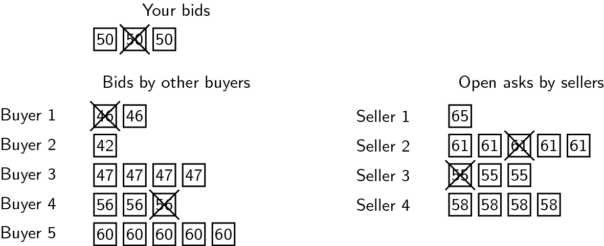
Fig. 1 Schematic representation of the screen layout for DA (buyers)
Double auction institution Figure 1 displays a graphical illustration of the interface for DA (for buyers). In DA all traders could simultaneously make offers and accept open offers by traders from the other market side. That is, there was no auctioneer or market-maker, and all offers were visible for all traders. Traders could offer any number of units
 , with
 being the remaining number of units that could be traded, at any price p by submitting an offer of the form (p, q), subject to the constraint of not incurring a net loss within a trading period.Footnote 12 At any point in time a trader could have at most one active offer. However, offers could be withdrawn or replaced by new offers at any time. A submitted offer remained active until it was withdrawn or replaced by a new offer. Further, traders could always accept active offers by the other market side. All traders could see all open offers from both buyers and sellers (see Figure 1). Offers from the own and the other market side were always shown on the left and right parts of the screen, respectively. Each offer (p, q) was represented by q boxes showing the price p with each box representing an offer to buy/sell one unit at that price (see Figure 1). Traders could accept offers from the other market side, that is buy/sell one unit at the shown price, by clicking on the corresponding box. Traded units were indicated by crossed-out boxes and remained visible until the end of the trading round. Each subject could trade up to a maximum of 6 units and the remaining number of units that could be traded at any point was shown on screen. Additionally, buyers, respectively sellers, were shown the resale values, respectively production costs, for each of the six units as well as the price of already-traded units. Subjects could leave the trading stage by pressing the “leave market stage” button, in which case any still-active offer was withdrawn. The maximum duration of a trading round at DA was 90 seconds, with the remaining time shown on screen. Alternatively, the market platform was closed if no further trade was possible (for example because all buyers had left the trading stage or all sellers were out of stock).
Our design follows the classical Multiple Unit Double Auction (MUDA) design of Plott and Gray (Reference Plott and Gray1990), with the exception that in their design only the highest-price bid and the lowest-price ask are shown (replacing previous ones), while in our design subjects observe all offers. Subjects were able to see all transactions in real-time, but no graphical representation or order book were provided.
Posted offer institution In PO buyers and sellers moved sequentially in two distinct stages. In the first stage, sellers simultaneously submitted offers of the form (p, q) proposing to sell q units at price p.Footnote 13 Each seller was only able to submit a single offer (p, q) (similarly to DA, where each trader could have at most one active offer at any point in time). Sellers were shown their production costs for all six units, but received no information about the offers made by other sellers during this stage. This first stage lasted for a maximum of 20 seconds, or, alternatively until all sellers had committed to an offer. At the end of this stage the offers made by all sellers were collected and the second stage began. In that stage, buyers moved sequentially in a randomly-determined order. When a buyer’s turn came, he observed all offers made in the first stage, as well as all units bought by previous buyers, and could buy units by clicking on still-available offers. As in the DA case, available offers were indicated by numbered boxes and already-traded units by crossed-out boxes (as in the right part of Fig. 1).Footnote 14 A buyer’s turn ended after 20 seconds or once no further units were available. The trading round ended once all buyers had had their turn, or no further units were available.
2.3 Treatments
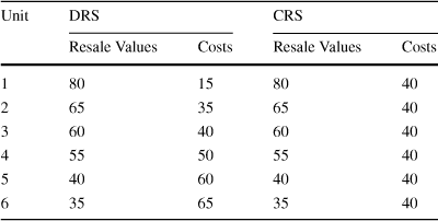
In a given round, the resale values and production costs of the traders that opted for a particular institution determined the induced supply and demand at that institution. There were two treatments, DRS and CRS, which correspond to decreasing and constant returns to scale for the supply side of the market, respectively. Specifically, the treatments differed in the resale values and production costs as given in Table 2.Footnote 15 In both treatments the demand function induced via buyers’ resale values was decreasing in the price. This was accomplished by setting decreasing resale values for each unit traded by a buyer. In treatment DRS, sellers faced increasing production costs (decreasing returns to scale), hence the induced supply function was increasing in the price. In treatment CRS, sellers faced a constant production cost instead (constant returns to scale), and as a consequence the induced supply function was flat. In each round a common shock
 was added to all these baseline resale values and production costs, so that the exact numbers varied from round to round, but induced demand and supply were unaffected.
2.4 Hypotheses
Given demand and supply, the DA typically leads to higher efficiency than the PO. Intuitively, if selection of market institutions is driven only by efficiency, over time traders should learn to coordinate on the efficient institution. However, efficiency is only concerned with overall trader surplus but not with the distribution of these gains from trade between buyers and sellers. The latter introduces a tradeoff between efficiency and profits for one market-side that could prevent coordination on the efficient institution.
In treatment DRS, the distribution of profits is “symmetric” in the sense that for prices at the market clearing level both buyers and sellers make positive profits. Consequently, in this treatment the aforementioned tradeoff is expected to be absent and convergence on the efficient institution should occur.
Hypothesis 1
In DRS, traders learn to coordinate on DA over time with PO becoming mostly inactive in the final rounds.
In contrast, treatment CRS presents exactly an “asymmetric” setting where market power is biased toward buyers in the sense that at prices at the market clearing level sellers make zero profits and buyers reap all the gains from trade. Hence, sellers have to choose between an efficient institution where their profits are (close to) zero and an inefficient institution which, due to its structure, typically leads to higher prices and seller profits. This tradeoff might hinder coordination on DA leading to slower convergence and survival of the inefficient PO institution.
Hypothesis 2
In CRS, coordination on DA is slower than in DRS with both institutions remaining active until the last round.
3 Equilibrium prices and market-clearing benchmark
In this section, we consider the theoretical benchmark where markets clear, taking as given an allocation of traders to institutions, and derive equilibrium market prices and total trader surplus, which we will use as a benchmark to measure efficiency.
Fix an institution, and consider the population of traders that has chosen to trade at that institution. This population consists of n buyers and m sellers (with
 in the experiment). Each trader can trade up to Q units (
 in the experiment) of a single homogeneous good. Denote the price of the good by
 . A typical buyer is characterized by a vector of resale values
 with
with
 where
where
 is the buyer’s resale value for the kth unit. A typical seller is characterized by a vector of production costs
 with
with
 where
where
 is the seller’s production cost for the kth unit. Assume that
 , that is, beneficial trade is possible for any
 . For a given price p, the resale values induce a (weakly) decreasing demand function given by

That is, demand is given by the largest number of units that the n buyers are willing to purchase (implicitly assuming, for simplicity, that traders are willing to trade when exactly indifferent). Specifically, if
 , k is the unique number such that
 . If
. If
 , then
 and demand is given by nQ (the capacity constraint becomes binding). If
 , the set over which the supremum is taken above is empty (so the supremum is formally
 ), and hence
 and demand is nonexistent. The induced demand function is illustrated in Fig. 2 for both treatments in the experiment, for the case where all 8 buyers are at the same institution.
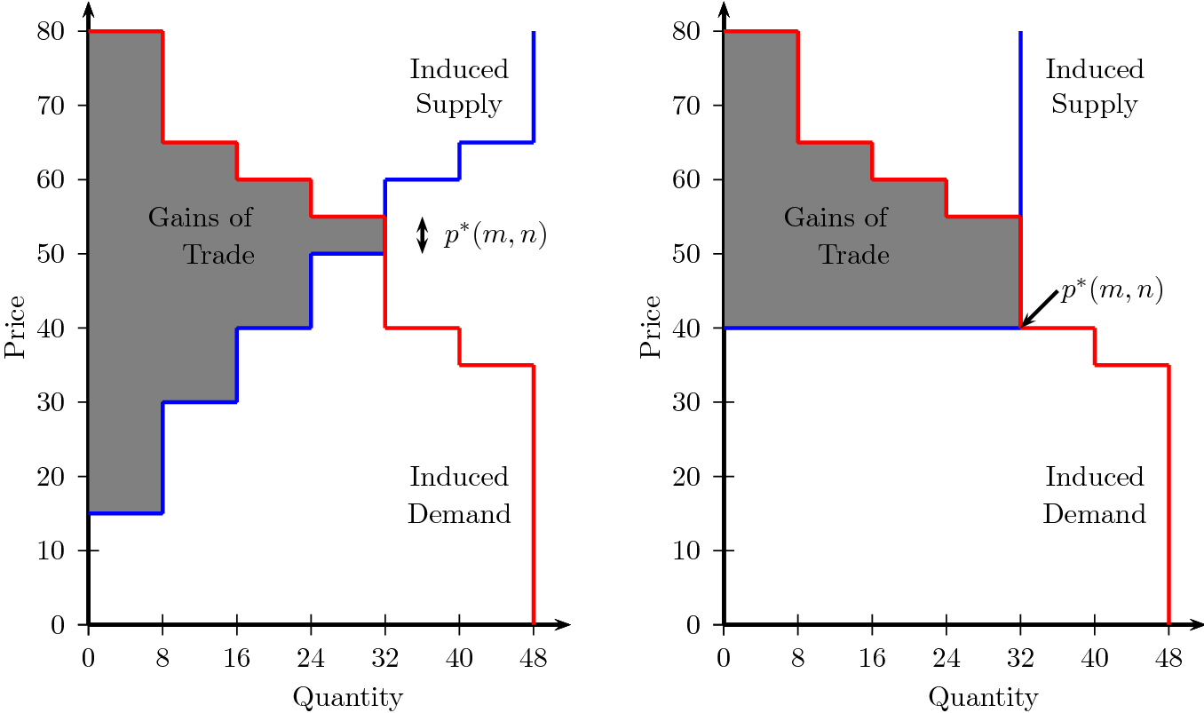
Fig. 2 Induced demand and supply functions for both treatments (DRS left, CRS right) in case of full coordination on the respective institution
Analogously, for a given price p, the production costs induce a (weakly) increasing supply function given by

That is, supply is given by the largest number of units that the m sellers are willing to sell. Specifically, if
 , k is the unique number such that
 . If
. If
 , then
 and supply is given by mQ (the capacity constraint becomes binding). If
 ,
,
 and supply is nonexistent. The induced supply function is illustrated in Fig. 2 for both treatments in the experiment, for the case where all 8 sellers are at the same institution.
In our discrete setting, demand and supply are step functions and hence equilibrium prices might correspond to an interval instead of a unique value. Let
 and
and
 . It follows that
 and
and
 . Further, note that
 , and, since
 , at least one of
 and
and
 must be finite.
The set of equilibrium prices
 is given by
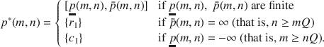
Figure 2 illustrates
 for both treatments in the experiment, for the particular case
 . Note that
 implies that
 and demand always exceeds supply, hence
 is the unique equilibrium price at which trade actually occurs. Analogously, if
 ,
,
 , supply always exceeds demand, and
 is the unique equilibrium price at which trade occurs.
In our experiment, the resale values were given, and the production costs varied across treatments (DRS and CRS). Tables B.1 and B.2 in the Online Appendix report the equilibrium price intervals for both treatments. In the analysis below, and as a first measure of the efficiency of the institution, we will report the distance from actually-realized trading prices per round to the benchmark equilibrium price intervals
 .
.
As a second measure of efficiency, we consider the largest achievable total trader surplus for a given number of buyers and sellers. Let the mQ resale values of the m buyers be
 and let the nQ costs of the sellers be
 . The maximum gains of trade are defined as the largest-possible total trader surplus, that is

Figure 2 illustrates
 for both treatments in the experiment, for the particular case
 . The values of
 for DRS and CRS are given in Tables B.3 and B.4 in the Online Appendix, respectively. In the analysis below, we will compare the actually-realized total trader surplus (defined as the sum of the differences between resale value and production cost for all actually-traded units) to
 .
.
4 Results: Market Selection
4.1 Decreasing returns
We first consider treatment DRS, where the supply side faced decreasing returns to scale (
 in 15 market observations). The top-left panel of Figure 3 shows the average number of buyers and sellers at DA for each period. We see a clear convergence toward DA over time.Footnote 16 That is, as time goes by, more and more traders of each market side choose the DA. This is confirmed in a series of linear random effects regressions on the number of buyers/sellers at DA per period, as reported in Table 3.Footnote 17 The variable RatioDA is the (lagged) buyer-seller ratio at DA. The regressions show that buyers are attracted by a low buyer-sellers ratio, but the latter has no effect on sellers’ behavior.

Fig. 3 Top: Average (over 15 markets) number of buyers/sellers at DA per period for DRS (left) and CRS (right). Bottom: Average (over 15 markets) fraction of markets where DA/PO is active per period for DRS (left) and CRS (right)
Table 3 Linear random effects regressions for DRS

|
Number of buyers at DA |
Number of sellers at DA |
|||
|---|---|---|---|---|
|
1 |
2 |
3 |
4 |
|
|
Period |
0.0734
|
0.0636
|
0.0959
|
0.0864
|
|
(0.0074) |
(0.0074) |
(0.0088) |
(0.0090) |
|
|
RatioDA |
−0.5988
|
0.1776 |
||
|
(0.1308) |
(0.1373) |
|||
|
Constant |
5.8000
|
6.5959
|
5.3580
|
5.3413
|
|
(0.3470) |
(0.2954) |
(0.3790) |
(0.3387) |
|
|
|
0.1193 |
0.1652 |
0.1663 |
0.1194 |
|
Observations |
375 |
359 |
375 |
359 |
|
Markets |
15 |
15 |
15 |
15 |


Robust standard errors in parentheses.

 ,
,

 ,
,


The bottom-left panel of Fig. 3 shows the fraction of markets where DA and PO are active over time. Across all 15 markets the DA is active in all but one period for a single market, that is, on average the DA is active 99.7% of the time. In contrast, the PO is only active 48% of the time. The average fraction of periods in which DA is active is significantly larger than the average fraction of periods in which PO is active (Wilcoxon signed-rank test, WSR:
 ,Footnote 18
 ,
,
 ). We obtain a similar result for the average number of buyers or sellers, that is, on average there are more buyers and more sellers at DA than at PO (WSR, buyers:
 ,
,
 ; sellers:
 ,
,
 ).
).
To confirm that traders increasingly coordinate on DA over time, we compare coordination at the beginning against coordination at the end of the experiment. To that end, we exclude the first period and split the remaining 24 periods in three parts of 8 periods each (see the Online Appendix for an alternative specification). We first consider the fraction of time DA or PO are active in part 1 vs. part 3. Because DA is essentially active in all periods, there is no difference for DA between parts 1 and 3 (WSR,
 ,
,
 ). On the other hand, PO is active more often in part 1 (64.2% of the time) than in part 3 (28.3%; WSR,
 ,
,
 ). A similar picture emerges when looking at the number of buyers and sellers at DA, which is significantly larger at the end of the experiment compared to the beginning (WSR, buyers:
 ,
,
 ; sellers:
 ,
,
 ).
).
4.2 Constant returns
We now consider treatment CRS (
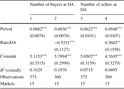
 in 15 different market observations). The top-right panel of Figure 3 illustrates the evolution of the number of buyers and sellers at DA over the course of the experiment in CRS. We again observe convergence toward DA, although it appears to be slower than in the case of DRS (see next subsection for a treatment comparison).Footnote 19 Table 4 displays a series of linear random effects regressions of the number of buyers/sellers at DA on period and shows that traders move toward DA over time.Footnote 20 Buyers are attracted by a low buyer-seller ratio, and the opposite is true for sellers.
Table 4 Linear random effects regressions for CRS
|
Number of buyers at DA |
Number of sellers at DA |
|||
|---|---|---|---|---|
|
1 |
2 |
3 |
4 |
|
|
Period |
0.0882
|
0.0836
|
0.0622
|
0.0548
|
|
(0.0078) |
(0.0078) |
(0.0101) |
(0.0107) |
|
|
RatioDA |
−0.5331
|
0.3603
|
||
|
(0.1127) |
(0.1558) |
|||
|
Constant |
5.1153
|
5.7994
|
5.0507
|
4.7695
|
|
(0.3315) |
(0.2999) |
(0.3159) |
(0.3279) |
|
|
|
0.1629 |
0.1870 |
0.0715 |
0.0495 |
|
Observations |
375 |
360 |
375 |
360 |
|
Markets |
15 |
15 |
15 |
15 |


Robust standard errors in parentheses.

 ,
,

 ,
,


The bottom-right panel of Figure 3 shows the fraction of markets in CRS where DA and PO are active over time. DA is always active, whereas PO is only active 66.4% of the time, which is significantly less often than DA (WSR:
 ,
,
 ). Buyers and sellers favor DA over PO, that is, on average there are both more buyers and more sellers at DA (WSR, buyers:
 ,
,
 ; sellers:
 ,
,
 ).
).
As in the previous treatment, we compare coordination in parts 1 (periods 2–9) and 3 (periods 18–25). We first consider the fraction of time DA or PO are active in part 1 vs part 3 of CRS. Because in CRS DA is always active in all periods, there is no difference for this platform. On the other hand, PO is active more often in part 1 (78.3% of the time) than in part 3 (59.2%; WSR,
 ,
,
 ). The analogous statement holds for the number of buyers and sellers at DA, which is significantly larger in part 1 compared to part 3 (WSR, buyers:
 ,
,
 ; sellers:
 ,
,
 ).
).
4.3 Treatment comparison
We now compare the results of treatment CRS with those of the DRS treatment. Examination of Figure 3 suggests that convergence toward coordination on DA is slower in the case of constant returns to scale. A treatment comparison shows that, indeed, there are on average more buyers and more sellers at DA in DRS than in CRS (Mann-Whitney-U test, MWU, buyers:
 ,Footnote 21
 ,
,
 ; sellers:
 ,
,
 ).Footnote 22
The differences are also reflected in the comparison between the beginning and the end of the experiment. Although there is no difference in activity for DA or PO in part 1 (MWU, DA:
 ,
,
 ; PO:
; PO:
 ,
,
 ), in part 3 PO is marginally more active in CRS than in DRS (MWU,
 ,
,
 ). Activity is, however, a somewhat coarse measure, hence we turn to the number of buyers and sellers at DA as a more fine-grained measure of convergence. With this measure, we find that already at the beginning of the experiment more buyers and sellers coordinate on DA in DRS compared to CRS (MWU; buyers,
 ,
,
 ; sellers,
 ,
,
 ). The difference subsists at the end of the experiment (buyers,
 ,
,
 ; sellers,
 ,
,
 ).
).
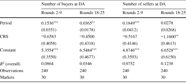
Table 5 displays the results of linear regressions comparing the number of buyers and sellers in the first and last parts of the experiment (rounds 2-9 and 18-25, respectively) across treatments. That is, the dummy CRS takes the value 1 for market observations in that treatment. We observe that the number of sellers at DA is significantly smaller for CRS market observations, but only in part 3.Footnote 23
Table 5 Regressions for comparison DRS vs CRS in first and last part
|
Number of buyers at DA |
Number of sellers at DA |
|||
|---|---|---|---|---|
|
Rounds 2-9 |
Rounds 18-25 |
Rounds 2-9 |
Rounds 18-25 |
|
|
Period |
0.1536
|
0.0365
|
0.1849
|
0.0278 |
|
(0.0351) |
(0.0178) |
(0.0412) |
(0.0268) |
|
|
CRS |
|
|
|
|
|
(0.4058) |
(0.4318) |
(0.4146) |
(0.4613) |
|
|
Constant |
5.3554
|
6.5484
|
4.8746
|
6.6528
|
|
(0.3550) |
(0.4677) |
(0.3593) |
(0.6150) |
|
|
|
0.0864 |
0.0346 |
0.0752 |
0.1238 |
|
Observations |
240 |
240 |
240 |
240 |
|
Markets |
30 |
30 |
30 |
30 |


Robust standard errors in parentheses.

 ,
,

 ,
,


5 Results: Efficiency and the Gains from Trade
The previous section has concentrated on the market selection decision and shown that traders learn to gradually coordinate on the DA platform, although convergence is stronger under decreasing returns to scale. This section examines trading decisions within each institution, and asks whether actual trade is efficient and which market side is able to reap larger shares of the gains from trade.
5.1 Trading Efficiency and Market-Clearing
We consider two dimensions of efficiency of an institution. The first is the difference between the actual price and the equilibrium price interval
 given that n buyers and m sellers are currently present at that institution. The second is the fraction of realized gains (trader surplus) relative to the maximal possible gains of trade
 .
.
Figure 4 shows the evolution of the average price at both institutions relative to the equilibrium price, for both treatments. For illustrative purposes, what is plotted is the difference
 , where p is the realized average price and
 is the equilibrium price, if the latter is unique. If
 is a proper interval, we plot the difference with the closest value in that interval.

Fig. 4 Average (over 15 markets) of the differences between average realized prices and the equilibrium price (
 , or the difference with the closest value in the interval
 ) at PO vs. DA per period
To evaluate how close realized prices were to equilibrium ones, we consider the distance, i.e. the (average across markets of the) absolute value of the average difference each period. In DRS, realized prices where closer to equilibrium in DA (average distance 2.86) than in PO (9.45; WSR,
 ,
,
 ). This is also true in CRS, although the difference is smaller. In this treatment, the average distance between realized and equilibrium prices was 7.20 for DA and 9.25 for PO (WSR,
 ,
,
 ). Comparing treatments, for DA the distance to equilibrium prices is larger in CRS than in DRS (MWU,
 ,
,
 ), whereas we find no significant difference across treatments for PO (
 ,
,
 ).
).
Figure 5 displays the evolution of the average fraction of the maximal gains of trade which were actually realized in both treatments and for both institutions. In DRS the double auction realizes on average 95.8% of the maximum possible gains of trade, whereas in PO realized gains are only 71.2%. The difference is highly significant (WSR,
 ,
,
 ). In CRS, DA realizes 98.1% of all possible gains, while in PO realized gains are only 83.5%. Again, the difference is highly significant (WSR,
 ,
,
 ). Realized gains are higher in CRS than in DRS both for DA (MWU,
 ,
,
 ) and for PO (MWU,
 ,
,
 ).
).

Fig. 5 Average (over 15 markets) realized gains (as fraction of maximal possible gains) at PO vs. DA per period
Table 2 Baseline resale values and production costs for treatments DRS and CRS
|
Unit |
DRS |
CRS |
||
|---|---|---|---|---|
|
Resale Values |
Costs |
Resale Values |
Costs |
|
|
1 |
80 |
15 |
80 |
40 |
|
2 |
65 |
35 |
65 |
40 |
|
3 |
60 |
40 |
60 |
40 |
|
4 |
55 |
50 |
55 |
40 |
|
5 |
40 |
60 |
40 |
40 |
|
6 |
35 |
65 |
35 |
40 |
In summary, we find that DA is able to realize a larger fraction of the maximal gains of trade than PO in both treatments, coming very close to the theoretical maximum. However, the difference is larger in the DRS treatment. To see this, we compare the difference in differences and find that the relative advantage of DA over PO is larger in DRS (24.0%) compared to CRS (14.6%; MWU,
 ,
,
 ).
).
5.2 The Distribution of Gains from Trade
The previous subsection has examined efficiency at the level of an institution. In this subsection, we briefly compare the gains from trade separately for buyers and sellers, which illuminates the underlying dynamics. Figure 6 displays the per capita gains from actual trade over time in both treatments and both institutions, separately for buyers and for sellers (that is, the figure plots total gains of a market side divided by the number of actually-present traders from that side, averaged across active markets). Whereas in DRS the gains from trade remain of a comparable magnitude for both market sides and for each given market institution, with sellers sightly above buyers, in CRS a large gap opens in DA, with buyers’ gains steadily rising while those from sellers decline (the average difference between per capita buyers’ and sellers’ gains is -2.0 ECUs in part 1 and 52.9 in part 3; WSR,
 ,
,
 ). This gap also exists but is smaller in the case of PO (the corresponding average difference in part 3 for PO is 21.6, which is smaller than the one of DA; WSR,
 ,
,
 ).
).

Fig. 6 Average (over active markets) gains of buyers and sellers per period
The interpretation is as follows. Over time, more traders move toward the double auction institution (Fig. 3, top-right). In this institution, provided enough sellers are present, the price should converge to market clearing, which under constant returns to scale implies zero profits for the sellers (Fig. 4, right). Convergence, however, takes time, and even more so in a setting where traders can switch away from a given institution. This means that profits remain positive for sellers even as more of them them flock to the double auction institution and the price in the latter drops. Hence, even as the price becomes relatively close to marginal cost and buyers’ are able to reap larger and larger shares of the gains from trade, the institution remains comparatively attractive for sellers. Sellers are effectively facing a tradeoff between an institution (PO) that favors them but is gradually becoming empty, and a more efficient institution (DA) where their profits might eventually vanish but remain positive within a finite horizon.
6 Results: Switching Behavior
In this section we look at individual behavior regarding market selection. In particular, we look at market switching behavior, that is, the traders’ decision whether to leave the market they are currently at and select the other market for the next period.Footnote 24 A (market) switch is a market choice where a subject selects a market for the next round that is different from the market he is currently at. A total of 19.8% of all market-choice decisions were switches, 21.1% in the case of sellers and 18.4% in the case of buyers (obviously excluding the first period).
The previous literature on experimental markets has often looked at simple behavioral rules of thumb (e.g., imitation or myopic best reply) within single markets. In particular, and following the theoretical model of Vega-Redondo (Reference Vega-Redondo1997), a series of experimental Cournot oligopoly markets examined the role of imitation in symmetric settings where one market side is summarized by an aggregate demand function and all subjects play the role of producers. Those experiments generally found evidence in favor of imitative rules when information was centered on individual actions and profits, with possible shifts toward more forward-looking rules as myopic best reply when more information on the market structure was provided (e.g., Huck et al. Reference Huck, Normann and Oechssler1999; Offerman et al. Reference Offerman, Potters and Sonnemans2002; Apesteguía et al. Reference Apesteguía, Huck and Oechssler2007, Reference Apesteguía, Huck, Oechssler and Weidenholzer2010), although results depend on the number of players, the length of the experiment, and other factors (Bosch-Domènech and Vriend Reference Bosch-Domènech and Vriend2003; Huck et al. Reference Huck, Normann and Oechssler2004; Friedman et al. Reference Friedman, Huck, Oprea and Weidenholzer2015; Oechssler et al. Reference Oechssler, Roomets and Roth2016). For instance, Huck et al. (Reference Huck, Normann and Oechssler2002) suggested that their data would be consistent with a mixture of best reply and imitation. Those experiments, however, all consider production behavior within a single market institution. The exception is Alós-Ferrer and Kirchsteiger (Reference Alós-Ferrer and Kirchsteiger2015), who conducted an experiment on platform selection where, however, actual trade followed a reduced-form approach (that is, traders did not make actual trading decisions). Alós-Ferrer and Kirchsteiger (Reference Alós-Ferrer and Kirchsteiger2015) found evidence in favor of switching behavior reflecting which institutions had the maximum observed payoffs for the trader’s market side, which can be seen as a form of imitation.
Following this literature, we hypothesized that simple rules of thumb would be able to explain switching behavior in our data.Footnote 25 We consider three behavioral rules that specify switches of a particular type depending on different (observable) market outcomes. A buyer (seller) following a Best-Price rule chooses the institution with lowest (highest) observed price in the current period, effectively chasing after the best observed price. To prevent trivial cases, the rule also prescribes to avoid institutions where no trade occurred, hence no price was realized. A buyer (seller) following a Best-Average-Price rule chooses the institution with the lowest (highest) average price in the current period, hence taking into account that a single price might not be representative of the institution (trivial cases are avoided as in Best-Price). A more forward-looking rule is to focus on the trader ratio as a predictor of future performance. In particular, in our setting, the equilibrium market price is a function of the trader ratio, and hence focusing on the latter could be seen as an attempt to predict the former, and in this sense this rule is closer to myopic best reply. A buyer following a Best-Ratio rule chooses the institution with lowest ratio of buyers to sellers in the current period (and follows the sellers if they are all at the same institution). Analogously, a seller following this rule chooses the institution with lowest ratio of sellers to buyers in the current period (and follows the buyers if they are all at the same institution).Footnote 26
The upper part of Table 6 shows the percentage of decisions that are consistent with each rule’s prescriptions, in addition to the percentage of switching decisions, separately for buyers and sellers. All three rules explain a large percentage of decisions, with the simplest one, BestPrice, explaining the most both for buyers (81.0%) and for sellers (75.1%), but with the most sophisticated, BestRatio, coming close for sellers (74.3%). As decision inertia might explain a part of the non-switching decisions, the lower part of the table shows the fraction of switches that are consistent with following each rule, separately for trader type and treatment. BestRatio explains most switches (between 73.3% and 78.6%) for both trader types and in both treatments.
Table 6 Consistent decisions and consistent switches

|
Switches |
Consistent decisions |
||||||
|---|---|---|---|---|---|---|---|
|
BestPrice |
BestAvgPrice |
BestRatio |
|||||
|
Seller |
21.1% |
75.1% |
69.4% |
74.3% |
|||
|
Buyer |
18.4% |
81.0% |
77.7% |
67.2% |
|||
|
Consistent switches |
BestPrice |
BestAvgPrice |
BestRatio |
||||
|
DRS |
CRS |
DRS |
CRS |
DRS |
CRS |
||
|
Seller |
61.9% |
62.4% |
63.6% |
65.7% |
77.1% |
78.6% |
|
|
Buyer |
59.0% |
59.6% |
62.1% |
66.5% |
76.9% |
73.3% |
|
Notes BestPrice, BestAvgPrice, BestRatio indicate that institution with best price, best average price (for own market side), or best buyer/seller ratio, respectively, was chosen. Consistent switches are switches in line with the respective rule
Given these results, we further analyze the predictive power of BestPrice and BestRatio in a series of random effects probit regressions (Tables 7 and 8). The dependent variable is switching behavior (a dummy variable taking the value 1 if there was a switch), but the regressors are continuous variables reflecting the price or ratio differences. The regression hence considers stochastic versions of the rules where a switch is more likely the larger the price difference (or ratio difference) is. The difference in the best price is coded as the difference between the currently chosen institution and the other institution for buyers and conversely for sellers. The difference in ratios is coded as the difference in buyer-seller ratios between the current institution and the other one for buyers, and the analogous difference in seller-buyer ratios for sellers. To avoid the natural (nonlinear) asymmetry of ratios (all ratios toward one side are condensed between 0 and 1, while ratios toward the other side are in principle unbounded), we consider the logarithm of the ratio. Last, to make the coefficients of the different rules comparable, we divide each of the two resulting variables by their respective empirical standard deviation.Footnote 27 We remark that price differences and log of ratios are undefined if either institution is empty in a given period and hence the regressions must exclude those observations. However, in those cases all rules would make the same prediction, thus they play no role to compare the rules (the regressions, however, underestimate the predictive power of the rules for that reason).
Table 7 Random effect probit regression on switches for buyers

|
Switch |
DRS |
CRS |
||||
|---|---|---|---|---|---|---|
|
1 |
2 |
3 |
4 |
5 |
6 |
|
|
DiffBestPrice |
0.268
|
0.266
|
0.358
|
0.365
|
||
|
(0.026) |
(0.028) |
(0.038) |
(0.041) |
|||
|
DiffLogRatio |
0.197
|
0.006 |
0.148
|
|
||
|
(0.041) |
(0.046) |
(0.035) |
(0.040) |
|||
|
Period |
|
|
|
|
|
|
|
(0.006) |
(0.006) |
(0.006) |
(0.005) |
(0.005) |
(0.005) |
|
|
Constant |
|
|
|
|
|
|
|
(0.089) |
(0.095) |
(0.091) |
(0.080) |
(0.081) |
(0.081) |
|
|
Observations |
1350 |
1406 |
1350 |
1873 |
1929 |
1873 |


Standard errors in parentheses.

 ,
,

 ,
,


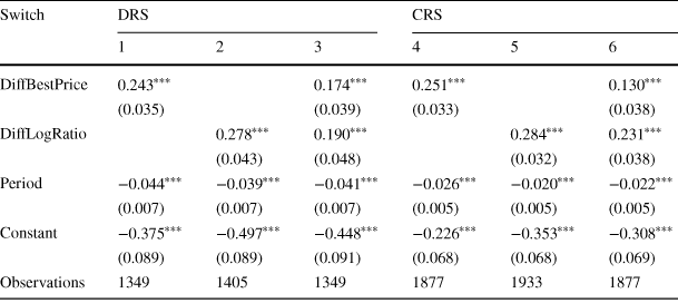
Table 8 Random effect probit regression on switches for sellers
|
Switch |
DRS |
CRS |
||||
|---|---|---|---|---|---|---|
|
1 |
2 |
3 |
4 |
5 |
6 |
|
|
DiffBestPrice |
0.243
|
0.174
|
0.251
|
0.130
|
||
|
(0.035) |
(0.039) |
(0.033) |
(0.038) |
|||
|
DiffLogRatio |
0.278
|
0.190
|
0.284
|
0.231
|
||
|
(0.043) |
(0.048) |
(0.032) |
(0.038) |
|||
|
Period |
−0.044
|
−0.039
|
−0.041
|
−0.026
|
−0.020
|
−0.022
|
|
(0.007) |
(0.007) |
(0.007) |
(0.005) |
(0.005) |
(0.005) |
|
|
Constant |
−0.375
|
−0.497
|
−0.448
|
−0.226
|
−0.353
|
−0.308
|
|
(0.089) |
(0.089) |
(0.091) |
(0.068) |
(0.068) |
(0.069) |
|
|
Observations |
1349 |
1405 |
1349 |
1877 |
1933 |
1877 |


Standard errors in parentheses.

 ,
,

 ,
,


The regressions show that both BestPrice and BestRatio are predictive of switches for both trader types if considered separately. However, when taken together, in the case of buyers only BestPrice remains significant. That is, buyer behavior appears to be usefully summarized by chasing after low prices. In contrast, for sellers both rules remain significantly predictive when considered jointly. That is, sellers seem to take into account both past high prices and favorable trader ratios, suggesting a stronger focus on forward-looking evaluations. Notably, this observation holds for both treatments, DRS and CRS.Footnote 28
The striking asymmetry in behavioral drivers between buyers and sellers is natural. In principle, in DA and under decreasing returns to scale, both trader types are treated symmetrically. However, PO is biased in favor of the sellers, and buyers are essentially passive in this latter institution. Thus, there is an institutional asymmetry which creates a tradeoff for sellers which is absent for the case of buyers. On the one hand, sellers would like to reap the high profits associated with larger prices typical of PO. On the other hand, the inefficiency of the latter institution attracts less buyers, thus leading to worse ratios for the sellers. This also holds empirically for constant returns to scale, even though in this case coordination on DA would make the sellers’ profits disappear entirely. The latter observation is less surprising in view of previous sections, since the slow speed of convergence guarantees that profits in DA, although dwindling, remain positive for sellers.
It is also interesting to note that previous empirical work on experimental markets (within a fixed institution, and with respect to trading behavior) has often suggested behavioral heterogeneity, with some subjects relying more on imitative rules and others on myopic best reply (Huck et al. Reference Huck, Normann and Oechssler1999, Reference Huck, Normann and Oechssler2002), or behavior reflecting more or less sophisticated rules depending on available information (Offerman et al. Reference Offerman, Potters and Sonnemans2002). In our markets, all traders have the same information, and they are randomly allocated to the role of buyers or sellers. Thus, the difference in behavior that we observe between buyers and sellers is causally induced by their different roles (and, specifically, the presence of an institution which treats them differently), and does not arise from cognitive or informational differences.
7 Conclusion
Most goods can be traded in different market institutions or platforms. The economics literature has intensively studied trading when the market institution is fixed, but market selection has received comparatively little attention. We study both, market selection itself, and how the presence of alternative institutions affects trade. We pit a double-auction environment, where buyers and sellers can freely trade without an auctioneer, against a posted-offers institution, where buyers are constrained to accept or reject the offers made by sellers. Although the former has been empirically shown to induce quick convergence to market clearing in isolation, the latter embodies a bias in favor of the sellers, and thus efficiency arguments suggest that traders should learn to coordinate on the double auction.
We observe coordination toward the double-auction institution, which is faster when sellers face decreasing returns to scale compared to when they are endowed with constant per-unit production costs. That is, under decreasing returns to scale, traders learn to coordinate on the efficient double auction, and the posted-offers institution becomes inactive in finitely many rounds. In contrast, under constant returns to scale, although traders tend to concentrate on the double auction, both institutions remain active until the last round. The reason is that, in the latter case, sellers try to stave off (but ultimately are not able to prevent) coordination in the double auction and the resulting convergence to market clearing prices (which would leave them with no profits).
Within institutions, and even though traders might “jump boat” at any point, trading behavior approaches equilibrium predictions in terms of prices and gains of trade. Switching behavior across institutions, however, can be explained by simple rules of thumb. Those are different across trader types: buyers seem to simply chase after low observed prices, while sellers consider both high observed prices and trader ratios. The latter might be seen as a myopic predictor of future market prices and hence reveal a more forward-looking mindset. Because traders were randomly allocated to the roles of buyers or sellers, the differences in behavior were causally induced.
Our work empirically demonstrates that efficiency alone might not suffice for a market institution to drive competing ones out of the field. Under decreasing returns to scale, fast coordination occurs because the double auction Pareto dominates the alternative, in the sense that both trader types can reap larger gains from trade. Under constant returns to scale, gains from trade are monopolized by buyers, and sellers’ earnings approach zero as prices approach the market clearing level. Thus, the distribution of gains from trade is unequal and sellers do not benefit from coordination on the efficient institution. Although, in our data, this translated into a slow-down of convergence, in general one might speculate that once profits become small enough, sellers might, in some cases and for some parameter constellations, successfully manage to turn the tide and preserve biased, inefficient institutions in the market. This might contribute to explain why multiple, possibly-inefficient institutions typically coexist for single, given goods in actual markets.
Funding
Open Access funding provided by Universität Zürich. Financial support from the German Research Foundation (DFG) through project AL-1169/5-1 is gratefully acknowledged.


 p-p∗
p-p∗ p∗(m,n)


 Open access