


1 Introduction
Many people have non-selfish preferences over the distribution of economic resources. These preferences are often synonymously called social preferences, other-regarding preferences, or distributional preferences (Fehr & Schmidt, Reference Fehr and Schmidt1999; Bolton & Ockenfels, Reference Bolton and Ockenfels2000; Charness & Rabin, Reference Charness and Rabin2002; Camerer, Reference Camerer2003; Almås et al., Reference Almås, Cappelen, Sørensen and Tungodden2010). Their existence and their specific nature are very important for economic behavior and outcomes, such as, among many others, cooperation (Boyd & Richerson, Reference Boyd and Richerson2005; Fischbacher & Gachter, Reference Fischbacher and Gachter2010), productivity (Carpenter & Seki, Reference Carpenter and Seki2011; Bandiera et al., Reference Bandiera, Barankay and Rasul2005; Dohmen & Falk, Reference Dohmen and Falk2011), political preferences (Fisman et al., Reference Fisman, Jakiela and Kariv2017; Kerschbamer & Müller, Reference Kerschbamer and Müller2020), and well-being (Becker et al., Reference Becker, Deckers, Dohmen, Falk and Kosse2012).Footnote 1 Recent studies have documented the evolution of these distributional attitudes in adolescence, from more malevolent at young ages to more benevolent when growing older. They have also stressed the large degree of individual heterogeneity of distributional preferences (Fehr et al., Reference Fehr, Glätzle-Rützler and Sutter2013; Almås et al., Reference Almås, Cappelen, Sørensen and Tungodden2010; Martinsson et al., Reference Martinsson, Nordblom, Rützler and Sutter2011; Sutter et al., Reference Sutter, Feri, Glätzle-Rützler, Kocher, Martinsson and Nordblom2018).
There are far fewer studies on the effects of the social environment and peers on distributional preferences(Charness & Kuhn, Reference Charness and Kuhn2007; Gächter et al., Reference Gächter, Nosenzo and Sefton2013; Fatas et al., Reference Fatas, Heap and Arjona2018; Bicchieri et al., Reference Bicchieri, Dimant, Gächter and Nosenzo2019). In particular, we know little about the early-life-peer influence on the emergence of distributional preferences and whether network members share distributional preferences (Hugh-Jones & Ooi, Reference Hugh-Jones and Ooi2017). To fully understand how distributional preferences are shaped in adolescence, it is important to take the close social environment and its potential influence into account. Adolescent peer networks could be important in explaining adult inter-individual heterogeneity in distributional preferences, selection into friendship/professional networks, labor market status and political views later in life, on top of potential biological determinants (Balafoutas et al., Reference Balafoutas, Kerschbamer and Sutter2012; Fisman et al., Reference Fisman, Jakiela and Kariv2017; Kocher et al., Reference Kocher, Pogrebna and Sutter2013).
Preferences could be correlated between members of social units, such as a child’s school or group of friends, beyond what is expected by the population preference distribution. Peer correlation in preferences can arise from selection into social networks whose members have similar preferences as one’s own, and through preference transmission. Besides composition, an adolescent’s position within the social network could itself be related to specific distributional preferences transmitted through various mechanisms. The potential impact of peer networks that are based on other-regarding attitudes goes beyond differential evolution of these preferences. If children are surrounded by like-minded peers, cognitive and non-cognitive abilities could also develop on different trajectories as a result of differences in cooperation and support within the network (Cunha et al., Reference Cunha, Heckman and Schennach2010; Thöni & Gächter, Reference Thöni and Gächter2015).
This paper investigates the distributional (“social”) preferences of children at primary schools in urban Tanzania and the role of peers in shaping these distributional preferences. We conduct a lab-in-the-field experiment and analyze to what extent distributional preferences of children are related to those of their peers at school, and what roles peer networks, school performance, and popularity play in explaining distributional preferences. The experiment involves choices between pairs of allocations that vary as to how much to allocate to oneself and to an anonymous passive agent (Kerschbamer, Reference Kerschbamer2015). The variation in inequality in agents’ payoffs across allocations in the choice sets allows us to classify children into four broad distributional preference types: efficiency-loving, inequality-loving, inequality-averse, and spiteful. To study the prevalence and relationships of these types in peer networks, we ask children to name and rank their three best friends. We also use survey data on background characteristics and administrative data on school grades to investigate their relationship with distributional preferences and peers.
The four distributional preference types that are used here capture a large set of potential distributional preferences under very mild assumptions see (Kerschbamer, Reference Kerschbamer2015). Efficiency-loving preferences pertain to utility functions that put emphasis on the maximum of the sum of payoffs (also called “surplus maximizing motives”). Inequality-averse preferences put disutility on inequality, whereas inequality-loving preferences put positive utility on inequality. Finally, spiteful preferences capture a disutility that is increasing in the payoffs of others (also called “competitive preferences”).
Our findings show that the majority of children exhibit choices consistent with inequality-averse (30.7%) and spiteful (42.3%) preferences. This pattern stems from a reluctance to accept disadvantageous allocations for oneself, even if they are Pareto improving. Peers’ preference types are also correlated. Even after controlling for a range of observable characteristics, we find that, if two children at the same school report a friendship link, they are 1.7% points (0.05 SD, mean = 0.33) more likely to exhibit the same preference type than if they do not. Thus, conditional on reporting a friendship link, distributional preference types of children are strongly related. This peer correlation in types is mainly driven by inequality-loving and spiteful types. Having a friend of the inequality-loving or spiteful type increases the likelihood of a child being of the same type by 6.7% points (0.2 SD) and 3.5% points (0.1 SD), respectively.
The similarity in distributional preference types in peer networks differs by gender as well, with boys driving the overall peer correlations and showing stronger correlation coefficients for spitefulness and girls sharing inequality-loving preferences.
Finally, our analysis shows that, besides network composition, the importance of the role of peers in explaining distributional preferences is linked to the position within the network. Worse relative performance in school relates positively to spiteful attitudes. The spiteful preference type is also more common when a child is central or popular within their peer networks. This suggests an importance of both social hierarchies and relative economic (human capital) position.
Our contribution in this paper is threefold. First, we investigate the role peer networks play in shaping children’s distributional preferences. Hugh-Jones and Ooi (Reference Hugh-Jones and Ooi2017) study transmission of fairness preferences in teen friendship networks and show that observing others’ choices affects adolescents’ fairness norms. We build on Hugh-Jones and Ooi (Reference Hugh-Jones and Ooi2017) and contribute to a better understanding of the evolution of preferences with age, as well as their impact on (economic) outcomes.
Second, we investigate the relationship between social hierarchies in networks and social preferences at a young age. An individual’s relative position within the social network may itself be related to distributional attitudes. We complement the view that parents’ socioeconomic status relates to the child’s social preferences (Benenson et al., Reference Benenson, Pascoe and Radmore2007; Deckers et al., Reference Deckers, Falk, Kosse, Pinger and Schildberg-Hörisch2021) by exploring the structure of the child’s own social network and its relationship to distributional preferences. If children who are disadvantaged in terms of school performance or who are less popular among peers adopt antisocial attitudes toward peers, such attitudes could be reinforced and persistently shape outcomes of future interactions. Alternatively, in line with Girard et al. (Reference Girard, Hett and Schunk2015), social structure and centrality in the social network can originate from individual preferences of children.
Third, the documentation of nuanced measures of distributional preferences at a young age in a developing country context complements a series of studies that examine distributional preferences of children in high-income contexts (Martinsson et al., Reference Martinsson, Nordblom, Rützler and Sutter2011; Fehr et al., Reference Fehr, Glätzle-Rützler and Sutter2013; Almås et al., Reference Almås, Cappelen, Sørensen and Tungodden2010; Hugh-Jones & Ooi, Reference Hugh-Jones and Ooi2017; Sutter et al., Reference Sutter, Feri, Glätzle-Rützler, Kocher, Martinsson and Nordblom2018). Distributional preferences in a setting with scarce financial resources, ethnic and religious diversity, and the absence of a welfare state, like urban Tanzania, may be of particular interest. Additionally, in an environment with high overall gender inequality, gender-specific preference formation at a young age may play an important role in explaining persistent outcome differences between males and females.Footnote 2 We therefore complement previous studies on overall and gender-specific distributional preferences of children (Benenson et al., Reference Benenson, Pascoe and Radmore2007; Almås et al., Reference Almås, Cappelen, Sørensen and Tungodden2010; Martinsson et al., Reference Martinsson, Nordblom, Rützler and Sutter2011; Fehr et al., Reference Fehr, Glätzle-Rützler and Sutter2013; Sutter et al., Reference Sutter, Feri, Glätzle-Rützler, Kocher, Martinsson and Nordblom2018; Deckers et al., Reference Deckers, Falk, Kosse, Pinger and Schildberg-Hörisch2021).Footnote 3
Combining distributional preferences and social networks might ultimately provide a workable theory of reference groups. Standard models of distributional preferences remain silent on how reference groups are formed. Our results are a first step, and they show that empirical inference on reference group (network) formation is not easy, but that it can be achieved in an environment in which there is enough control. Schools are almost perfect laboratories in this sense, allowing us not only to study the emergence of distributional preferences, but also to learn more about general aspects of network formation along distributional preferences.
The rest of the paper is structured as follows. In Sect. 2 we present our theoretical framework. Section 3 discusses the sample and data, Sect. 4 describes the experimental design in more detail, Sects. 5–6 present our results, and Sect. 7 concludes the paper.
2 Theoretical framework
In this section, we provide a theoretical mapping for our experimental design to motivate why we might observe that pairs of children who report a friendship link have a higher probability of exhibiting the same preference type than other children who attend the same school. We lay out a simple extension of the workhorse model for intergenerational transmission of preferences by Bisin and Verdier (Reference Bisin and Verdier2001), where horizontal preference adoption may differ between the general population and the close social environment. Consider a child i with distributional preference type
 , where
 , and a friend d with type
 . With some probability
 , the two children reveal the same preference type due to the distribution of types in the reference population. This likelihood depends on the fraction of that specific type in the reference population of the child, in our case, the school. With an additional probability
 , the child exhibits the same type as the friend due to reasons unrelated to the overall type distribution at the school:

with
 .
.
Our interest here is to estimate p, the correlation coefficient between the preference types of children and their friends jointly with and independently from the share of types in the reference population q(t).Footnote 4 Empirically this is achieved by sampling the peer networks of the entire reference population at the friendship dyad level. A positive p suggests that correlation in preferences between friends goes beyond q(t). Notice that it is possible that the correlation varies by preference type:
 for all t. This means that peer correlation may be preference type specific.Footnote 5 Different mechanisms may explain a peer correlation (
 ). Children may select their friends by matching on observable and unobservable characteristics, in particular their distributional preferences (ex ante similarity), i.e., they choose to form friendships with other students who have similar distributional attitudes. In a school environment, children do interact frequently and are thus able to learn about the attitudes of others. Children might also be influenced by the attitudes of their peers, such that distributional preferences could be transmitted through friends (ex post similarity). Preference transmission refers to any influence on the preference ex post to the formation of a friendship link and comprises unconscious assimilation, conscious imitation and directed socialization efforts by friends. Peer correlation in distributional preferences can therefore be decomposed into selection and preference transmission. However, disentangling transmission from selection in a sample of adolescents is empirically challenging. When participants are old enough so that one can elicit their distributional preferences meaningfully, they are likely to have grown up within the same local social and economic context, including sharing pre- or primary school classes, where transmission could take place. Generally, at this young age, it is unlikely to be possible to exploit or generate random variation in peer networks, and thus to exclude selection.Footnote 6
3 Sample and data
We elicited distributional preferences of students through a lab-in-the-field experiment at public primary schools in Dar es Salaam city, the commercial capital of Tanzania. The experiment was conducted in schools in the Ilala District at the beginning of the new school year in early 2018. In collaboration with the District Educational Office, we randomly chose 3 out of 112 schools for participation.Footnote 7 The experimental sessions took place on a single day per school during lecture hours. All present standard 6 (out of 7) students (age 12–13) participated.Footnote 8 The total sample contains 650 students, representing more than 90% of eligible students. In contrast to experiments in previous studies conducted with children after school hours, we had very little to no attrition and no selection effects into the experiment.
At the beginning of each session, students were randomly allocated to classrooms by drawing numbers. After a short survey on background characteristics and the students’ friend networks, pen-and-paper choice list experiments for distributional preferences and a money-earlier-or-later experiment were conducted.Footnote 9 The preference experiments took place in random order and were accompanied by randomly rotating teams of enumerators.Footnote 10 Students could earn money from experimental payoffs. At the end of the session, either the distributional or the time preference experiment was randomly chosen for payout, which led to guaranteed earnings between TZS 3,000 (US$1.35) and 8,000 (US$3.59), a significant amount of pocket money for these students, particularly given the low opportunity costs.Footnote 11
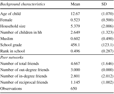
Table 1 Summary statistics
|
Background characteristics |
Mean |
SD |
|---|---|---|
|
Age of child |
12.67 |
(1.070) |
|
Female |
0.523 |
(0.500) |
|
Household size |
5.379 |
(2.006) |
|
Number of children in hh |
2.649 |
(1.323) |
|
Muslim |
0.602 |
(0.490) |
|
School grade |
458.1 |
(123.1) |
|
Rank in school |
0.496 |
(0.287) |
|
Peer networks |
||
|
Number of total friends |
4.667 |
(1.646) |
|
Number of out-degree friends |
3.000 |
(0.000) |
|
Number of in-degree friends |
2.801 |
(2.012) |
|
Number of reciprocal friends |
1.145 |
(1.002) |
|
Observations |
650 |
This table reports summary statistics of the experimental sample. School grade and rank come from the results of the national exam for grade 5, taken one month before the study. The school grade represents the grade point sum for all ten subjects: Swahili, English, mathematics, science, geography, civic education, history, art/handicraft, communication/informatics/ICT, and physical education. Rank in school is the ranking of a student of grade 6 at a given school divided by the number of grade 6 students at that school. Out-degree denotes the number of friendships reported by a student. In-degree denotes the number of friendship ties directed toward a student (i.e., reported by peers). Reciprocal friends imply that two students independently listed each other as friends
In the survey, students were asked to list and rank their three best friends within their cohort at the school. Using this information, we can construct the self-reported social networks of students. Within this network structure, various centrality measures, such as degree or eigenvector centrality, can be defined according to standard measures.Footnote 12
Table 1 presents descriptive statistics of student and network characteristics for the experimental sample. Approximately half of the participants are female, and a large proportion are Muslim, with the remaining 39.8% mostly of Christian faith. Reassuringly, the mean normalized student rank based on the overall grade by school is 0.5, which suggests we did not oversample students with good or bad grades. Social networks in the sample consist of on average of 4.7 peers, and an average student is named 2.8 times by friends. The friendship measures are bounded by the fact that only three friends per student were elicited. High standard deviations in these variables suggest that there is large heterogeneity in popularity across students.
4 Experimental design and definitions
The experimental design to elicit distributional preferences is based on Kerschbamer (Reference Kerschbamer2015).Footnote 13,Footnote 14 The exact design of the experiments and the empirical strategy were registered as a preanalysis plan prior to the fieldwork.Footnote 15 Students were asked to make ten binary choices between two payoff allocations. Each allocation consists of a payoff for the decision-maker (the active agent) and a randomly matched anonymous person (the passive agent).Footnote 16 One of the two allocations in each choice situation always gives equal payoffs to both agents (symmetric allocation). The other allocation is asymmetric, with higher payoffs for the active agent in half of the choices (advantageous block) and lower in the other half (disadvantageous block). The symmetric allocation is the same in all ten choices, while the asymmetric allocation in both blocks increases in the payoff for the decision-maker (the active agent). The changes in the asymmetric payoffs represent a change in the cost of giving to (taking from) the passive agent.
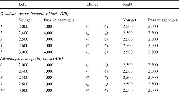
Table 2 shows the ten-item choice list design. The constant symmetric (egalitarian) allocation (right) is fixed at TZS 2,500 for both agents for the ten choices. In the five rows of the disadvantageous inequality block (DIB), the decision-maker faces lower payoffs than the passive agent (TZS 4,000) in the asymmetric allocation (left). Over the five choices, the payoff to the active agent increases monotonically from TZS 2,000 to 3,000. In the five rows of the advantageous inequality block (AIB), the decision-maker faces greater payoffs than the passive agent (TZS 1,000) in the asymmetric allocation (left). Over the five choices, the payoff to the active agent increases monotonically from TZS 2,000 to 3,000, as in the DIB.
Table 2 Choice list
|
Left |
Choice |
Right |
||||
|---|---|---|---|---|---|---|
|
Disadvantageous inequality block (DIB) |
||||||
|
You get |
Passive agent gets |
You get |
Passive agent gets |
|||
|
1 |
2,000 |
4,000 |
|
|
2,500 |
2,500 |
|
2 |
2,400 |
4,000 |
|
|
2,500 |
2,500 |
|
3 |
2,500 |
4,000 |
|
|
2,500 |
2,500 |
|
4 |
2,600 |
4,000 |
|
|
2,500 |
2,500 |
|
5 |
3,000 |
4,000 |
|
|
2,500 |
2,500 |
|
Advantageous inequality block (AIB) |
||||||
|
6 |
2,000 |
1,000 |
|
|
2,500 |
2,500 |
|
7 |
2,400 |
1,000 |
|
|
2,500 |
2,500 |
|
8 |
2,500 |
1,000 |
|
|
2,500 |
2,500 |
|
9 |
2,600 |
1,000 |
|
|
2,500 |
2,500 |
|
10 |
3,000 |
1,000 |
|
|
2,500 |
2,500 |


This table presents the choice list provided to subjects (for the actual version used in the experiment, see Figure A.2 in section 3 of the appendix). In each of 10 rows, subjects are asked to choose between two pairs of allocations (left or right). These pairs denote payoffs to the subject and to an anonymous passive agent from the same school. Payoffs are in Tanzanian shillings (TZS), US$1=TZS 2230
Since the payoff to the decision-maker on the left side increases from row to row, a rational participant should only switch from right to left and only once per block. A rational participant can also always choose left or right. The pattern of choices in the blocks determines the classification of distributional preferences. In particular, the choices reveal benevolence or malevolence toward the passive agent in the disadvantageous and advantageous domains.
Benevolence means that the decision-maker is giving up his or her own payoff to increase the passive agent’s payoff. For example, already choosing left at row 1 in the DIB reveals that the decision-maker is willing to pay at least TZS 500 to increase the passive agent’s payoff by 1,500 compared with the symmetric allocation. In the AIB, switching from left to right at row 9, or 10 also implies benevolence.
Malevolence means that the decision-maker is willing to give up his or her own payoff to decrease the passive agent’s payoff. For example, never switching implies a willingness to pay at least TZS 500 to decrease the passive agent’s payoff by TZS 1,500. Switching to the left in the DIB at row 4 or 5 reveals malevolence. In the AIB, switching to the left at row 6, 7, or 8 also implies malevolence.
The definitions of benevolence and malevolence in the two domains lump together strict and weak forms. A weakly benevolent decision-maker increases the passive agent’s payoff by choosing left at row 3 at no cost, while a weakly malevolent individual renounces doing so by choosing left at row 8.
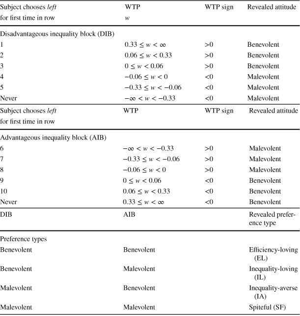
Table 3 Revealed willingness-to-pay and distributional preference types
|
Subject chooses left |
WTP |
WTP sign |
Revealed attitude |
|---|---|---|---|
|
for first time in row |
w |
||
|
Disadvantageous inequality block (DIB) |
|||
|
1 |
|
>0 |
Benevolent |
|
2 |
|
>0 |
Benevolent |
|
3 |
|
>0 |
Benevolent |
|
4 |
|
<0 |
Malevolent |
|
5 |
|
<0 |
Malevolent |
|
Never |
|
<0 |
Malevolent |


|
Subject chooses left |
WTP |
WTP sign |
Revealed attitude |
|---|---|---|---|
|
for first time in row |
|||
|
Advantageous inequality block (AIB) |
|||
|
6 |
|
>0 |
Malevolent |
|
7 |
|
>0 |
Malevolent |
|
8 |
|
>0 |
Malevolent |
|
9 |
|
<0 |
Benevolent |
|
10 |
|
<0 |
Benevolent |
|
Never |
|
<0 |
Benevolent |


|
DIB |
AIB |
Revealed preference type |
|
|---|---|---|---|
|
Preference types |
|||
|
Benevolent |
Benevolent |
Efficiency-loving (EL) |
|
|
Benevolent |
Malevolent |
Inequality-loving (IL) |
|
|
Malevolent |
Benevolent |
Inequality-averse (IA) |
|
|
Malevolent |
Malevolent |
Spiteful (SF) |
|
This table shows how a choice sequence translates into the active agent’s willingness to pay (WTP) to increase/decrease the passive agent’s payoff by TZS 1
Table 3 clarifies how a choice sequence translates into the active agent’s willingness to pay (WTP) to increase/decrease the passive agent’s payoff by TZS 1. The choice list structure of the experiment only allows us to identify WTP intervals, which is sufficient to determine the signs of the WTP. Benevolence and malevolence are used to categorize subjects into four major distributional preference types. An individual who makes benevolent choices in both domains is labeled as “efficiency-loving” (EL) –that is, the decision-maker maximizes total payoffs. A subject who chooses to switch to the asymmetric allocation early in both domains reveals a preference for inequality; thus the label “inequality-loving” is used (IL). In contrast, switching to the asymmetric allocation late or never in both domains means that we classify the individual as “inequality-averse” (IA). A subject with malevolent choices in both domains is assigned to the “spiteful” preference type (SF).
At the beginning of the experiment, the instructions of the experiment and an example choice list to illustrate the choices were read to all participants.Footnote 17 In particular, subjects were informed that the passive person was a randomly chosen participant in the same session. Subsequently, students’ remaining questions were answered personally by the team of enumerators.
It was made clear that, if a student drew the distributional preference experiment for payout at the end of the session, one of the ten items on the choice list would be randomly chosen and realized. Due to random matching of active and passive agents, apart from actively choosing allocations, each child was guaranteed to be a passive agent for some other student. The passive payoff from the randomly matched participant was added to the active payoff of the decision-maker, and this was made clear in the instructions.
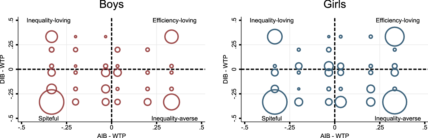
Fig. 1 Distribution of distributional preferences by gender. Note: Distributional preferences based on willingness to pay (WTP) to increase the passive agent’s payoff in disadvantageous (DIB, y-axis) and advantageous (AIB, x-axis) domains. Left: boys (293 observations). Right: girls (319 observations).
5 Results
5.1 Preference distribution and peer network characteristics
The first step of the analysis is to document the prevalence of distributional preference types in the sample. Figure 1 plots the metric willingness-to-pay measure to increase the passive agent’s payoff in the DIB (y-axis) and AIB (x-axis) and assigns preference types per quadrant. For most children, their choices can be clearly attributed to one of the four broad preference types, defined by the graphs’ quadrants. Only in the range between spiteful and inequality-averse types do some subjects show more nuanced preferences, as they reveal neutrality if advantaged and neutrality or malevolence if disadvantaged. These types are consistent with kick-down or selfish preferences (Kerschbamer, Reference Kerschbamer2015). The visualization also highlights that, while fairly balanced across the advantageous domain, choices in the disadvantageous domain are skewed toward malevolence.
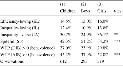
Table 4 shows that a high percentage (42.3%) of children reveal spiteful behavior in the experiment. Less than half of the subjects show either efficiency-loving (14.5%) or inequality-averse (30.7%) preferences.Footnote 18 A large share of students exhibit malevolent behavior in either the DIB (73.0%) or the AIB (54.8%), meaning that they sacrifice resources to improve their relative position. If advantaged, they choose to preserve the inequality, and, even more strongly, if disadvantaged, they decide to equalize payoffs.Footnote 19 Although Fehr et al. (Reference Fehr, Glätzle-Rützler and Sutter2013) use a somewhat different experimental design, the shares of revealed preference types from our experiment mirror almost one-to-one the distribution of 8- to 9-year-olds in their study of Austrian students. Compared with 12- to 13-year-old children in their sample, we document approximately three times higher frequencies of spitefulness and three times lower frequencies of efficiency-loving or altruistic types.
Table 4 Distribution of distributional preferences
|
(1) |
(2) |
(3) |
||
|---|---|---|---|---|
|
Children |
Boys |
Girls |
t-test |
|
|
Efficiency-loving (EL) |
14.5% |
13.0% |
16.0% |
|
|
Inequality-loving (IL) |
12.4% |
10.9% |
13.8% |
|
|
Inequality-averse (IA) |
30.7% |
24.9% |
36.1% |
mikael.lindahl@economics.gu.se |
|
Spiteful (SF) |
42.3% |
51.2% |
34.2% |
Alem et al. |
|
WTP (DIB)
|
27.0% |
23.9% |
29.8% |
|
|
WTP (AIB)
|
45.2% |
37.9% |
52.0% |
Alem et al. |
|
Observations |
612 |
293 |
319 |


Columns 1, 2 and 3 of this table show summary statistics of distributional preferences of the whole sample of children and the subsample of boys and girls. WTP denotes a subject’s willingness to pay to increase (decrease) the payoff of the passive agent in the disadvantageous (advantageous) inequality block
Distributional preferences vary significantly by gender. Girls are substantially more likely to be inequality-averse (36.1 to 24.9%) and less likely than boys to exhibit spiteful preferences (34.2 to 51.2%). This gender difference at a young age is the result of more benevolent choices of girls for both disadvantageous and advantageous allocations. In particular, when the allocation is in their favor (AIB), female students are statistically significantly more willing to sacrifice resources in order to increase the passive agent’s payoff. In fact, 23.8% more girls do so in the advantageous than in the disadvantageous domain, while for boys this difference amounts to only 14.0%. Additionally, we check if distributional preferences vary depending on whether a child lives with both biological parents, with a single parent or with none. This proxy for orphanhood, a common characteristic of children in the study context, does not correlate with the preference type; see Table A.4 in section 1 of the appendix for details.
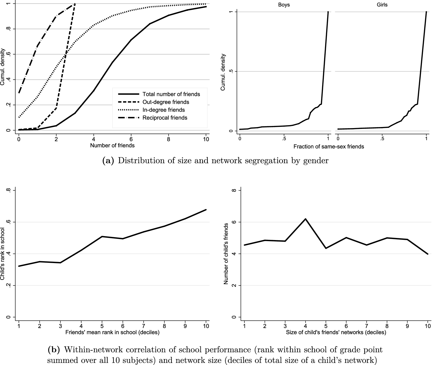
Fig. 2 Characteristics of peer networks
The peer network constructed from the three best friends of each child provides information on the quantity and the types of peers. We define “friendship” as a unilateral or bilateral link in the network. Figure 2 summarizes some of the main characteristics of these networks. By design, our network measure limits out-degree (naming a friend) to a maximum of three, which corresponds to the number of friends that we elicited via the survey. Within the observable range, the distribution does not have large tails of very unpopular or popular students (i.e., in-degree, being named as a friend). The median number of peers is only slightly lower (5) than the mean (5.6), and the standard deviation (2) is moderate. More than every third friendship is reciprocated. Not surprisingly for this age group, friendship networks are extremely segregated by the gender of students. In our sample, 77.5% of children have only same-gender friends, and only 9% have more than one peer from the opposite gender in their peer networks.
The peer networks in the sample are dense and well connected. This implies that each student could reach out to any other student via relatively few friendship connections. There are also virtually no isolated peer networks, even considering the segregation by gender. However, as we analyze and discuss further in Sect. 5.3, there are differences in popularity and centrality of children within their networks.
Despite the focus on understanding whether and why peer networks are based on distributional preferences, it is worth noticing that members of these networks can exhibit similarities in other characteristics as well. Graph (b) of Fig. 2 shows that students with high test scores also have high-performing friends (corr. 0.34
 ). Peer networks could reinforce peer correlations in school performance through cooperation and social interaction based on distributional attitudes. However, popular children do not seem to socialize more with peers who are part of large networks themselves.
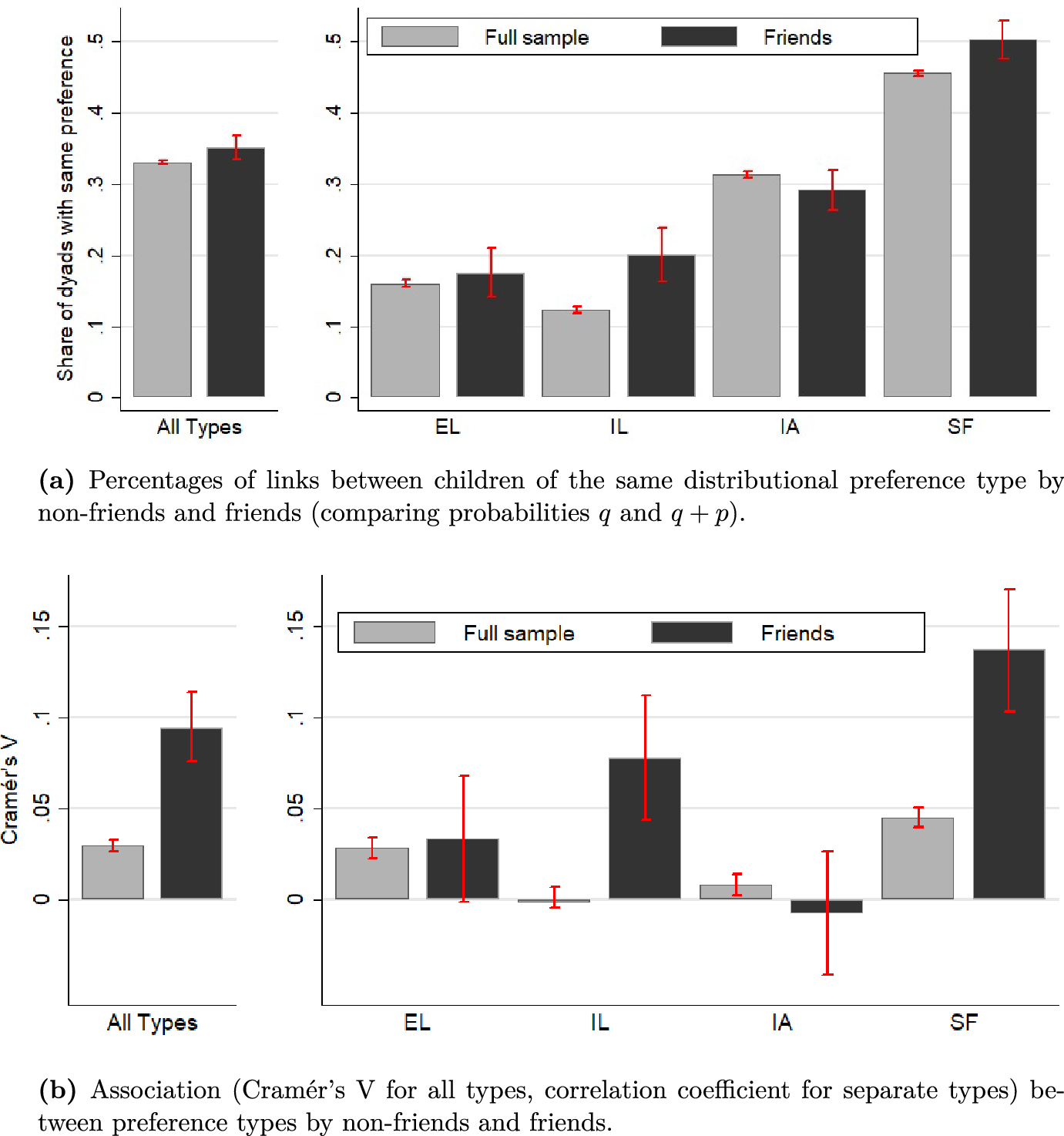
Fig. 3 Correlation of distributional preferences at the school and within peer networks.
5.2 Peer correlations in distributional preferences
We start by exploring the link between preference types in peer networks by plotting the frequency of observing pairs of children with identical preference types. Each possible pair of children at a sample school is represented by an observation (dyad) in the sample. Distinguishing between dyads of children who reported a friendship link and the full dyad sample, we can separate the probabilities p and q stated in our theoretical framework. q represents the distribution of preference types in the children’s broad social environment. In the absence of peer effects, it represents the probability that two randomly selected children exhibit the same preference type. If we observe a higher frequency of same-type dyads among those children that report a friendship, p is positive and friends are more likely to have similar preferences.
Panel (a) in Fig. 3 depicts these frequencies for the entire sample and for subsamples of specific preference types. The distribution of types in the children’s population is the major factor that explains dyads of same-type children. However, there are significant differences in the distribution of these frequencies for dyads between friends and the full sample, particularly for inequality-loving and spiteful preference types.
Panel (b) of Fig. 3 compares these frequencies to the overall preference distribution by plotting the association/correlation coefficients. For the overall relationship between the categorical types variable, we use Cramér’s V measure of association. A randomly selected pair of children at a school is more likely to exhibit the same preference type if they are friends. First, note that types between non-friends at the same school are weakly correlated (0.030), which means that q at a given school is slightly different than the overall distribution of types in our full sample of all three schools. Second, the correlation between types in dyads between friends and the full sample differs substantially and explains why we observe more same-type dyads among friends. The overall higher correlation (0.094) between types in friend-dyads is driven by significantly higher correlations for inequality-loving (0.078) and spiteful types (0.137).
Next, we take a closer look at these correlations between types for friend-dyads by controlling for observable child characteristics and uncovering some of the heterogeneity in preference peer networks using the following dyad-level specification with child i and dyad link d.

where sametype is a dummy variable equal to one if the two children in a dyad reveal the same preference type. Friendship is a dummy equal to one if one child in the dyad unilaterally reported a friendship with the other. Controls X include school fixed effects, total number of friends, school grade, age, gender, religion, same gender and same age dyads and household size. Standard errors are bootstrapped at the child level.Footnote 20 We also estimate this specification for preference type
 subsamples.
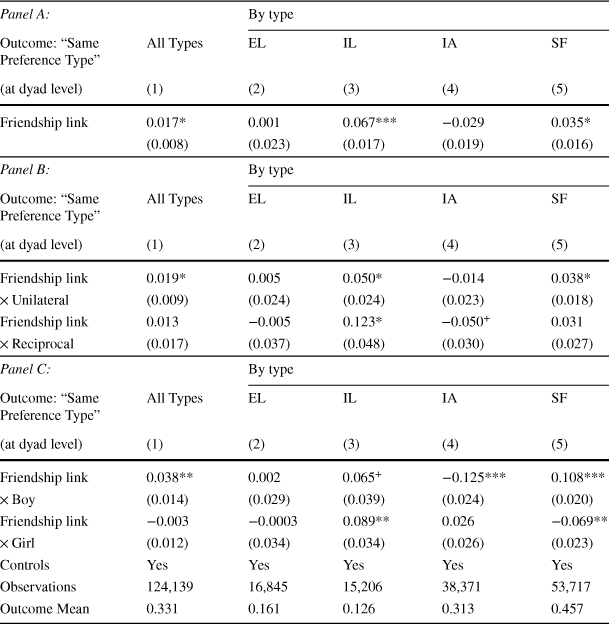
Table 5 Correlation in distributional preference types
|
Panel A: |
By type |
||||
|---|---|---|---|---|---|
|
Outcome: “Same Preference Type” |
All Types |
EL |
IL |
IA |
SF |
|
(at dyad level) |
(1) |
(2) |
(3) |
(4) |
(5) |
|
Friendship link |
0.017* |
0.001 |
0.067*** |
−0.029 |
0.035* |
|
(0.008) |
(0.023) |
(0.017) |
(0.019) |
(0.016) |
|
|
Panel B: |
By type |
||||
|---|---|---|---|---|---|
|
Outcome: “Same Preference Type” |
All Types |
EL |
IL |
IA |
SF |
|
(at dyad level) |
(1) |
(2) |
(3) |
(4) |
(5) |
|
Friendship link |
0.019* |
0.005 |
0.050* |
−0.014 |
0.038* |
|
|
(0.009) |
(0.024) |
(0.024) |
(0.023) |
(0.018) |
|
Friendship link |
0.013 |
−0.005 |
0.123* |
|
0.031 |
|
|
(0.017) |
(0.037) |
(0.048) |
(0.030) |
(0.027) |


|
Panel C: |
By type |
||||
|---|---|---|---|---|---|
|
Outcome: “Same Preference Type” |
All Types |
EL |
IL |
IA |
SF |
|
(at dyad level) |
(1) |
(2) |
(3) |
(4) |
(5) |
|
Friendship link |
0.038** |
0.002 |
|
−0.125*** |
0.108*** |
|
|
(0.014) |
(0.029) |
(0.039) |
(0.024) |
(0.020) |
|
Friendship link |
−0.003 |
−0.0003 |
0.089** |
0.026 |
−0.069** |
|
|
(0.012) |
(0.034) |
(0.034) |
(0.026) |
(0.023) |
|
Controls |
Yes |
Yes |
Yes |
Yes |
Yes |
|
Observations |
124,139 |
16,845 |
15,206 |
38,371 |
53,717 |
|
Outcome Mean |
0.331 |
0.161 |
0.126 |
0.313 |
0.457 |


This table reports marginal effects from a probit regression of a friendship link. The outcome is a binary variable equal to one if two children at a school exhibit the same preference type. Column 1 shows the marginal effect on having the same preference type. Columns 2-5 report the results for subsamples of the child’s preference type (EL = efficiency-loving, IL = inequality-loving, IA = inequality-averse, SF = spiteful). Panels B and C report correlations for unilateral and reciprocal friendship links and by the child’s gender. In all panels standard errors are bootstrapped at the child level, and controls include student’s school grade, household size, religion, age, gender, dummies for gender-matched and age-matched dyads and school fixed effects.

 , *
, *
 , **
, **
 , ***
, ***

Panel A of Table 5 shows marginal effects of a probit regression for Eq. (2). It confirms that the higher correlation between types for friends persists when school fixed effects and individual characteristics of the child are included. If two randomly selected children report a friendship, the likelihood of revealing the same preference type (mean=0.331) increases by 1.7 percentage points. Inequality-loving (mean=0.126) and spiteful types (mean=0.457) account for a large share of this relationship. In a regression using a subsample of friends with these types, the likelihood increases by 6.7% points and 3.5% points, respectively.Footnote 21 Overall, the evidence suggests that peer correlations are large for malevolent but not for benevolent choices, and thus for preference types, in both domains of our experiment. Even though children reported their three best friends, peer networks at the school may in fact be larger. This means that our measure of peer networks is truncated at out-degree three (naming three friends). As unrecorded friendships are by design lower ranked than the recorded links, our reported coefficients could be interpreted as close-friends preference correlations.
Panel B of Table 5 shows that the peer correlations in types among friends remain fairly constant when the directed nature of the network is taken into account. Whether a child names a friend or is named by another child (unilateral link) or both (reciprocal) makes little difference for preference type relations. Looking at the estimates for subsamples by distributional preference types, we observe that girls are slightly more likely to share reciprocal friendships, and therefore the correlations are slightly higher for the inequality-loving type, which is more prevalent in female students.Footnote 22
With distinct preference distributions for boys and girls, as well as relatively segregated peer networks, one could think that peer correlations are gender specific. In panel C of Table 5, we therefore introduce heterogeneity by gender of children. Overall, the estimates for peer correlations in distributional preferences are entirely driven by boys, with a statistically significant difference at 0.1%. However, when differentiating between preference types, network results for spiteful types are driven by boys, with a marginal effect of 11% points (p-value<0.001), while girls show higher correlations in inequality-loving types (9.0% points; p-value=0.009). It is noteworthy that we control for same gender dyads, because social networks in general and preference distributions are segregated by gender. We do not want to speculate on the origins of the gender differences, because we had no ex ante expectation, and there is no economic theory that gives guidance for what we observe.
As mentioned in the theoretical section, the correlation p can be due to both transmission and selection effects, and it is very difficult to empirically disentangle the two channels. In Sect. 5 of the appendix, we discuss these issues further, including using our data to illustrate a few possible approaches on how to disentangle these channels.
Finally, we want to comment on the average effect size of friendship in our preferred specification, 1.7% points on average and significantly higher for certain types. Given the lack of comparable evidence in the experimental literature, there is no benchmark for the size of the effect. What we can do is compare the effect size of friendship regarding distributional preferences with effect sizes from observable characteristics among our control variables. The average effect size of friendship regarding distributional preferences is slightly larger than the effect size of being a Muslim (compared to being a Christian).
5.3 Relative school performance and popularity
Besides providing a reference unit in which distributional preferences are formed, changed, or reinforced, peer networks may also have an indirect influence by referencing an individual’s economic or social position. Bolton and Ockenfels (Reference Bolton and Ockenfels2000) argue that the aggregate relative position of the decision-maker matters for equity concerns and reciprocity. Charness and Rabin (Reference Charness and Rabin2002) explore Rawlsian preferences and find that individuals tend to increase the payoffs of worse-off agents but behave locally in a competitive manner. Fisman et al. (Reference Fisman, Jakiela and Kariv2017) show that distributional preferences vary across the income distribution. In this section, we use detailed data on friend networks and administrative information on test scores and explore whether distributional preferences are related to an individual’s position in school performance and popularity. These two outcomes are presumably important for the individual’s position within the networks.Footnote 23
Relative position in school performance is measured by the rank in standard 6 of a specific school.Footnote 24 Within the social network, we use a continuous variable of the mean rank difference to friends to capture the relative standing in performance of the child. Popularity is assessed by measures of centrality widely used in network analysis. The simplest one, in-degree centrality, denotes the number of incoming friendships, meaning that it counts the number of times that other students have named a child as their friend. The Katz-Bonacich (KB) centrality measure additionally captures aspects of popularity that goes beyond the direct friends. It counts all the shortest paths to reach any other friend node in the close and extended social network, while discounting those connections farther away from the child. Finally, the eigenvector (EV) centrality, as an extension of degree centrality, treats connections to friends differentially by their respective importance in the network.Footnote 25
Empirically, the relationship between relative position or popularity and distributional preferences is estimated using the following binary probit specification at the student/individual level:

where
 is a dummy variable for preference types
 and position is a variable capturing relative position or popularity of individual i measured by rank, rank difference, indegree, EV-centrality, and KB-centrality respectively. To correct the standard errors for correlation at the school level, we estimate clustered standard errors and clustered wild bootstrap standard errors with the Webb distribution (Webb, Reference Webb2014; Cameron & Miller, Reference Cameron and Miller2015). The latter corrects for bias due to the low number of clusters (three schools). A positive marginal effect on the variables captured in position would suggest that students who rank higher in school performance or are central figures in adolescent peer networks reveal distinct distributional preferences.
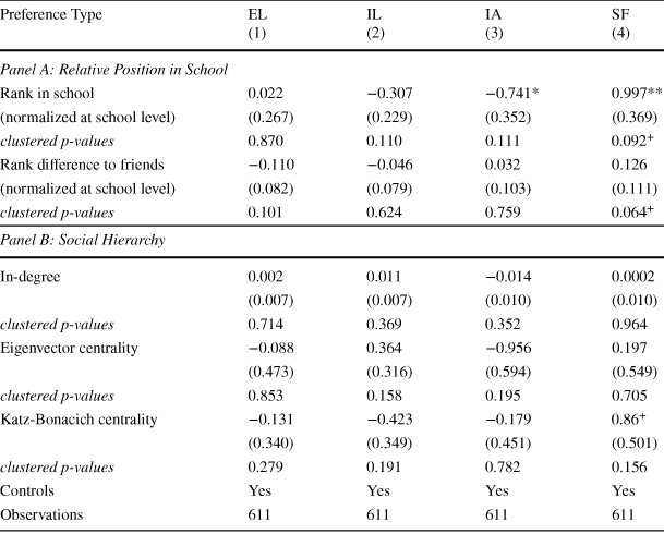
Panel A of Table 6 shows that the relative position of students in terms of educational outcomes is strongly correlated with a spiteful preference type. Note that the specification controls for the numeric school grade and identifies the relationship relatively locally. Taking the estimates at face value, this implies that, of two students who ranked one standard deviation (SD=0.29) apart, the lower-ranked student is about 29% points more likely to have spiteful preferences (p-value=0.092). On average, ranking one standard deviation lower than one’s peers increases this likelihood by 3.6% points (p-value=0.064). Relative school performance is not correlated with efficiency- and inequality-loving as well as inequality-averse types in a statistically significant manner.Footnote 26
Although intuitive, the estimates do not prove a causal relationship between relative position and spiteful distributional preferences because of potential reverse causality. Students may perform worse than their peers because of their distributional preferences or observable or unobservable confounders. We rely on survey information to tentatively argue against these alternative explanations (see Table A.2 in section 1 of the appendix). To the extent that malevolent social preferences hinder a student’s success at school, we do not find spiteful types less popular among other students or show lower self-reported frequency of studying or doing homework with friends. Concerning observable confounders, such as the social and financial status of the child’s family, the potential proxies we control for, such as household size and religion, are not correlated with spiteful preference types.
Table 6 Distributional preference and relative position (EL, IL, IA, SF)
|
Preference Type |
EL (1) |
IL (2) |
IA (3) |
SF (4) |
|---|---|---|---|---|
|
Panel A: Relative Position in School |
||||
|
Rank in school |
0.022 |
−0.307 |
−0.741* |
0.997** |
|
(normalized at school level) |
(0.267) |
(0.229) |
(0.352) |
(0.369) |
|
clustered p-values |
0.870 |
0.110 |
0.111 |
|
|
Rank difference to friends |
−0.110 |
−0.046 |
0.032 |
0.126 |
|
(normalized at school level) |
(0.082) |
(0.079) |
(0.103) |
(0.111) |
|
clustered p-values |
0.101 |
0.624 |
0.759 |
|


|
Panel B: Social Hierarchy |
||||
|---|---|---|---|---|
|
In-degree |
0.002 |
0.011 |
−0.014 |
0.0002 |
|
(0.007) |
(0.007) |
(0.010) |
(0.010) |
|
|
clustered p-values |
0.714 |
0.369 |
0.352 |
0.964 |
|
Eigenvector centrality |
−0.088 |
0.364 |
−0.956 |
0.197 |
|
(0.473) |
(0.316) |
(0.594) |
(0.549) |
|
|
clustered p-values |
0.853 |
0.158 |
0.195 |
0.705 |
|
Katz-Bonacich centrality |
−0.131 |
−0.423 |
−0.179 |
|
|
(0.340) |
(0.349) |
(0.451) |
(0.501) |
|
|
clustered p-values |
0.279 |
0.191 |
0.782 |
0.156 |
|
Controls |
Yes |
Yes |
Yes |
Yes |
|
Observations |
611 |
611 |
611 |
611 |

Columns 1–4 of this table report marginal effects from probit regressions of preference types regressed on a student’s relative position (panel A) and social hierarchy (panel B). The outcome variable is a binary variable that determines whether a student is of a specific distributional preference type (EL = efficiency-loving, IL = inequality-loving, IA = inequality-averse, SF = spiteful). Standard errors are robust, and clustered p-values reflect standard errors clustered at school level (3), computed via wild bootstrap using the Webb distribution. Controls include total size of social network, student’s
school grade, household size, religion, age, gender, and school fixed effects.

 , *
, *
 , **
, **
 , ***
, ***

Figure 4 depicts the social networks in one of the sample schools. It shows, on the one hand, that preference types appear in clusters, and, on the other hand, that spiteful types (green) are dominant in popularity, represented by size. Zooming in on this malevolent type, a central cluster located around several popular influencers emerges. This pattern is supported weakly by panel B in Table 6, which shows that all measures for centrality and popularity are related positively, although not significantly, to the likelihood of being a spiteful type. This correlation is robust to controlling for the total number of friends and therefore is not merely a reflection of large numbers of this preference type. A look at the relationship between popularity and choices in the DIB and AIB domains reveals that the correlation operates mainly through malevolence, when the asymmetric allocation is advantageous for the decision-making child. This suggests that these students are likely to prefer establishing hierarchies in the school environment that are favorable to them.
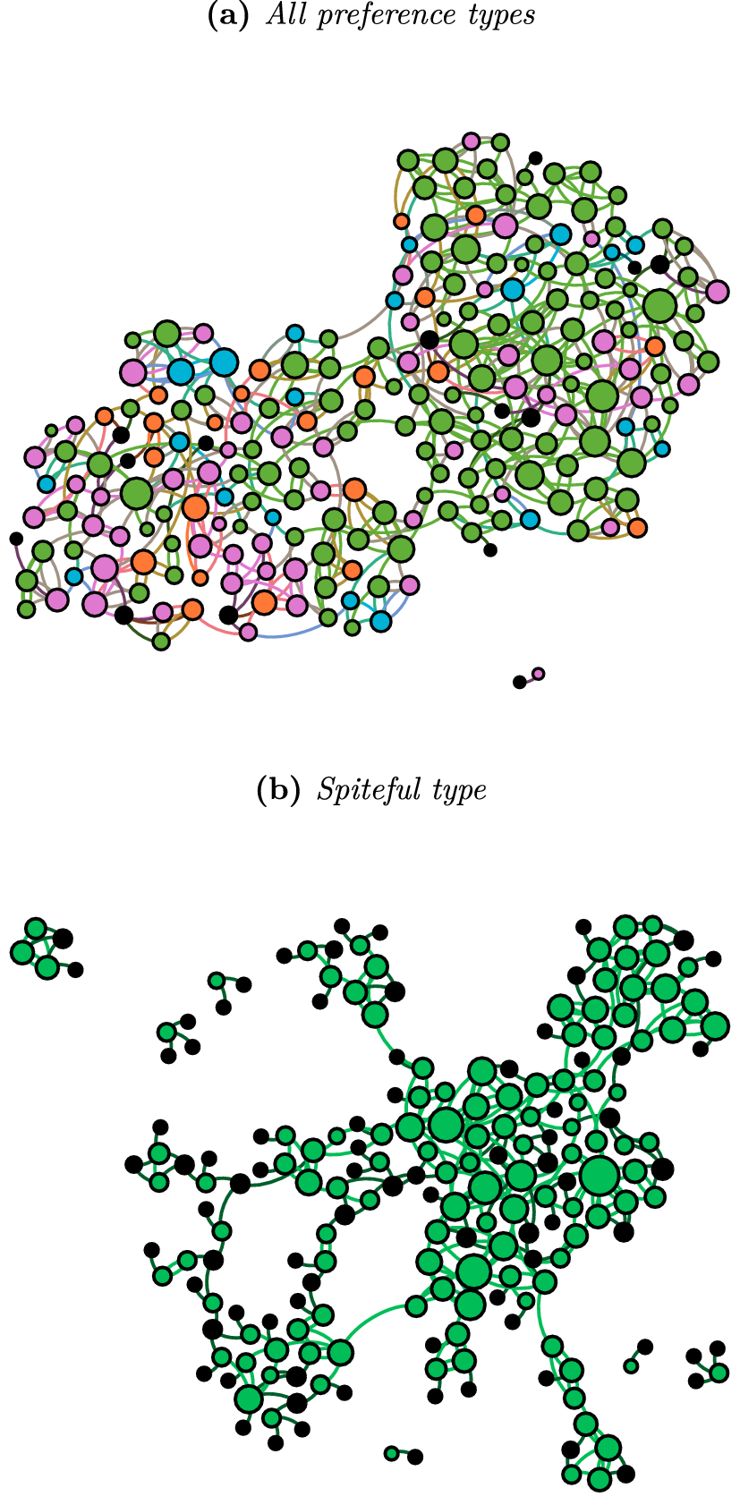
Fig. 4 Degree centrality and preference types (Maarifa Primary School). Notes: Efficiency-loving = blue, inequality-loving = orange, inequality-averse = pink, spiteful = green. Black circles in Fig. 4, panel A, denote individuals with missing preference measures; in Fig. 4, panel B, they denote all non-spiteful preference types. Figure 4, panel A, depicts all standard-6 students in the school, with colors and size denoting preference types and degree centrality. Figure 4, panel B, displays the network for children of the spiteful type
The distinction between benevolence in the DIB and AIB domains can also help explain why low ranks in outcomes and popularity show different correlations to distributional preference types. Children who are disadvantaged in terms of school grades may take the situation as exogenous-that is, not affected by their distributional attitudes towards peers-and tackle the disadvantage through malevolent choices in the DIB domain. Unpopular children may consider their social position malleable and signal benevolent behavior.
6 Additional results
While the main focus of this paper is to study the role of the close social environment of peers in understanding distributional preferences of children, our study additionally represents the first attempt to experimentally elicit these attitudes with the given method in a developing country context. Not surprisingly, we find that the country context also matters for other-regarding preferences in adolescence. As mentioned earlier, the shares of revealed preference types in our sample of 12- to 13-year-old Tanzanian children resemble the distribution of 8- to 9-year-olds in the sample of Austrian students studied by Fehr et al. (Reference Fehr, Glätzle-Rützler and Sutter2013), who also use simple allocation experiments; see footnote 3 for details. The gender gap in children’s distributional preferences is identical to the shares of preference types among 8- to 9-year-olds in that study. Thus, it appears that a 2- to 3-year delay exists in the evolution of distributional preferences, though individuals could be on different paths altogether. Interestingly, this delay corresponds to the deficits in human capital formation in Sub-Saharan Africa compared with developed countries. Bold et al. (Reference Bold, Filmer, Molina and Svensson2018) find that, after 3.5 years of school, primary schoolchildren in Kenya and Mozambique have gathered knowledge of only 1.5 years of effective learning. If economic underdevelopment is related to a low rate and slow formation of benevolent other-regarding preferences, cooperation and growth could be further affected negatively-a hypothesis, which, we believe is important to test in future research.
It is worth mentioning that the broad and close social environment may interact in determining preference formation at a young age. For example, peer networks in low-income, poverty-prone contexts could have stronger influences on economic behavior, given their role for providing crucial insurance and support in the context of a lack of efficient formal institutions, even at a young age.
This potential preference gap between low- and high-income contexts seems to persist over time. Results for comparable adults sampled in our low-income setting also differ significantly from distribution of types in developed countries (see Figure A.1 in section 2 of the appendix for the distribution of preferences in the adult sample). For example, a study in Austria by Balafoutas et al. (Reference Balafoutas, Kerschbamer, Kocher and Sutter2014), using the same design as our study, shows up to twice as many efficiency-loving types and a significantly lower occurrence of inequality-averse attitudes among adults. In fact, the distribution of adult preference types in our sample is strikingly close to the findings of Fehr et al. (Reference Fehr, Glätzle-Rützler and Sutter2013) for 14- to 17-year-old high school students in a high-income setting. We believe that this observation warrants future research as well.
7 Conclusion
Previous studies in economics have documented that distributional preferences are important in explaining a number of economic decisions in the context of fostering cooperation, increasing productivity, and improving political outcomes. How does peer influence in early life shape distributional preferences? In this paper, we attempt to shed light on this research question using a lab-in-the-field experiment. We recruited a sample of adolescents (aged 12–13) and let them make ten binary choices between two payoff allocations between the decision-maker (the active agent) and a randomly matched anonymous person from the same sample (the passive agent). We then use these allocation patterns to categorize children into efficiency-loving, inequality-loving, inequality-averse, and spiteful types. We also collect detailed information on friendship networks and investigate the relationship between distributional preferences of children and their peers.
Results suggest that a large percentage of children exhibit spiteful behavior (42.3%) or equality-oriented (30.7%) preferences. This means that a large share of students reveals malevolent behavior in their allocation decisions, i.e., they sacrifice resources to improve their relative position. If advantaged, they choose to maintain the inequality; even more strongly, if disadvantaged, they opt to equalize payoffs. There is also a clear difference between boys and girls in distributional preferences. Girls tend to be more strongly inequality-averse than boys and less likely to reveal spiteful preferences.
The detailed friendship network data we collected allows us to uncover a significant correlation in distributional preferences within the peer networks. In particular, pairs of children linked by self-reported friendship are more likely to reveal the same preference type. Conditional on a friendship link, children are alike with respect to malevolent behavior toward others, especially in disadvantageous situations (inequality-loving and spiteful types). Furthermore, the relative position within a network is related to preference types to a smaller extent than the network composition.
We believe that our study offers several novel and relevant insights on distributional preferences of adolescents and their peers. First, it provides a structured view on the role of social networks in shaping adolescents’ distributional preferences. We show that distributional preference types are assorted along friendship ties, at least for some types. Second, our study can be considered as a relevant starting point to study the emergence of reference groups that are at the heart of models of social preferences, but have not been endogenized in these models so far. Third, we show that there is a potential relationship between distributional preferences and one of the most important outcomes at a young age, school performance.
Given the importance of distributional preferences for many aspects of life, we regard it as an interesting task for future research to explore how early social preference networks shape group outcomes later in life. Our findings also speak to the potential importance of exposing children to attitudes that differ from the prevalent views of their close social environment. Children in a weak relative position or in a peer network based on malevolent preferences may not evolve with age, or at least not as quickly as others, towards exhibiting more benevolent other-regarding attitudes. Tracking or reshuffling of classes at school may be a policy that can induce exposure to other attitudes, while simultaneously changing relative positions within the social environment.
Supplementary information
The online version contains supplementary material available at (https://doi.org/10.1007/s10683-022-09775-6).
Funding
Open access funding provided by University of Gothenburg.


 Open access