


1 Introduction
Real-life decisions made under uncertainty nearly always involve ambiguity, as the probability distribution of future outcomes is not precisely known (Keynes, Reference Keynes1921; Knight, Reference Knight1921). Most people are ambiguity averse, meaning that they prefer to make decisions with known probabilities (risk) rather than with unknown probabilities (ambiguity), a fact that the subjective expected utility model cannot explain (Ellsberg, Reference Ellsberg1961). Models that accommodate ambiguity aversion were first developed in the late 1980s by Gilboa and Schmeidler (Reference Gilboa and Schmeidler1989), and extensive empirical studies on ambiguity have since been conducted (Trautmann & van de Kuilen Reference Trautmann, van de Kuilen, Keren and Wu2015). These show that people’s choices not only reveal ambiguity aversion, common for likely gains, but also ambiguity seeking for unlikely gains and for losses, similar to the four-fold pattern of risk attitudes proposed by Tversky and Kahneman (Reference Tversky and Kahneman1992).
One limitation of the available evidence on ambiguity attitudes is that these have mostly been measured with artificial events such as Ellsberg urns, rather than sources of ambiguity that decision makers face in real life. Artificial events are convenient because they can be designed to minimize the influence of people’s subjective beliefs.Footnote 1 Yet, as suggested by l’Haridon et al. (Reference I’Haridon, Vieider, Aycinena, Bandur, Belianin, Cingl, Kothiyal and Martinsson2018), the use of such artificial events may also make the experimental tasks less relevant for subjects and more difficult to understand. Recently, Baillon et al. (Reference Baillon, Huang, Selim and Wakker2018b) developed a novel method to measure ambiguity for naturally occurring sources that controls for unknown probability beliefs and risk preferences. This new method has been applied in laboratory experiments (Baillon et al., Reference Baillon, Huang, Selim and Wakker2018b; Li et al., Reference Li, Turmunkh and Wakker2019), and in the field with high school students (Li, Reference Li2017).Footnote 2
Our paper’s contribution is to measure ambiguity attitudes for relevant real-world sources in a large set of real-world investors. In particular, households often confront financial decision problems such as saving, investment, and insurance, where the probability distribution of future outcomes is not precisely known. Our objective is to measure ambiguity attitudes toward return distributions that people typically face when making such investment choices. We field a purpose-built survey module to elicit ambiguity attitudes in a representative sample of about 300 Dutch investors who participated in the annual De Nederlandse Bank (DNB) Household Survey (DHS), using the method of Baillon et al. (Reference Baillon, Huang, Selim and Wakker2018b). At the individual level, we estimate both preferences toward ambiguity and perceived levels of ambiguity about four investments: a familiar individual stock, the local stock market index, a foreign stock market index, and the crypto-currency Bitcoin. We focus on investments, as there is a large theoretical literature in finance on the implications of ambiguity.
To assess the reliability of the ambiguity attitude measures for natural sources in the field, we first conduct an econometric analysis with panel models. Correlations between repeated measures of ambiguity aversion prove to be moderate to high, in the 0.6 to 0.8 range. Individual characteristics also display significant and plausible correlations with ambiguity attitudes, and these explain 23% of the variation in ambiguity aversion. This is an improvement over previous studies that used artificial urn experiments to measure ambiguity, where individual characteristics explained only up to 3% (see Dimmock et al., Reference Dimmock, Kouwenberg, Mitchell and Peijnenburg2015; l’Haridon et al., Reference I’Haridon, Vieider, Aycinena, Bandur, Belianin, Cingl, Kothiyal and Martinsson2018). Second, our research using real-world sources confirms that ambiguity aversion is not universal.Footnote 3 We show that about 60% of the investors, on average, are ambiguity averse toward the four investments, but a sizeable fraction (40%) is ambiguity seeking or neutral.
Previous studies have shown that ambiguity attitudes have an important second component called a-insensitivity, which refers to the tendency to treat all ambiguous events as if they are 50/50% (Abdellaoui et al., Reference Abdellaoui, Baillon, Placido and Wakker2011; Fox et al., Reference Fox, Rogers and Tversky1996; Tversky & Fox, Reference Tversky and Fox1995). For unlikely events, such as new ventures that offer a large payoff with a small unknown probability, a-insensitivity implies ambiguity seeking behavior. Our results confirm that the large majority of investors displays a-insensitivity toward real-world investments, at relatively high levels on average. In the multiple prior model of Chateauneuf et al. (Reference Chateauneuf, Eichberger and Grant2007), a-insensitivity can also be interpreted as a measure of the level of perceived ambiguity. Seen this way, our results suggest that most retail investors perceive relatively high ambiguity about the probabilities of future investment returns, most likely due to limited financial sophistication as documented in the household finance literature (Gomes et al., Reference Gomes, Haliassos and Ramadorai2021). Nonetheless, a-insensitivity (perceived ambiguity) is lower for the familiar stock, and lower among investors with higher financial literacy and better education.
Our data also allow us to test whether ambiguity aversion and perceived ambiguity vary with the decision maker and the source of ambiguity. Popular theoretical formulations of ambiguity such as the smooth model (Klibanoff et al., Reference Klibanoff, Marinacci and Mukerji2005) and the alpha-MaxMin model (Ghirardato et al., Reference Ghirardato, Maccheroni and Marinacci2004) assume that ambiguity aversion is subject-dependent but constant between sources, while perceived ambiguity is both source- and subject-dependent. These key assumptions in theoretical models have, thus far, not been based on empirical evidence. We show that ambiguity aversion toward the four investments we examine is strongly related and mostly driven by one underlying variable. This implies that, if an investor has relatively high ambiguity aversion toward one specific financial asset (e.g., a stock market index), he also tends to display high ambiguity aversion toward other investments. In contrast, we find that investors’ perceived levels of ambiguity differ substantially between assets and cannot be summarized by a single measure. Accordingly, the same investor may perceive low ambiguity about a familiar stock and high ambiguity about Bitcoin.
Finally, we test whether the new ambiguity attitude measures relate to the investors’ actual investment choices. We find that investors who perceive less ambiguity about a particular financial asset are more likely to invest in it. Further, investors with higher ambiguity aversion are less likely to invest in Bitcoin. Previous studies have measured ambiguity attitudes with Ellsberg urns to avoid issues with subjective beliefs and then related these measures to portfolio choices (Dimmock et al., Reference Dimmock, Kouwenberg and Wakker2016a, Reference Dimmock, Kouwenberg, Mitchell and Peijnenburg2016b; Bianchi & Tallon, Reference Bianchi and Tallon2019; and Kostopoulos et al., Reference Kostopoulos, Meyer and Uhr2019). Our paper is the first to confirm such a link using measures of non-artificial ambiguity directly relevant for the investments.
We contribute to the empirical literature on ambiguity by measuring ambiguity attitudes toward economically relevant sources in a large sample of investors.Footnote 4 We analyze the reliability of the new elicitation method of Baillon et al. (Reference Baillon, Huang, Selim and Wakker2018b) when it is used in a survey of the general population, and we validate the measures by testing the link with actual household investments. Compared to earlier large-sample ambiguity studies using artificial events (Dimmock et al., Reference Dimmock, Kouwenberg, Mitchell and Peijnenburg2015; l’Haridon et al., Reference I’Haridon, Vieider, Aycinena, Bandur, Belianin, Cingl, Kothiyal and Martinsson2018), we find that, when using real-world sources, measurement reliability is higher and individual characteristics explain a larger proportion of the heterogeneity in ambiguity aversion.
In addition, we add to the literature on natural sources of ambiguity.Footnote 5 Fox et al. (Reference Fox, Rogers and Tversky1996) already found that even professional option traders displayed high a-insensitivity toward familiar stock return distributions. Kilka and Weber (Reference Kilka and Weber2001) showed that German students were more ambiguity averse and insensitive about a foreign stock compared to a domestic stock, displaying home bias. We can now confirm these results in a large field study of retail investors, using the latest methodology that controls for both unknown beliefs and risk preferences. In addition, our research adds to the literature on portfolio choice under ambiguity (e.g., Uppal & Wang, Reference Uppal and Wang2003; Boyle et al., Reference Boyle, Garlappi, Uppal and Wang2012; and Peijnenburg, Reference Peijnenburg2018), providing empirical evidence on how to model the ambiguity attitudes of households investing in financial markets.
2 Data and elicitation methods
2.1 Dutch household panel
We fielded a purpose-built module to measure ambiguity and risk attitudes in the CentERpanel, a representative household survey of about 2,000 respondents conducted by CentERdata at Tilburg University in the Netherlands. The survey is computer-based and subjects can participate from their homes. To limit selection bias, households lacking internet access at the recruiting stage were provided with a set-top box for their television sets (and with a TV if they had none). Each year, the DNB Household Survey (DHS) is fielded in the panel to obtain detailed information about the members’ income, assets, and liabilities.Footnote 6 We merged the DHS data with results from our survey module on ambiguity and risk attitudes. The CentERpanel is representative of the Dutch population and the DHS has previously been used to provide insight into household financial decisions (e.g., Guiso et al., Reference Guiso, Sapienza and Zingales2008; van Rooij et al., Reference van Rooij, Lusardi and Alessie2011; and von Gaudecker, Reference von Gaudecker2015).
As the panel is nationally representative, it includes a large number of people who do not invest in financial markets: about 85% of the panel members as of December 2016. Ambiguity about all investments is likely to be high in this group, without much meaningful variation between sources. To better utilize resources, our questionnaire was targeted at the 15% of DHS respondents who invested in financial assets, defined to include mutual funds (about 68% of the investors), individual company stocks (45%), bonds (11%), or options (2.5%).Footnote 7 Our survey module was fielded from 27 April-14 May 2018, yielding 295 complete and valid responses.Footnote 8 Our survey was also given to a random sample of non-investors from the general population, with 230 complete responses. The non-investor sample allows us to compare the ambiguity attitudes of investors and non-investors, which we do in Sect. 5.4. For our main results, we focus only on investors, as our goal is to assess ambiguity attitudes of investors in financial markets and to validate our measures by confirming that ambiguity attitudes are associated with investment decisions.
Summary statistics on the investor sample appear in Appendix Table 1. Education is an ordinal variable ranging from 1 to 6, where 1 indicates primary education and 6 indicates a university degree. Household Income averages €3193 per month. Household Financial Wealth consists of the sum of all current accounts, savings accounts, term deposits, cash value of insurance policies, bonds, mutual funds, stocks, options, and other financial assets such as loans to friends or family, all reported as of 31 December 2017. Mean (median) wealth was €142,357 (€84,489). We also have measures for Age, Female, Single, Number of Children living at home, Employed, and Retired. Appendix Table 1 shows that the average Dutch investor in financial markets is relatively old, male, and well educated. We note that this is the profile of a typical Dutch individual investor, as the DHS data is representative, and it is also in line with other studies of investors in the Netherlands (e.g., Cox et al., Reference Cox, Kamolsareeratana and Kouwenberg2020; von Gaudecker, Reference von Gaudecker2015).
2.2 Elicitation of ambiguity attitudes
We elicit ambiguity attitudes toward real-world investments following the method of Baillon et al. (Reference Baillon, Huang, Selim and Wakker2018b). The first source of ambiguity we evaluate is the return on the Amsterdam Exchange Index (AEX) over a 1-month period.Footnote 9 The method divides the possible outcomes of the AEX into three mutually exclusive and exhaustive events, denoted as
 :
:
 : the AEX index decreases by 4% or more;
 : the AEX index decreases or increases by less than 4%;
 : the AEX index increases by 4% or more.
For each event
 separately, we elicit the respondent’s matching probability with a choice list, shown in Fig. 1 for event
 as an example. The matching probability
 is the known probability of winning p =
 at which the respondent is indifferent between Option A (winning €15 if Event
 happens) and Option B (winning €15 with known chance
 ).Footnote 10 We approximate the matching probability by taking the average of the probabilities p in the two rows that define the respondent’s switching point from Option A to B. For example, in Fig. 1 the matching probability is:
 .
.

Fig. 1 Example of a Choice List for Eliciting Ambiguity Attitudes
We also elicit a matching probability for the complement of each event:
 : the AEX index does not decrease by 4% or more;
 : the AEX index decreases or increases by 4% or more;
 : the AEX index does not increase by 4% or more.
The matching probability for the composite event
 is denoted by
 , with
 . For example, Fig. 2 shows the choice list for the composite event
 , with
 .
.
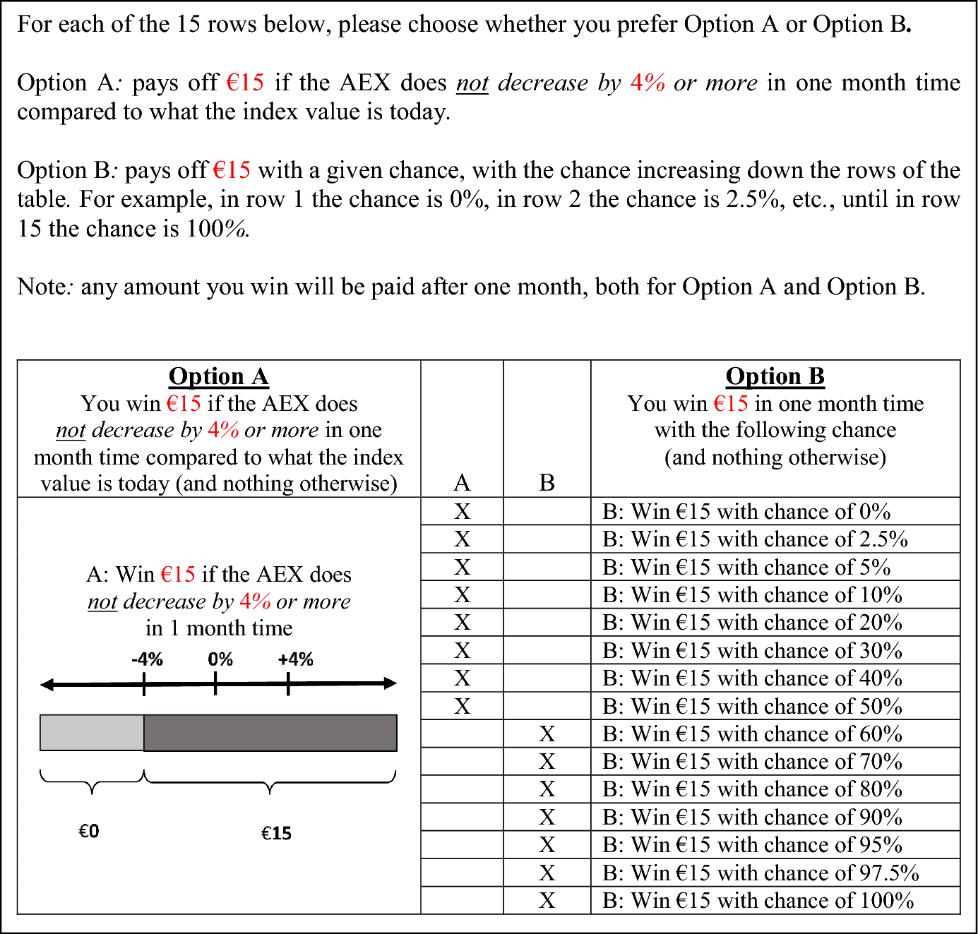
Fig. 2 Second Choice List for Eliciting Ambiguity Attitudes about the AEX Index
A key insight of the method is that, for an ambiguity neutral decision maker, the matching probabilities of an event and its complement add up to 1 (
 , but under ambiguity aversion, the sum is less than 1 (
 ). For example, the choices in Figs. 1 and 2 imply that
 , indicating ambiguity aversion. Baillon et al. (Reference Baillon, Huang, Selim and Wakker2018b) define their ambiguity aversion index b, averaging over the three events, as follows:
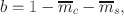
with
 Here
Here
 denotes the average single-event matching probability, and
 is the average composite-event matching probability. The decision-maker is ambiguity averse for
 , ambiguity seeking for
 , and ambiguity neutrality implies
 .
.
In practice, ambiguity attitudes have a second component apart from ambiguity aversion, namely a tendency to treat all uncertain events as though they had a 50–50% chance, which is called ambiguity-generated insensitivity or a-insensitivity (Abdellaoui et al., Reference Abdellaoui, Baillon, Placido and Wakker2011; Tversky & Fox, Reference Tversky and Fox1995). For unlikely events, a-insensitivity leads to overweighting and more ambiguity-seeking choices. Empirical studies have shown that a-insensitivity is a typical feature of decision-making under ambiguity (Trautmann and van de Kuilen Reference Trautmann, van de Kuilen, Keren and Wu2015; Dimmock et al., Reference Dimmock, Kouwenberg and Wakker2016a). Baillon et al. (Reference Baillon, Huang, Selim and Wakker2018b) define the following index to measure a-insensitivity:
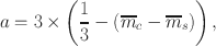
with
 For ambiguity neutral decision-makers,
 , while
 denotes a-insensitivity. Negative values,
 , indicate that the decision-maker is overly sensitive to changes in likelihood, implying underweighting of unlikely events.
In the neo-additive ambiguity model of Chateauneuf et al. (Reference Chateauneuf, Eichberger and Grant2007), index a is also a measure of the decision maker’s perceived level of ambiguity about a source, as long as
 1 (see Dimmock et al., Reference Dimmock, Kouwenberg, Mitchell and Peijnenburg2015; Baillon et al., Reference Baillon, Bleichrodt, Keskin, I’Haridon and Li2018a; and Online Appendix A). When
 the respondent has violated monotonicity, as then the average matching probability of the single events exceeds the average for the composite events
 . We will later analyze how frequently such violations occur and how often index a falls within the boundaries
 1 where it can be interpreted as the level of perceived ambiguity.
The method of Baillon et al. (Reference Baillon, Huang, Selim and Wakker2018b) has two major advantages: first, risk preferences (both the utility and probability weighting function) cancel out in the comparison between Options A and B, so they do not need to be estimated to identify ambiguity attitudes (Dimmock et al., Reference Dimmock, Kouwenberg and Wakker2016a). Second, using events and their complements in the calculation of index b and a ensures that the unknown subjective probabilities drop out of the equation (Baillon et al., Reference Baillon, Bleichrodt, Li and Wakker2021). Accordingly, we can measure ambiguity aversion without knowing respondents’ subjective beliefs. This solves the important issue that, when observing a dislike of ambiguity, it is difficult to disentangle whether this is due to ambiguity aversion or pessimistic beliefs.
2.2.1 Implementation of the elicitation method in the CentERpanel
Our survey module for eliciting ambiguity attitudes started with one practice question in the same choice list format as Fig. 1, where the uncertain event for Option A was whether the temperature in Amsterdam at 3 p.m. one month from now would be more than 20 degrees Celsius. After the practice question, a set of questions followed for each investment asset: the AEX index, a familiar individual company stock, a foreign stock index (MSCI World), and a crypto-currency (Bitcoin). Six matching probabilities were measured for each investment separately, so that index b and a can be estimated. The order of the four sets of questions was randomized, as was the order of the six events. Our final ambiguity aversion measures are labelled b_aex, b_stock, b_msci, and b_bitcoin and our measures for a-insensitivity are labelled a_aex, a_stock, a_msci, and a_bitcoin. Furthermore, we define b_avg (a_avg) as the average of the four b-indexes (a-indexes).
Before beginning the questions about the individual stock, each respondent was first asked to name a familiar company stock; subsequently, that stock name was used in the six choice lists shown to the respondent. For those who indicated they did not know any familiar company stock, we used Philips, a well-known Dutch consumer electronics brand. For the well-diversified AEX Index and the MSCI World Index, the event
 (
(
 ) represented a return of 4% (-4%) in one month. For the individual stock, the percentage change was set to 8% and forBitcoin to 30%, to reflect the higher historical volatility of these investments.Footnote 11
2.3 Elicitation of risk attitudes
The module also included four separate choice lists to measure risk attitudes (a screenshot is provided in Online Appendix B). The first risk attitude choice list elicited a certainty equivalent for a known 50% chance of winning €15 or €0 otherwise, based on a fair coin toss. The other three choice lists elicited a certainty equivalent for winning chances of €15 of 33%, 17%, and 83%, respectively, using a die throw. Respondents could win real money for the risk questions, and the order was randomized of the risk and ambiguity question sets in the survey.
Following Abdellaoui et al. (Reference Abdellaoui, Baillon, Placido and Wakker2011), we use index b r for risk as a measure of Risk Aversion, and index a r for risk as a measure of Likelihood Insensitivity, which is the tendency to treat all known probabilities as 50–50% and thus overweight small-probability events. To estimate these measures, we assume a rank-dependent utility model with a neo-additive probability weighting function and a linear utility function. We do this for two reasons. First, these two risk attitude measures are conceptually related to index b for ambiguity aversion and index a for a-insensitivity (Abdellaoui et al., Reference Abdellaoui, Baillon, Placido and Wakker2011). Second, utility curvature is often close to linear for small payoffs. We refer to Online Appendix C for more details about these measures, and for a robustness check using two non-parametric risk measures that do not rely on any model assumptions.
The Appendix Table 1 shows that on average investors were risk averse (mean > 0) but with strong heterogeneity, and about one third of the investors were risk seeking. Further, the Likelihood Insensitivity measure is positive for 85% of the investors, indicating a tendency to overweight small probabilities, in line with the findings of previous studies (see, e.g., Fehr-Duda & Epper, Reference Fehr-Duda and Epper2011 and Dimmock et al., Reference Dimmock, Kouwenberg, Mitchell and Peijnenburg2021).
2.4 Real incentives
At the outset of the survey, each subject was told that one of his or her choices in the ambiguity and risk questions would be randomly selected and played for real money. Hence all respondents who completed the survey had a chance to win a prize based on their choices, and a total of €2,758 in real incentives was paid out. The incentives were determined and paid by CentERdata one month after the end of the survey, when the changes in the asset values were known. As panel members regularly receive payments for their participation, the involvement of CentERdata minimizes subjects’ potential concerns about the credibility of the incentives.
2.5 Financial literacy and asset ownership
Our survey module also collected data on financial literacy and asset ownership. Financial literacy is one of our key independent variables, as we aim to assess whether financial knowledge relates to ambiguity attitudes. To measure this, we use 12 questions from Lusardi and Mitchell (Reference Lusardi and Mitchell2007) and van Rooij et al. (Reference van Rooij, Lusardi and Alessie2011), shown in Online Appendix C. Financial Literacy is the number of correct responses to the 12 questions (the average is 10.6; see Appendix Table 1).Footnote 12
We validate our ambiguity measures by examining whether they relate to the financial assets owned by the investors. Our survey module asked the panel members whether they currently invested in the familiar company stock they mentioned, in mutual funds tracking the MSCI World index, or any crypto-currencies such as Bitcoin. Invests in Familiar Stock is an indicator variable equal to one if the investor currently held the familiar company stock, which 30.2% did (see Appendix Table 1). Invests in Crypto-Currencies and Invests in MSCI World are equal to one if the investor held any crypto-currencies or funds tracking the MSCI World stock index, which was true for 2.4% and 1.4%, respectively. Finally, none of the investors in the sample owned funds tracking the domestic AEX stock index.
We note that even in the group of financial assets owners we label as “investors,” ownership of the four assets presented in our ambiguity survey is rather low, as most only own some mutual funds or bonds. Further, only half (55%) in the investor group could name a listed company stock with which they were familiar. All of this indicates that financial sophistication is not that high on average among Dutch retail investors, as is typically found in other household finance studies as well (see Gomes et al., Reference Gomes, Haliassos and Ramadorai2021, for a review).
3 Results for ambiguity aversion
3.1 Descriptive statistics
Figure 3 shows the fraction of respondents who were ambiguity averse, neutral, and seeking, for the four sources of ambiguity: the familiar stock, the domestic stock market index (AEX), a foreign stock market index (MSCI World), and Bitcoin. To account for possible measurement error, we classify small values of index b that are not significantly different from zero as ambiguity neutral.Footnote 13 About 58% of the respondents were ambiguity averse, while 30% were ambiguity seeking, a pattern that is similar across the sources of financial ambiguity. Furthermore, ambiguity neutrality was less common (12%), implying that only few investors’ choices were consistent with the expected utility model. Our results confirm for real-world sources of uncertainty that ambiguity aversion is common, but not universal. These findings are comparable to earlier large-scale studies that used artificial sources, such as Dimmock et al. (Reference Dimmock, Kouwenberg, Mitchell and Peijnenburg2015), Dimmock et al., (Reference Dimmock, Kouwenberg and Wakker2016a), and Kocher et al. (Reference Kocher, Lahno and Trautmann2018), showing that ambiguity seeking choices are not limited to Ellsberg urns.
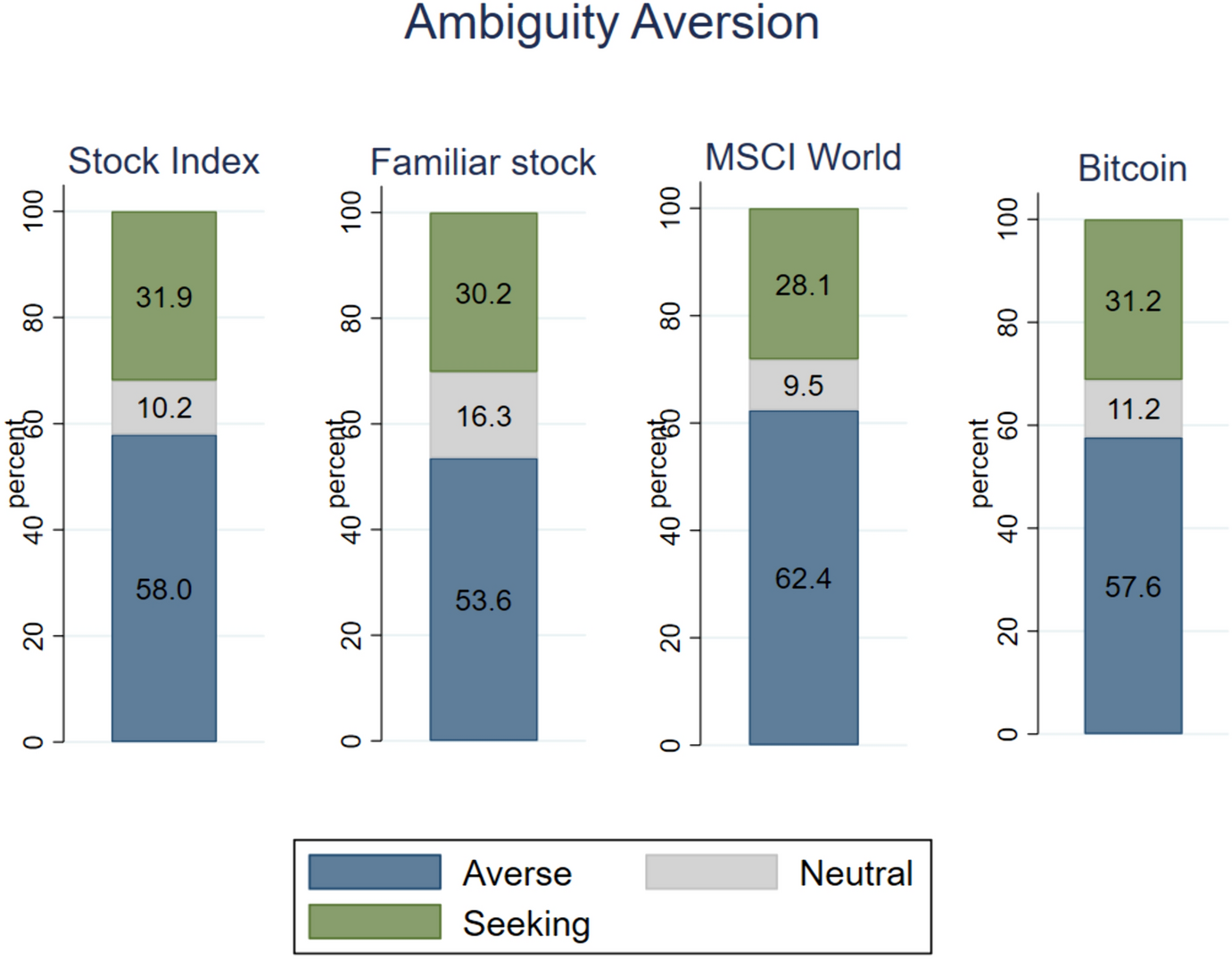
Fig. 3 Ambiguity Attitudes toward Financial Sources (Averse, Neutral and Seeking). This Figure shows the percent of investors who are ambiguity averse (b-index > 0, significant at 5%), ambiguity neutral (cannot reject b-index = 0), and ambiguity seeking (b-index < 0, significant at 5%) for the local stock market index (b_aex), a familiar company stock (b_stock), the MSCI World stock index (b_msci), and Bitcoin (b_bitcoin). The sample consists of n = 295 investors
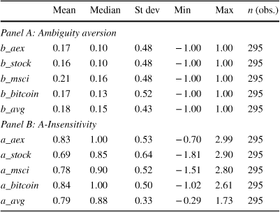
Table 1 shows descriptive statistics for the b-indexes. Investors on average display higher ambiguity aversion toward the foreign stock index (0.21), compared to the domestic AEX index (0.17), the familiar individual stock (0.16), and Bitcoin (0.17), in line with the well-document home bias (French & Poterba, Reference French and Poterba1991). There was strong heterogeneity in ambiguity aversion between investors, as indicated by the high standard deviation of the b-indexes (about 0.5 on average). We use Hotelling’s T-squared statisticFootnote 14 to test the hypothesis that the mean b-index is equal for the four investments, which cannot be rejected at the 5% level (T 2 = 7.65; p = 0.057). This implies that the mean level of ambiguity aversion does not depend strongly on the source of financial uncertainty. This is in line with Baillon and Bleichrodt (Reference Baillon and Bleichrodt2015), who found that Dutch financial-economics students did not display source preference for the AEX over the Indian SENSEX index. Still, in our sample, ambiguity aversion for the familiar stock (0.16) is 34% lower compared to the MSCI World index (0.21; p = 0.009 for the mean difference), so investors on aggregate did display some source preference for the familiar stock over a foreign stock market index.
Table 1 Descriptive Statistics for Ambiguity Attitudes
|
Mean |
Median |
St dev |
Min |
Max |
n (obs.) |
|
|---|---|---|---|---|---|---|
|
Panel A: Ambiguity aversion |
||||||
|
b_aex |
0.17 |
0.10 |
0.48 |
− 1.00 |
1.00 |
295 |
|
b_stock |
0.16 |
0.10 |
0.48 |
− 1.00 |
1.00 |
295 |
|
b_msci |
0.21 |
0.16 |
0.48 |
− 1.00 |
1.00 |
295 |
|
b_bitcoin |
0.17 |
0.13 |
0.52 |
− 1.00 |
1.00 |
295 |
|
b_avg |
0.18 |
0.15 |
0.43 |
− 1.00 |
1.00 |
295 |
|
Panel B: A-Insensitivity |
||||||
|
a_aex |
0.83 |
1.00 |
0.53 |
− 0.70 |
2.99 |
295 |
|
a_stock |
0.69 |
0.85 |
0.64 |
− 1.81 |
2.90 |
295 |
|
a_msci |
0.78 |
0.90 |
0.52 |
− 1.51 |
2.80 |
295 |
|
a_bitcoin |
0.84 |
1.00 |
0.50 |
− 1.02 |
2.61 |
295 |
|
a_avg |
0.79 |
0.88 |
0.33 |
− 0.29 |
1.73 |
295 |
Panel A shows summary statistics for ambiguity aversion regarding the local stock market index (b_aex), a familiar company stock (b_stock), the MSCI World stock index (b_msci) and Bitcoin (b_bitcoin), as well as the average of the four b-indexes (b_avg). Positive values of the b-index denote ambiguity aversion, and negative values indicate ambiguity seeking. Panel B shows summary statistics of index a (a-insensitivity) for the local stock market index (a_aex), a familiar company stock (a_stock), the MSCI World stock index (a_msci) and Bitcoin (a_bitcoin), as well as the average of the four a-indexes (a_avg). The sample consists of n = 295 investors
Figure 4 illustrates the relation between the ambiguity aversion measures for the four different investment sources at the subject level, shown with scatter plots. The correlations are all relatively strong, ranging between 0.62 and 0.74. This implies that if an investor had relatively high ambiguity aversion toward one specific financial source (e.g., the AEX index), he also tended to display high ambiguity aversion toward the other three investments. A factor analysis shows that the first factor explains 77% of the cross-sectional variation in the four ambiguity aversion measures, indicating that a single underlying variable is driving most of the variation.
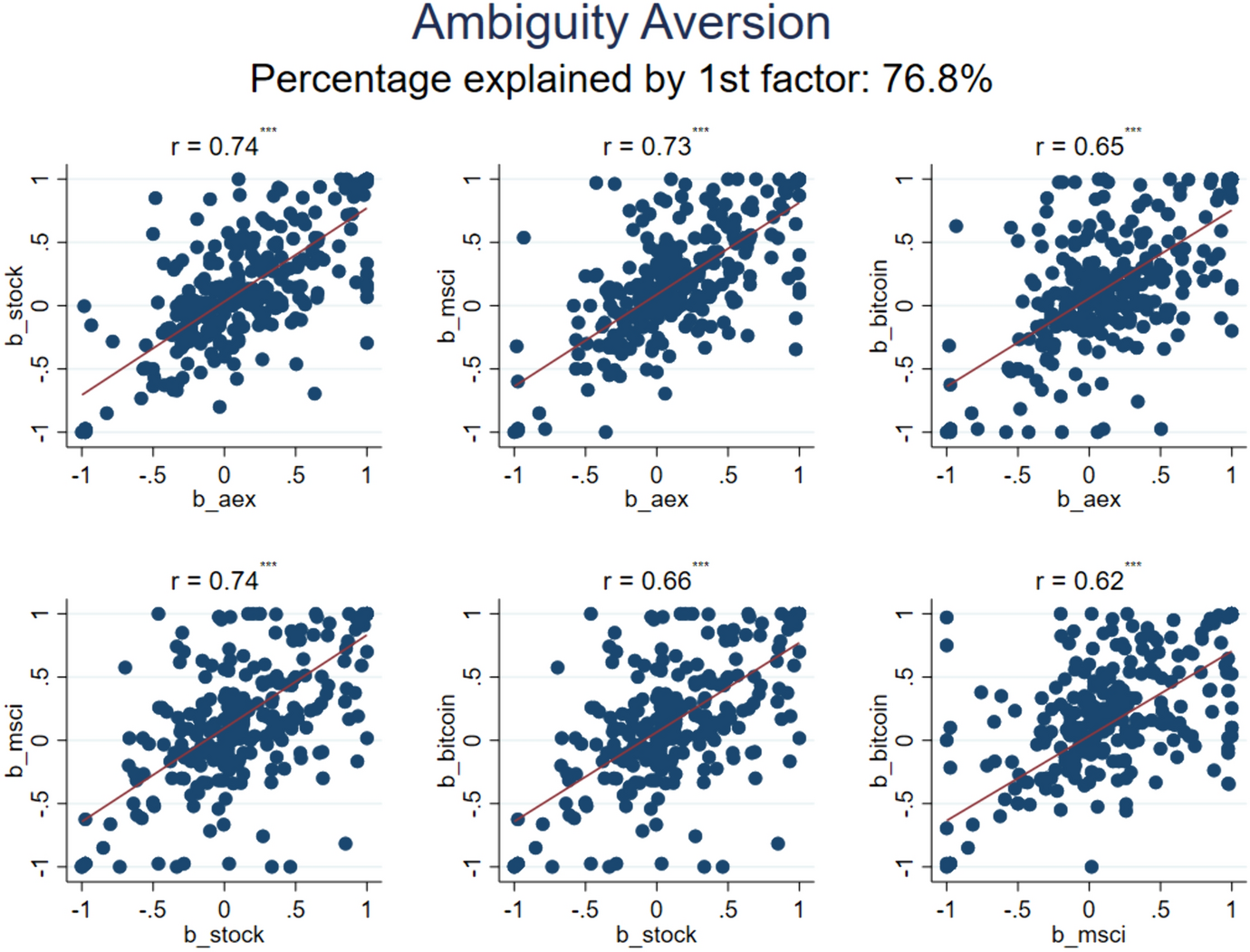
Fig. 4 Scatter Plots of Ambiguity Attitudes toward Different Financial Sources. This Figure shows scatter plots of the relationships between ambiguity aversion (the b-indexes) for different investments: the local stock market index (b_aex), a familiar company stock (b_stock), the MSCI World stock index (b_msci), and Bitcoin (b_bitcoin). The correlation (r) is shown above each scatter plot, with *, **, *** denoting significance at the 10%, 5% and 1%, respectively. The sample consists of n = 295 investors
3.2 Econometric model
Previous empirical studies by Borghans et al. (Reference Borghans, Heckman, Golsteyn and Meijers2009), Stahl (Reference Stahl2014), and l’Haridon et al. (Reference I’Haridon, Vieider, Aycinena, Bandur, Belianin, Cingl, Kothiyal and Martinsson2018) found high levels of unexplained heterogeneity in ambiguity attitudes when measured with Ellsberg urns, which l’Haridon et al. (Reference I’Haridon, Vieider, Aycinena, Bandur, Belianin, Cingl, Kothiyal and Martinsson2018) interpreted as noise (e.g., errors or random responses). An open question is: to what extent does using real-world investments help to improve measurement reliability? In this section, we analyze the variation in ambiguity attitudes using econometric models, following the approach of Dimmock et al. (Reference Dimmock, Kouwenberg, Mitchell and Peijnenburg2015) and l’Haridon et al. (Reference I’Haridon, Vieider, Aycinena, Bandur, Belianin, Cingl, Kothiyal and Martinsson2018). We estimate a panel regression model, where the cross-sectional unit i is the individual respondent, and the “time dimension” s (or repeated measurement) comes from the four investments:

where
 is index b (ambiguity aversion) of respondent i toward source s, for the AEX index (s = 1), the familiar stock (s = 2), the MSCI World index (s = 3), and Bitcoin (s = 4).
The dummy variable
 is 1 for source s, and 0 otherwise. The constant
 represents ambiguity aversion for the AEX index, whereas the coefficients
 and
and
 for the familiar stock, MSCI World and Bitcoin represent differences in mean ambiguity aversion relative to the AEX index. A set of K observable individual characteristics
 , such as age and gender, can also impact ambiguity aversion, with regression slope coefficients
 . The error term
 is identically and independently distributed, with
 .
.
Random effect
 represents unobserved heterogeneity in ambiguity aversion, which is independent of the error term and uncorrelated between individuals, with
 . Further, random effect
 is known as a “random slope” (with
 ), as it changes the beta of the source dummy
 . For example,
 captures individual heterogeneity in ambiguity aversion toward the familiar stock (s = 2), in addition to the heterogeneity in ambiguity aversion that affects all sources captured by the “random constant”
 . Correlations between random effects (
 ,
,
 ) are also estimated as part of the model.
The total variance of ambiguity attitudes can now be decomposed as follows:Footnote 15

with the four right-hand-side components representing variance explained by observed variables, unobserved individual heterogeneity in ambiguity attitudes that is common to all sources (
 ), unobserved source-specific individual heterogeneity (
 , and random errors (
 .
.
Our estimation approach is as follows: first, we estimate a model with only a random constant, and then random slopes are added to the model one at a time, followed by a test for their significance (a likelihood-ratio test).Footnote 16 Suppose
 (familiar stock) and
 (Bitcoin) are significant individually: then a model with both random slopes is estimated and tested as well. Finally, if an estimated random slope model turns out to have insignificant variance (
 ), or perfect correlation with the random constant (
 = 1 or -1), then it is considered invalid and not used.
3.3 Analysis of heterogeneity in ambiguity aversion
The estimation results for index b, ambiguity aversion, appear in Table 2. The sample consists of all 295 investors. All values of index
 are included, even if the respondent violated monotonicity or made other errors, to show the impact of noise in the data. Model 1 in Table 2 includes only a random effect capturing individual heterogeneity in ambiguity aversion that is common to the four investments, which explains 69% of the variation. The constant in the model is 0.177 (p < 0.001), implying that investors on average are ambiguity averse toward the investments. Table 2 also reports the interclass correlation coefficient (ICC), which in our dataset captures the correlation of ambiguity aversion toward the four sources.Footnote 17 The ICC is 0.69, indicating that the correlation in ambiguity aversion for the four investments is high.
Table 2 Analysis of Heterogeneity in Ambiguity Aversion

|
Dependent variable: ambiguity aversion (Index b) |
|||||
|---|---|---|---|---|---|
|
Model 1 |
Model 2 |
Model 3 |
Model 4 |
Model 5 |
|
|
Constant |
0.177*** |
0.168*** |
0.168*** |
0.153 |
0.212 |
|
(0.025) |
(0.028) |
(0.028) |
(0.219) |
(0.240) |
|
|
Dummy Familiar stock |
− 0.012 |
− 0.012 |
− 0.012 |
− 0.012 |
|
|
(0.020) |
(0.020) |
(0.020) |
(0.020) |
||
|
Dummy MSCI World |
0.042** |
0.042** |
0.042** |
0.042** |
|
|
(0.021) |
(0.021) |
(0.021) |
(0.021) |
||
|
Dummy Bitcoin |
0.007 |
0.007 |
0.007 |
0.007 |
|
|
(0.024) |
(0.024) |
(0.024) |
(0.024) |
||
|
Education |
− 0.010 |
− 0.018 |
|||
|
(0.017) |
(0.016) |
||||
|
Age |
0.006*** |
0.003* |
|||
|
(0.002) |
(0.002) |
||||
|
Female |
0.072 |
0.059 |
|||
|
(0.062) |
(0.053) |
||||
|
Single |
− 0.116** |
− 0.090* |
|||
|
(0.058) |
(0.049) |
||||
|
Employed |
− 0.040 |
− 0.042 |
|||
|
(0.070) |
(0.058) |
||||
|
Number of Children (log) |
0.059 |
0.048 |
|||
|
(0.062) |
(0.057) |
||||
|
Family income (log) |
− 0.011 |
0.016 |
|||
|
(0.014) |
(0.016) |
||||
|
HH Fin. Wealth (log) |
− 0.016* |
− 0.011* |
|||
|
(0.009) |
(0.007) |
||||
|
HH wealth imputed |
− 0.130 |
− 0.050 |
|||
|
(0.115) |
(0.092) |
||||
|
Financial literacy |
− 0.015 |
||||
|
(0.017) |
|||||
|
Risk aversion |
0.466*** |
||||
|
(0.065) |
|||||
|
Likelihood insensitivity |
− 0.084* |
||||
|
(0.048) |
|||||
|
Random slope: bitcoin |
No |
No |
Yes |
Yes |
Yes |
|
Observations n |
1180 |
1180 |
1180 |
1180 |
1180 |
|
ICC of Random effect
|
0.69 |
0.69 |
0.74 |
0.72 |
0.65 |
|
|
0.075 (31%) |
0.075 (31%) |
0.061 (25%) |
0.061 (25%) |
0.061 (25%) |
|
|
0.165 (69%) |
0.165 (69%) |
0.167 (70%) |
0.152 (63%) |
0.112 (47%) |
|
|
– |
– |
0.011 (5%) |
0.012 (5%) |
0.012 (5%) |
|
|
– |
0.0004 (0%) |
0.0004 (0%) |
0.015 (6%) |
0.056 (23%) |


The table shows estimation results for the panel regression model in Eq. (3), with index b (ambiguity aversion) toward the four investments as the dependent variable. Model 1 includes a constant and a random effect for individual-level heterogeneity in ambiguity aversion common to all sources. Model 2 adds dummies for differences in mean b between the four investments. Model 3 includes a random slope to capture heterogeneity in ambiguity aversion toward Bitcoin, shown to be significant by a likelihood ratio test (see Online App. E.1). Model 4 includes education, age, gender, single, employment, log number of children, family income, and household financial wealth, plus a missing wealth dummy. Model 5 adds financial literacy, risk aversion and likelihood insensitivity. Sample: n = 1180 observations of index b, for 295 investors. Standard errors clustered by investor shown in parentheses
Model 2 adds dummies to allow for differences in the mean level of ambiguity aversion toward the four investments. The dummy for the MSCI World index is positive (p = 0.042), implying investors are more ambiguity averse toward foreign stocks. Random slopes for source-specific ambiguity aversion are added next, and a chi-square test (reported in Online Appendix E.1) shows that only adding a random slope for Bitcoin leads to an improvement of model fit (p < 0.001). Heterogeneity in ambiguity aversion toward Bitcoin (the random slope) explains 5% of the variation in Model 3, on top of the 70% captured by ambiguity aversion toward all four sources (random constant). Overall, the results imply that ambiguity aversion toward investments is driven mainly by one underlying factor, with high correlation between measurements for different sources.
3.4 Variation in ambiguity attitudes explained by individual characteristics
Model 4 in Table 2 adds observed individual socio-demographic variables such as age, gender, education, employment, income, and financial assets, which together account for about 6% of the variation. Ambiguity aversion toward investments is lower for younger investors (p = 0.008) and singles (p = 0.044). In Model 5, proxies for financial literacy and risk attitudes are added, which account for an additional 17% of the variation. Specifically, ambiguity aversion toward investments and risk aversion are positively related (p < 0.001). Ambiguity aversion is not related to financial literacy and also not lower for the familiar stock, suggesting limited competence effects (Heath & Tversky, Reference Heath and Tversky1991) in ambiguity aversion for investments.
All observed variables together explain 23% of the variation in ambiguity aversion in Model 4, while 52% is driven by unobserved heterogeneity (of which 5% specific to the Bitcoin source), and the remaining 25% is error. The relatively low percentage attributed to error suggests that measurement reliability is relatively high for ambiguity aversion toward investments.
4 Results for a-insensitivity and perceived ambiguity
4.1 Descriptive statistics
Panel B of Table 1 summarizes the a-index values. On average, a-insensitivity is high (0.79), implying that investors do not much discriminate between single and composite events, suggesting they perceive high ambiguity about their probabilities.Footnote 18 Further tests show that the mean of index a is significantly lower for the familiar stock (0.69).
Overall, the large majority of investors is insensitive to the likelihood of ambiguous events (a > 0) for the four investment sources, as shown in Panel A of Table 3. Hence, a-insensitivity is common, in line with earlier results for stocks in Fox et al. (Reference Fox, Rogers and Tversky1996) and Kilka and Weber (Reference Kilka and Weber2001), but we can now confirm this in a large field study of investors, using measurements that control for beliefs and risk preferences. These findings are also in line with results for Ellsberg urns in Dimmock et al. (Reference Dimmock, Kouwenberg, Mitchell and Peijnenburg2015) and Dimmock et al., (Reference Dimmock, Kouwenberg and Wakker2016a).
Table 3 Descriptive Statistics for Perceived Ambiguity
|
Within limits for perceived ambiguity |
Over-sensitive to likelihoods |
Violation of monotonicity |
|
|---|---|---|---|
|
% with 0 ≤ a ≤ 1 |
% with a < 0 |
% with a > 1 |
|
|
Panel A: Negative values of index a and violations of monotonicity |
|||
|
a_aex |
65.1 |
8.8 |
26.1 |
|
a_stock |
65.1 |
12.5 |
22.4 |
|
a_msci |
69.5 |
7.8 |
22.7 |
|
a_bitcoin |
69.5 |
5.4 |
25.1 |
|
a_avg |
77.6 |
2.0 |
20.3 |
|
Mean |
Median |
St. dev. |
Min |
Max |
n (obs.) |
|
|---|---|---|---|---|---|---|
|
Panel B: Summary statistics of perceived ambiguity |
||||||
|
a_aex |
0.74 |
0.89 |
0.30 |
0.00 |
1.00 |
192 |
|
a_stock |
0.64 |
0.74 |
0.35 |
0.01 |
1.00 |
192 |
|
a_msci |
0.72 |
0.80 |
0.30 |
0.00 |
1.00 |
205 |
|
a_bitcoin |
0.75 |
0.91 |
0.30 |
0.01 |
1.00 |
205 |
|
a_avg |
0.71 |
0.76 |
0.26 |
0.02 |
1.00 |
229 |
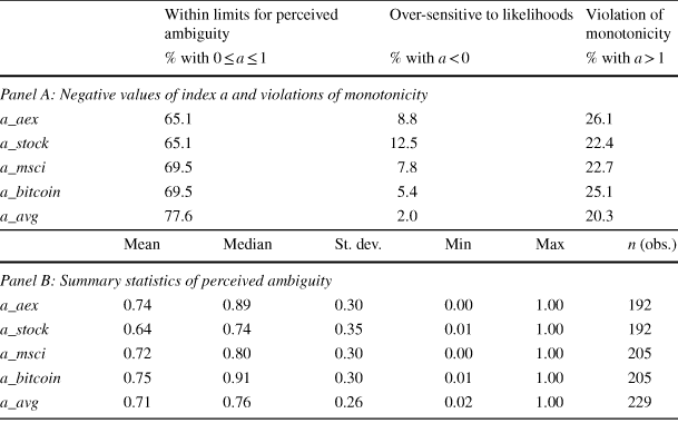
The table shows summary statistics for index a, for the local stock market index (a_aex), a familiar company stock (a_stock), the MSCI World stock index (a_msci) and Bitcoin (a_bitcoin), as well as the average of the four a-indexes (a_avg). Panel A of the table shows the percentage of a-index values that are negative (over-sensitive to likelihoods), between 0 and 1 (in line with the interpretation of index a as perceived ambiguity), and larger than 1 (violations of monotonicity). The sample consists of n = 295 investors. In Panel B, the sample has been restricted to only those observations of index a that are between 0 and 1, after pairwise deletion, so that the a-indexes can be interpreted as measures of perceived ambiguity. For this reason, in Panel B the sample size varies, as indicated in the last column
Panel A of Table 3 shows about two thirds of the a-index values fell in the range 0 to 1, such that they can be interpreted as the perceived level of ambiguity. About 25% of the respondents had a > 1 and thus violated monotonicity when looking at each investment separately, and 20% after averaging over the four investments (a_avg > 1). Earlier studies such as Li et al. (Reference Li, Müller, Wakker and Wang2018) and Dimmock et al., (Reference Dimmock, Kouwenberg and Wakker2016a) found similar rates of monotonicity violations, as summarized in Sect. 5.4.2.
As we aim to interpret index a as a proxy for perceived ambiguity, from now on we exclude monotonicity violations (a > 1) and negative values of a, using pairwise deletion.Footnote 19 Panel B of Table 3 shows descriptive statistics for perceived ambiguity. On average, investors perceived less ambiguity about the familiar individual stock (0.64) than toward the foreign index (0.72), the domestic stock index (0.74), and Bitcoin (0.75).Footnote 20 We note that perceived ambiguity about investments is relatively high, at 0.71 on average. For comparison, in Dimmock et al., (Reference Dimmock, Kouwenberg and Wakker2016a), perceived ambiguity toward Ellsberg urns was 0.35 on average.
There are several reasons why perceived ambiguity about investment can be expected to be high in our field study. First, the household finance literature shows that typical retail investors are not sophisticated, lack financial knowledge, and suffer from a host of biases (see Gomes et al., Reference Gomes, Haliassos and Ramadorai2021 for a review). In line with this, even in the group of financial asset owners that we labelled as investors, only 55% could mention a familiar stock name, and less than half owned individual stocks. Second, the probabilities of the one-month investment return events are hard to estimate, as both the mean and standard deviation are time-varying (Lettau & Ludvigson, Reference Lettau, Ludvigson, Ait-Sahalia and Hansen2010), requiring quite a high level of financial sophistication. Finally, our choice lists do not reveal any information about the event probabilities; a respondent who always selects the middle row due to lack of knowledge or attention will end up with an a-index equal to one (100%).Footnote 21
Figure 5 shows scatter plots of the relations between perceived ambiguity toward the four financial sources. The correlations between the a-indexes are positive, ranging from 0.35 to 0.55, but lower than correlations between the b-indexes. A factor analysis indicates that the first component accounts for about 60% of the cross-sectional variation in the four measures. This implies that, for a given respondent, the perceived ambiguity toward different investments is related, but not strongly. Hence, the same investor may perceive relatively low ambiguity about a familiar stock, while concurrently perceiving high ambiguity about another investment.Footnote 22
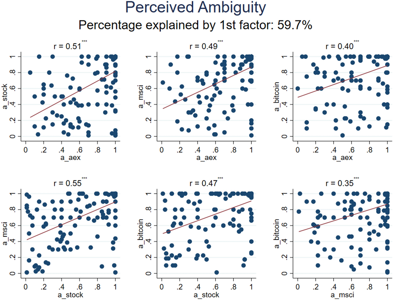
Fig. 5 Scatter Plots of Perceived Ambiguity about Different Financial Sources. This Figure shows scatter plots of the relation between perceived ambiguity (the a-indexes) for different investments: the local AEX stock market index (a_aex), a familiar company stock (a_stock), the MSCI World stock index (a_msci), and Bitcoin (a_bitcoin). The correlation (r) is shown above each scatter plot, with *, **, *** denoting significance at the 10%, 5% and 1%, respectively. The original sample consists of n = 295 investors, but values of index a that are negative or larger than 1 are excluded pairwise
4.2 Analysis of heterogeneity in perceived ambiguity
We now analyze the variance in perceived ambiguity, using a similar panel model as above:

where
 is index a (perceived ambiguity) of respondent i toward source s, with
 . The constant
 represents perceived ambiguity for the AEX index, whereas the coefficients
 and
and
 for the familiar stock, MSCI World and Bitcoin represent differences in the mean relative to the AEX. The random effect and the error term are denoted by
 and
and
 , respectively, whereas
 represents random slopes (added if significant based on a likelihood ratio test).
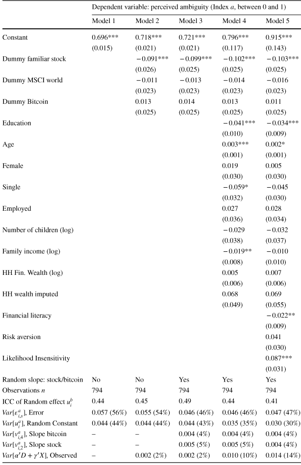
Table 4 shows the estimation results. Model 1 includes only a random effect, capturing individual heterogeneity in perceived ambiguity that is common to the four sources, which explains 44% of the variation. Model 2 shows that investors perceive less ambiguity about the familiar stock,
 = -0.091 (p < 0.001), relative to
 = 0.718 for the other investments on average. The ICC is 0.45, implying that levels of perceived ambiguity toward the four different investments have a moderate positive correlation.
Table 4 Analysis of Heterogeneity in Perceived Ambiguity
|
Dependent variable: perceived ambiguity (Index a, between 0 and 1) |
|||||
|---|---|---|---|---|---|
|
Model 1 |
Model 2 |
Model 3 |
Model 4 |
Model 5 |
|
|
Constant |
0.696*** |
0.718*** |
0.721*** |
0.796*** |
0.915*** |
|
(0.015) |
(0.021) |
(0.021) |
(0.117) |
(0.143) |
|
|
Dummy familiar stock |
− 0.091*** |
− 0.099*** |
− 0.102*** |
− 0.103*** |
|
|
(0.026) |
(0.025) |
(0.025) |
(0.025) |
||
|
Dummy MSCI world |
− 0.011 |
− 0.013 |
− 0.014 |
− 0.016 |
|
|
(0.023) |
(0.023) |
(0.023) |
(0.023) |
||
|
Dummy Bitcoin |
0.013 |
0.014 |
0.013 |
0.011 |
|
|
(0.025) |
(0.025) |
(0.025) |
(0.025) |
||
|
Education |
− 0.041*** |
− 0.034*** |
|||
|
(0.010) |
(0.009) |
||||
|
Age |
0.003*** |
0.002* |
|||
|
(0.001) |
(0.001) |
||||
|
Female |
0.019 |
0.005 |
|||
|
(0.030) |
(0.030) |
||||
|
Single |
− 0.059* |
− 0.045 |
|||
|
(0.032) |
(0.030) |
||||
|
Employed |
0.027 |
0.028 |
|||
|
(0.036) |
(0.034) |
||||
|
Number of children (log) |
− 0.029 |
− 0.032 |
|||
|
(0.038) |
(0.037) |
||||
|
Family income (log) |
− 0.019** |
− 0.010 |
|||
|
(0.008) |
(0.010) |
||||
|
HH Fin. Wealth (log) |
0.005 |
0.007 |
|||
|
(0.006) |
(0.006) |
||||
|
HH wealth imputed |
0.068 |
0.069 |
|||
|
(0.049) |
(0.055) |
||||
|
Financial literacy |
− 0.022** |
||||
|
(0.009) |
|||||
|
Risk aversion |
0.041 |
||||
|
(0.030) |
|||||
|
Likelihood Insensitivity |
0.087*** |
||||
|
(0.031) |
|||||
|
Random slope: stock/bitcoin |
No |
No |
Yes |
Yes |
Yes |
|
Observations n |
794 |
794 |
794 |
794 |
794 |
|
ICC of Random effect
|
0.44 |
0.45 |
0.49 |
0.44 |
0.41 |
|
|
0.057 (56%) |
0.055 (54%) |
0.046 (46%) |
0.046 (46%) |
0.047 (47%) |
|
|
0.044 (44%) |
0.044 (44%) |
0.044 (43%) |
0.035 (35%) |
0.030 (30%) |
|
|
– |
– |
0.004 (4%) |
0.004 (4%) |
0.004 (4%) |
|
|
– |
– |
0.005 (5%) |
0.005 (5%) |
0.004 (4%) |
|
|
– |
0.002 (2%) |
0.002 (2%) |
0.010 (10%) |
0.014 (14%) |


The table shows estimation results for the panel regression model in Eq. (5), with index a toward the four investments as dependent variable. Only values of index a between 0 and 1 are included, so index a can be interpreted as perceived ambiguity. Model 1 includes a constant and a random effect for individual-level heterogeneity in perceived ambiguity common to all sources. Model 2 adds dummies for differences in the mean of perceived ambiguity between investments. Model 3 includes a random slope to capture heterogeneity in perceived ambiguity toward the familiar stock and Bitcoin (see Online App. E.2). Model 4 includes observed socio-demographic variables. Model 5 adds financial literacy, risk aversion and likelihood insensitivity. Sample: n = 794 observations of perceived ambiguity (a-index values between 0 and 1), for 295 investors. Standard errors clustered by investor in parentheses.
Next, including random slopes for the familiar stock and Bitcoin in Model 3 leads to a significant improvement of model fit (see Online Appendix E.2). Individual variation in perceived ambiguity toward the familiar stock explains 5% of the total variation, versus 4% for Bitcoin, on top of the 43% captured by general perceived ambiguity about all investments (random constant). Hence, whereas ambiguity aversion is mostly driven by one underlying preference variable, perceived levels of ambiguity tend to differ more depending on the specific source considered.
4.3 Variation in perceived ambiguity explained by individual characteristics
Model 4 adds observed individual socio-demographic variables to the model, which account for 8% of the variation (= 10–2%) in perceived ambiguity. Older investors perceive more ambiguity about investments (p = 0.005), whereas investors with higher education (p < 0.001) and more income (p = 0.026) perceive less ambiguity. Model 5 adds proxies for financial literacy and risk attitudes, which explain an additional 4%. Specifically, investors with better financial literacy perceive less ambiguity (p = 0.011). Further, perceived ambiguity is positively related to index a r for risk (p = 0.005), a proxy for likelihood insensitivity. All variables together explain 14% of the variation, whereas 38% is driven by unobserved heterogeneity, and 47% is error. Together, the results indicate that measurement reliability for perceived ambiguity is reasonable, although clearly lower than for ambiguity aversion. The likely reason is that index a is measured using differences in matching probabilities for composite events and single events (see Eq. (2)), and therefore more sensitive to errors and violations of monotonicity.
In Online Appendix F we repeat the analyses above using all values of index a, without screening out monotonicity violations and negative values: in that case the ICC is just 0.16 and measurement error accounts for 75% of the variation. The high level of noise implies that unfiltered a-insensitivity is strongly influenced by errors such as violations of monotonicity (a > 1). Further, screening out such violations leads to substantially better reliability for index a.
5 Validity of the measures
5.1 Relation with risk preferences, education and financial literacy
We assess the validity of the ambiguity measures by testing whether they relate to other variables in expected ways. For example, a priori we expect that ambiguity aversion is positively related to risk aversion, as that is the most common finding in previous studies summarized by Trautmann and van de Kuilen (Reference Trautmann, van de Kuilen, Keren and Wu2015) and Baillon et al. (Reference Baillon, Schlesinger and van de Kuilen2018c). Similarly, we expect that likelihood insensitivity (overweighting of small probabilities) is positively related to a-insensitivity (overweighting of unlikely events), and thus to perceived ambiguity. The results in Tables 2 and 4 confirm these relations (p < 0.01).Footnote 23
A priori, we also expect that investors with better financial knowledge and higher education perceive less ambiguity about the distribution of investment returns. Table 4 confirms both of these relations (p < 0.05), suggesting that more knowledge reduces the level of perceived ambiguity.Footnote 24 As an additional test, we also included a dummy for investors who named a specific stock they are familiar with (see Online Appendix G). As expected, investors naming a familiar stock perceive lower ambiguity about it (− 0.182; p < 0.001), compared to those answering questions about Philips.
The competence hypothesis of Heath and Tversky (Reference Heath and Tversky1991) predicts that ambiguity aversion is stronger when the decision maker feels less competent or less knowledgeable about the source, suggesting a negative relation between financial literacy and ambiguity aversion. The coefficient in Table 2 is negative as expected, but the effect is too small to be statistically significant.Footnote 25 Further, investors who named a specific familiar stock also did not display significantly lower ambiguity aversion to it (see Online Appendix G). Still, investors were significantly more ambiguity averse toward the foreign MSCI stock index in Table 2 compared to the domestic AEX index, displaying home bias (French & Poterba, Reference French and Poterba1991). In addition, the difference in ambiguity aversion for the familiar stock (b = 0.156) and the MSCI index (b = 0.210) is 34% in relative terms, a sizeable difference (p = 0.009). All in all, we find that there are strong competence effects in perceived ambiguity (a-insensitivity), but less so in ambiguity aversion.
5.2 The relation to investments
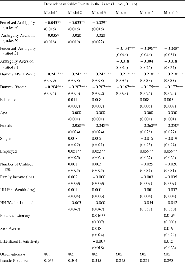
Next, we evaluate whether ambiguity attitudes correlate with actual investment choices. Based on theory, we expect that investments in risky assets are negatively affected by ambiguity aversion (Dow & Werlang Reference Dow and da Costa Werlang1992) and by the level of perceived ambiguity (Boyle et al., Reference Boyle, Garlappi, Uppal and Wang2012; Uppal & Wang, Reference Uppal and Wang2003). One caveat is that these relations also depend on how much ambiguity the investor perceives about all other available investment opportunities considered, for which we lack complete information. Further, many other unknown parameters also affect these relations, such as the investor’s subjective expectations about the return distribution of all available assets (mean, risk, skewness, and cross-correlations) and risk preferences. Although the exact signs are hard to predict, negative relations of index b and a with investments are what we expect to find on aggregate, based on earlier work by Dimmock et al., (Reference Dimmock, Kouwenberg and Wakker2016a).
We estimate a pooled probit model for asset ownership,
 , a dummy variable indicating ownership of the familiar stock (s = 2), the MSCI World index (s = 3), and Bitcoin (s = 4):

where indexes
 and
and
 have slope coefficients
 and
and
 . The constant
 represents average ownership of the familiar stock, whereas
 and
and
 indicate differences in ownership rates for MSCI World and Bitcoin. Investment in the AEX index (s = 1) is excluded, as noone in our sample invested in a fund tracking the AEX. The model includes K observable individual characteristics
 as control variables, with slope coefficients
 , for
, for
 .
.
The results in Model 1 of Table 5 show that index a has a negative relation with investing in an asset (p = 0.005). The coefficient of index b is also negative, as expected, but only marginally significant (p = 0.060). As more controls are added in Models 2 and 3, we note that the effect of index
 becomes smaller, probably because it is related to financial literacy and education.
Table 5 Investment in the Familiar Stock, MSCI World, and Crypto-Currencies
|
Dependent variable: Invests in the Asset (1 = yes, 0 = no) |
||||||
|---|---|---|---|---|---|---|
|
Model 1 |
Model 2 |
Model 3 |
Model 4 |
Model 5 |
Model 6 |
|
|
Perceived Ambiguity (index a) |
− 0.043*** |
− 0.033** |
− 0.029* |
|||
|
(0.015) |
(0.015) |
(0.015) |
||||
|
Ambiguity Aversion (index b) |
− 0.035* |
− 0.020 |
− 0.028 |
|||
|
(0.018) |
(0.019) |
(0.022) |
||||
|
Perceived Ambiguity (fitted
|
− 0.134*** |
− 0.096** |
− 0.088* |
|||
|
(0.046) |
(0.046) |
(0.051) |
||||
|
Ambiguity Aversion (fitted
|
− 0.018 |
− 0.004 |
− 0.018 |
|||
|
(0.024) |
(0.026) |
(0.032) |
||||
|
Dummy MSCI World |
− 0.241*** |
− 0.242*** |
− 0.242*** |
− 0.212*** |
− 0.218*** |
− 0.218*** |
|
(0.029) |
(0.028) |
(0.028) |
(0.035) |
(0.033) |
(0.033) |
|
|
Dummy Bitcoin |
− 0.204*** |
− 0.207*** |
− 0.207*** |
− 0.167*** |
− 0.175*** |
− 0.177*** |
|
(0.024) |
(0.023) |
(0.022) |
(0.028) |
(0.026) |
(0.026) |
|
|
Education |
0.011 |
0.008 |
0.008 |
0.005 |
||
|
(0.007) |
(0.007) |
(0.008) |
(0.008) |
|||
|
Age |
− 0.000 |
− 0.000 |
− 0.000 |
− 0.000 |
||
|
(0.001) |
(0.001) |
(0.001) |
(0.001) |
|||
|
Female |
− 0.058** |
− 0.048** |
− 0.062** |
− 0.050* |
||
|
(0.024) |
(0.024) |
(0.028) |
(0.027) |
|||
|
Single |
0.008 |
0.002 |
− 0.015 |
− 0.019 |
||
|
(0.022) |
(0.021) |
(0.025) |
(0.024) |
|||
|
Employed |
0.051** |
0.053** |
0.059** |
0.059** |
||
|
(0.025) |
(0.024) |
(0.027) |
(0.026) |
|||
|
Number of Children (log) |
0.001 |
0.003 |
− 0.025 |
− 0.020 |
||
|
(0.025) |
(0.025) |
(0.031) |
(0.031) |
|||
|
Family Income (log) |
0.002 |
− 0.000 |
− 0.003 |
− 0.005 |
||
|
(0.009) |
(0.009) |
(0.009) |
(0.009) |
|||
|
HH Fin. Wealth (log) |
0.001 |
0.000 |
− 0.001 |
− 0.002 |
||
|
(0.004) |
(0.003) |
(0.004) |
(0.004) |
|||
|
HH Wealth Imputed |
− 0.063 |
− 0.060 |
− 0.054 |
− 0.042 |
||
|
(0.047) |
(0.047) |
(0.052) |
(0.050) |
|||
|
Financial Literacy |
0.016** |
0.015* |
||||
|
(0.007) |
(0.008) |
|||||
|
Risk Aversion |
0.018 |
0.019 |
||||
|
(0.024) |
(0.029) |
|||||
|
Likelihood Insensitivity |
− 0.007 |
0.015 |
||||
|
(0.018) |
(0.022) |
|||||
|
Observations n |
885 |
885 |
885 |
602 |
602 |
602 |
|
Pseudo R-square |
0.267 |
0.304 |
0.315 |
0.245 |
0.281 |
0.293 |


This table reports estimation results for a panel probit model explaining asset ownership with index a and b, see Eq. (6). The dependent variable is 1 if the respondent invests in the asset (familiar individual stock, MSCI World, or Bitcoin), and 0 otherwise. Investment in the AEX index is excluded, as no respondents hold an AEX fund. The data for ownership of the three assets is treated as a panel dataset similar to Tables 2 and 4, see model Eq. (6) in the text for details. The coefficients displayed are estimated marginal effects, with index a and b evaluated at the mean. Standard errors clustered by investor shown in parentheses. In Model 4, 5, and 6 index a and b are replaced by fitted values from the panel regression models in Tables 2 and 4, using specification Model 3 with source dummies and random slopes. Further, only observations with
 are included in Model 4–6, so that fitted a can be interpreted as perceived ambiguity. The set of control variables is the same as in Tables 2 and 4
To reduce the impact of measurement error, Models 4 to 6 of Table 5 use as independent variables the predicted values
 and
and
 of ambiguity aversion and perceived ambiguity from the estimated panel models in Tables 2 and 4 (Model 3).Footnote 26 Using the predicted values, we effectively remove the error terms
 and
and
 from index b and a. The sample in Models 4 to 6 is smaller, as it includes only observations with
 , similar to Table 4. The results in Model 4 confirm that investors who perceive more ambiguity about an asset are less likely to invest in it, while ambiguity aversion is not significant.
Online Appendix E.3 shows results for several model specification tests. First, adding a random effect to the panel probit model (6) does not add value, because ownership of different investments is not very correlated. Second, allowing ambiguity aversion and perceived ambiguity to have a different effect on each investment does not improve the model fit either. Online Appendix H.5 also reports estimates using a probit model for each investment separately, as a robustness check. The results show that higher perceived ambiguity is negatively related to investing in MSCI World and Bitcoin, but it is not significant for the familiar stock. Further, investors with higher ambiguity aversion (index b) are less likely to invest in Bitcoin. Overall, these results show that the ambiguity attitude measures have significant correlations with actual investment choices.
5.3 Robustness tests
We performed several additional robustness checks for our main results, reported in Online Appendix H. First, we repeated the main analysis after screening out investors who make mistakes on the ambiguity choice lists, by preferring Option A or B on every row. The main effect is that the mean level of index b drops, as the most common error is selecting the unambiguous Option B on every row of the choice list; this results in high values of index b.Footnote 27 Apart from that, the measurement reliability (ICC), the percentage of variance explained by observable variables, and the correlates of ambiguity attitudes are similar to the full-sample results.
Second, we repeated the main analysis after excluding values of b and a from subjects with many violations of set-inclusion monotonicity. Third, we excluded 30 respondents who spent less than 10 minutes on the ambiguity survey module, to screen out subjects who devoted insufficient attention to the questions. The results in Online Appendix H are similar to the main findings in Tables 2 and 4. Overall, the three robustness checks show that the main results are not driven by respondents who made many mistakes, or who spent little time on the ambiguity questions.
5.4 Cross-sample comparisons
5.4.1 Comparison with the sample of non-investors
Table 7 in Appendix Table 2 shows summary statistics for index b and a in the group of 230 non-investors who owned no financial assets. In the columns “Mean” and “Median,”stars indicate whether the estimate for non-investors is significantly different from the value for investors in Table 1. Non-investors display significantly higher a-insensitivity to the investment sources on average (a_avg) compared to investors, as expected. By contrast, their average ambiguity aversion (b_avg) is not different from investors. This is in line with our earlier conclusion that competence effects are most pronounced in a-insensitivity, the cognitive component of ambiguity attitudes.
Online Appendix D provides more detailed analyses of the non-investor group, using the econometric model. In the non-investor group, heterogeneity in ambiguity aversion is driven by a single underlying factor, while random slopes for Bitcoin and other sources are not significant. Further, perceived ambiguity toward different investment is also largely driven by one underlying factor, explaining 48% of the variation. The means of ambiguity aversion and perceived ambiguity are also not different between sources. Hence, non-investors make less distinction in ambiguity between investments, most likely due to high unfamiliarity with all types of investments.
5.4.2 Comparisons with related ambiguity studies using Ellsberg urns
In this section we compare our results to Dimmock et al. (Reference Dimmock, Kouwenberg and Wakker2016a, henceforth DKW), who measured index b and a with Ellsberg urns in a large sample of the Dutch population (the LISS panel). We restricted their original sample of 666 subjects to 126 investors owning some financial assets, using the same criteria for defining investors as in our own sample. Hence, both samples are representative for Dutch investors, but they differ in the sources of ambiguity: our study used investments, while DKW used Ellsberg urns.
First, we compare monotonicity violations. About 25% in our sample of investors violated monotonicity when looking at each investment separately, while in the DKW study with Ellsberg urns, 25.4% violated monotonicity. Similar rates are reported by Li et al. (Reference Li, Müller, Wakker and Wang2018), ranging from 14 to 28%, in a study using both artificial and natural sources. Thus, the rates of monotonicity violations we found are similar to those in previous ambiguity studies.Footnote 28
Regarding ambiguity aversion, the average of index b for Ellsberg urns in DKW is 0.14, similar to the average value of 0.18 that we find for investments. This suggests that the mean level of ambiguity aversion is not that source-dependent, also between artificial and real-world sources. However, perceived ambiguity toward the Ellsberg urn on average was 0.35 in DKW, considerably lower than the range of 0.64 to 0.75 for investments in Table 3. This reinforces our conclusion that perceived ambiguity is source-dependent, also between artificial and real-world sources.
The percentage of variation in ambiguity aversion explained by respondent characteristics in DKW was 2%, but the methodology used was different. A more direct comparison can be made to l’Haridon et al. (Reference I’Haridon, Vieider, Aycinena, Bandur, Belianin, Cingl, Kothiyal and Martinsson2018) and Dimmock et al. (Reference Dimmock, Kouwenberg, Mitchell and Peijnenburg2015), who also measured ambiguity attitudes with Ellsberg urns in large samples and applied panel regression models. In those studies, observed individual characteristics like gender and age explained at most 3% of the variation and correlations between repeated measurements of ambiguity aversion were rather low (ICC: 0.15–0.30). l’Haridon et al. (Reference I’Haridon, Vieider, Aycinena, Bandur, Belianin, Cingl, Kothiyal and Martinsson2018) argue that when most variation in ambiguity attitudes remains unexplained, it is likely driven by noise (mistakes, random responses, etc.). By contrast, in the present study using real-world sources, the ICC is 0.69 and up to 23% of the variation in ambiguity aversion is explained. This suggests that ambiguity aversion for natural sources measured with the Baillon et al. (Reference Baillon, Huang, Selim and Wakker2018b) method has higher reliability compared to traditional measures based on Ellsberg urns.Footnote 29
6 Conclusions
This paper measures ambiguity attitudes for relevant real-world sources of ambiguity in a large representative sample of investors, while controlling for unknown probability beliefs and risk preferences. One concern raised in the literature is that ambiguity measurements for artificial events such as Ellsberg urns are often noisy, and not related to individual characteristics and economic outcomes (see, e.g., Sutter et al., Reference Sutter, Kocher, Glätzle-Rützler and Trautmann2013; Stahl, Reference Stahl2014; and l’Haridon et al., Reference I’Haridon, Vieider, Aycinena, Bandur, Belianin, Cingl, Kothiyal and Martinsson2018). Focusing on investments, our results show that the reliability of ambiguity aversion for natural sources is high, measured using the new method of Baillon et al. (Reference Baillon, Huang, Selim and Wakker2018b), as correlations between repeated measures of ambiguity aversion are in the 0.6 to 0.8 range. Individual characteristics also are significantly correlated with ambiguity attitudes: thus, demographics, income, wealth, financial literacy, and risk aversion explain 23% of the variation in ambiguity aversion and 14% of perceived ambiguity. Perceived ambiguity is lower among investors with better financial literacy and higher education, while ambiguity aversion is positively related to risk aversion. We also confirm that investors who perceive higher ambiguity about a particular asset are less likely to invest in it, and investors with higher ambiguity aversion are less likely to invest in Bitcoin, showing that the new measures of ambiguity attitudes are correlated with actual investment choices.
Our results further indicate that ambiguity aversion toward different investments is largely driven by one underlying subject-dependent preference variable, while perceived ambiguity tends to differ more depending on the specific source considered. Our results support theoretical models that treat ambiguity aversion as subject-dependent, and perceived ambiguity as both subject- and source-dependent (Ghirardato et al., Reference Ghirardato, Maccheroni and Marinacci2004; Hurwicz, Reference Hurwicz1951; Klibanoff et al., Reference Klibanoff, Marinacci and Mukerji2005). Furthermore, we confirm for relevant real-world sources that ambiguity aversion is common but not universal (Kocher et al., Reference Kocher, Lahno and Trautmann2018). A sizeable fraction of investors is ambiguity neutral or seeking, while for unlikely events, ambiguity seeking prevails.
Our evidence also confirms insensitivity to the likelihood of ambiguous events as a second component of ambiguity attitudes, displayed by the large majority of investors. Early studies on natural ambiguity by Fox et al. (Reference Fox, Rogers and Tversky1996) and Kilka & Weber (Reference Kilka and Weber2001) already reported a-insensitivity for stocks that was source-dependent; we can now confirm this in a large field study, using the latest methodology that controls for both unknown beliefs and risk preferences.
In addition, our research contributes to the literature on portfolio choice under ambiguity, by providing insight on how to model ambiguity attitudes.Footnote 30 Our findings support theoretical work that has modelled ambiguity attitudes with a single ambiguity preference parameter, but with different levels of perceived ambiguity depending on the investment source (e.g., Uppal & Wang, Reference Uppal and Wang2003; Boyle et al., Reference Boyle, Garlappi, Uppal and Wang2012; and Peijnenburg, Reference Peijnenburg2018). Further, the result on heterogeneity in ambiguity aversion for investments can have asset pricing implications, as demonstrated by Bossaerts et al. (Reference Bossaerts, Ghirardato, Guarnaschelli and Zame2010), and Dimmock et al. (Reference Dimmock, Kouwenberg, Mitchell and Peijnenburg2016b). In asset pricing models, ambiguity averse investors may drop out of the markets for highly ambiguous investments, leaving only ambiguity seeking and neutral investors to drive prices.
Our results suggest that ambiguity aversion is a source-independent trait, like a preference, and not much dependent on financial knowledge or education. As ambiguity aversion or seeking leads to sub-optimal decision making (people would be better off being ambiguity neutral), a relevant question is how can the negative influence of this trait can be reduced? A possible avenue is to provide decision makers more information to reduce the amount of uncertainty that they perceive about a source. The reason is that the impact of ambiguity aversion (or seeking) on decisions is lower when people perceive less ambiguity about a source. For example, in the best case, when people perceive no ambiguity, they maximize utility without being influenced by ambiguity aversion. As expected, we find that perceived ambiguity is lower among investors with higher financial literacy and better education, and perceived ambiguity is also lower for the familiar stock.
In sum, our results tentatively suggest that policies aimed at reducing perceived ambiguity appear to be more promising for stimulating equity market participation than are policies targeting ambiguity aversion (as find we competence effects for perceived ambiguity, but not for aversion). To confirm these conjectures, an interesting avenue for future research would be to reduce perceived ambiguity through an experimental intervention such as financial literacy training (see Nieddu & Pandolfi, Reference Nieddu and Pandolfi2021), and then to measure the subsequent impact on actual investments.
Acknowledgements
This project received funding from NETSPAR, Wharton School’s Pension Research Council/Boettner Center, and Labex Ecodex. For comments, the authors thank Stephen Dimmock, Peter Wakker, and seminar and conference participants at DIW Berlin, the Experimental Finance conference, the EEA meeting, and the PIER Research Workshop. This paper is part of the NBER’s Research Program on the Economics of Aging and the Working Group on Household Portfolios. The content is solely the responsibility of the authors and does not represent the official views of the institutions named above. In this article use is made of data of the DNB Household Survey administered by Centerdata (Tilburg University, The Netherlands). The replication material for the study is available at Harvard Dataverse, at https://doi.org/10.7910/DVN/PTGPYT.
Appendix 1: Dataset
Appendix Table 1 Descriptive Statistics on the Investor Dataset
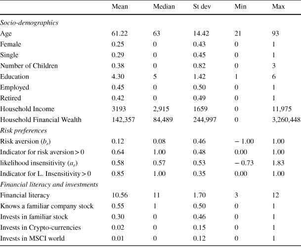
|
Mean |
Median |
St dev |
Min |
Max |
|
|---|---|---|---|---|---|
|
Socio-demographics |
|||||
|
Age |
61.22 |
63 |
14.42 |
21 |
93 |
|
Female |
0.25 |
0 |
0.43 |
0 |
1 |
|
Single |
0.29 |
0 |
0.45 |
0 |
1 |
|
Number of Children |
0.38 |
0 |
0.82 |
0 |
3 |
|
Education |
4.30 |
5 |
1.42 |
1 |
6 |
|
Employed |
0.45 |
0 |
0.50 |
0 |
1 |
|
Retired |
0.42 |
0 |
0.49 |
0 |
1 |
|
Household Income |
3193 |
2,915 |
1659 |
0 |
11,975 |
|
Household Financial Wealth |
142,357 |
84,489 |
244,997 |
0 |
3,260,448 |
|
Risk preferences |
|||||
|
Risk aversion (b r) |
0.12 |
0.08 |
0.46 |
− 1.00 |
1.00 |
|
Indicator for risk aversion > 0 |
0.64 |
1.00 |
0.48 |
0.00 |
1.00 |
|
likelihood insensitivity (a r) |
0.58 |
0.57 |
0.53 |
− 0.73 |
1.83 |
|
Indicator for L. Insensitivity > 0 |
0.85 |
1.00 |
0.35 |
0.00 |
1.00 |
|
Financial literacy and investments |
|||||
|
Financial literacy |
10.56 |
11 |
1.70 |
3 |
12 |
|
Knows a familiar company stock |
0.55 |
1 |
0.50 |
0 |
1 |
|
Invests in familiar stock |
0.30 |
0 |
0.46 |
0 |
1 |
|
Invests in Crypto-currencies |
0.02 |
0 |
0.15 |
0 |
1 |
|
Invests in MSCI world |
0.01 |
0 |
0.12 |
0 |
1 |
This table reports summary statistics of the socio-demographics, risk preferences, financial literacy and asset ownership of the investors in our sample. Sample size is n = 295 investors who owned bonds, mutual funds, individual stocks, or stock options as of 31 December 2016. Family income (monthly, after tax) and household financial wealth are measured in euros. The reference category for employment status is either unemployed or not actively seeking work (13%). Risk attitudes and investment in the familiar stock, crypto-currencies, and funds tracking the MSCI World index are measured in our ambiguity survey module (see text)
Appendix 2: Ambiguity attitudes of non-investors
Our survey was also given to a random sample of 304 non-investors, with 230 complete and valid responses (76%). Table 7 below displays summary statistics of the ambiguity attitudes of non-investors, index b and a. In the columns “Mean” and “Median”, stars (***, **, *) indicate whether the mean or median of the index is significantly different from the sample of investors in Table 1, at a significance level 10%, 5%, or 1%. More summary statistics of the non-investor sample and econometric analyses of their ambiguity attitudes are available in Online Appendix D.
Table 7 Descriptive Statistics of Ambiguity Measures–Non-Investor Sample
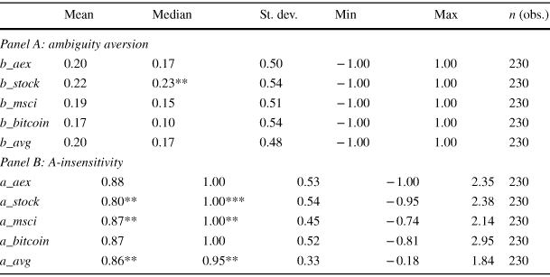
|
Mean |
Median |
St. dev. |
Min |
Max |
n (obs.) |
||||||
|---|---|---|---|---|---|---|---|---|---|---|---|
|
Panel A: ambiguity aversion |
|||||||||||
|
b_aex |
0.20 |
0.17 |
0.50 |
− 1.00 |
1.00 |
230 |
|||||
|
b_stock |
0.22 |
0.23** |
0.54 |
− 1.00 |
1.00 |
230 |
|||||
|
b_msci |
0.19 |
0.15 |
0.51 |
− 1.00 |
1.00 |
230 |
|||||
|
b_bitcoin |
0.17 |
0.10 |
0.54 |
− 1.00 |
1.00 |
230 |
|||||
|
b_avg |
0.20 |
0.17 |
0.48 |
− 1.00 |
1.00 |
230 |
|||||
|
Panel B: A-insensitivity |
|||||||||||
|
a_aex |
0.88 |
1.00 |
0.53 |
− 1.00 |
2.35 |
230 |
|||||
|
a_stock |
0.80** |
1.00*** |
0.54 |
− 0.95 |
2.38 |
230 |
|||||
|
a_msci |
0.87** |
1.00** |
0.45 |
− 0.74 |
2.14 |
230 |
|||||
|
a_bitcoin |
0.87 |
1.00 |
0.52 |
− 0.81 |
2.95 |
230 |
|||||
|
a_avg |
0.86** |
0.95** |
0.33 |
− 0.18 |
1.84 |
230 |
|||||
Panel A shows summary statistics for ambiguity attitudes regarding the local stock market index (b_aex), a familiar company stock (b_stock), the MSCI World stock index (b_msci), and Bitcoin (b_bitcoin), as well as the average of the four b-indexes (b_avg). Positive values of the b-index denote ambiguity aversion, and negative values indicate ambiguity seeking. The sample consists of n = 230 non-investors. Panel B shows summary statistics for a-insensitivity regarding the local stock market index (a_aex), a familiar company stock (a_stock), the MSCI World stock index (a_msci), and Bitcoin (a_bitcoin), as well as the average of the four a-indexes (a_avg). In the columns “Mean” and “Median”, stars (*, **, ***) indicate whether the mean and median of the index is significantly different from the sample of investors in Table 1, at 10%, 5%, or 1%


 Open access