INTRODUCTION
Although extinction is a recurrent evolutionary phenomenon, it does not proceed at the same pace at all times (Nakamura et al. Reference Nakamura, del Monte-Luna, Lluch-Belda and Lluch-Cota2013). Whilst a relatively low number of species usually become extinct during any given time span (background extinctions), there are periods during which a large proportion of biota is exterminated in a very short period in a geological timescale (mass extinctions) (Nakamura et al. Reference Nakamura, del Monte-Luna, Lluch-Belda and Lluch-Cota2013). In terrestrial groups, estimates of recent extinction rates are between 100- and 1000-times greater than the long-term global average derived from geological records (May et al. Reference May, Lawton, Stork, Lawton and May1995). In addition, the numbers of documented extinction are likely to be serious underestimates because most species are still unknown (Barnosky et al. Reference Barnosky, Matzke, Tomiya, Wongan, Quental, Marshall and Mersey2011; Joppa et al. Reference Joppa, Roberts and Pimm2011). Several researchers (e.g. May et al. Reference May, Lawton, Stork, Lawton and May1995; Joppa et al. Reference Joppa, Roberts and Pimm2011; Nakamura et al. Reference Nakamura, del Monte-Luna, Lluch-Belda and Lluch-Cota2013) thus suggest that humans are now causing the sixth mass extinction through co-opting resources, fragmenting habitats, introducing non-native species, polluting, killing species directly and inducing climate change (Barnosky et al. Reference Barnosky, Matzke, Tomiya, Wongan, Quental, Marshall and Mersey2011). In this context, there is an increasing need to find innovative tools to improve the effectiveness of biodiversity conservation.
One of the most common approaches in this sense is to model the presence or range of key species using remote data (He et al. Reference He, Bradley, Cord, Rocchini, Tuanmu, Schmidtlein, Turner, Wegmann and Pettorelli2015). These methods are widely used for a variety of reasons, including the high availability of remote sensing data (He et al. Reference He, Bradley, Cord, Rocchini, Tuanmu, Schmidtlein, Turner, Wegmann and Pettorelli2015) and because these can be used to predict how target species may respond to changes in climate or land use (Buckland & Elston Reference Buckland and Elston1993). Furthermore, predictions of species distribution models (SDMs) can sometimes reveal additional populations of threatened species (e.g. Alfaro-Saiz et al. Reference Alfaro-Saiz, García-González, del Río, Penas, Rodríguez and Alonso-Redondo2014; Fois et al. Reference Fois, Fenu, Cuena-Lombraña, Cogoni and Bacchetta2015) or guide the management of protected areas or other environments (e.g. Fois et al. Reference Fois, Cuena-Lombraña, Fenu, Cogoni and Bacchetta2016a; Kaky & Gilbert Reference Kaky and Gilbert2016). Increasingly, there is a need to use environmental data to identify those areas that might be candidate locations for species translocations (e.g. López-Tirado & Hidalgo Reference López-Tirado and Hidalgo2015; Fois et al. Reference Fois, Cuena-Lombraña, Fenu, Cogoni and Bacchetta2016a). However, despite their usefulness and large applicability, to our knowledge there are no examples of distribution models that use local extinctions in the Mediterranean territories. This is mainly due to a general lack of detailed information about where these extinctions have occurred (Greuter Reference Greuter1994; Domina et al. Reference Domina, Bazan, Campisi and Greuter2015).
Mediterranean islands provide a fascinating framework for studying the impact of human activity on biodiversity. With c. 10,000 islands and islets, 244 of which are inhabited (Pons et al. Reference Pons, Clarisó, Casademont and Arguimbau2013), the Mediterranean Basin encompasses one of the world's largest archipelagos (Pons et al. Reference Pons, Clarisó, Casademont and Arguimbau2013). Some eastern Mediterranean countries such as Greece (Iliadou et al. Reference Iliadou, Kallimanis, Dimopoulos and Panitsa2014) encompass a significant number of these islands; however, the western side includes the largest Mediterranean islands of Sicily, Sardinia and Corsica, as well as c. 1100 islets (Pons et al. Reference Pons, Clarisó, Casademont and Arguimbau2013).
For historical and geographical reasons, but also due to the particular biotic interactions among species, the particular Mediterranean insular conditions determine specific plant diversities and assemblages (Pons et al. Reference Pons, Clarisó, Casademont and Arguimbau2013). Plant endemism in Mediterranean islands often reaches high levels, generally comprising between 10% and 12% of the total vascular flora (e.g. Pons et al. Reference Pons, Clarisó, Casademont and Arguimbau2013; Fenu et al. Reference Fenu, Fois, Cañadas and Bacchetta2014). In particular, the plant endemism rate is generally higher in mountain ranges and in the satellite uninhabited islets of Sardinia, Corsica and Crete, where endemics represent c. 35–40% of the vascular flora (Iliadou et al. Reference Iliadou, Kallimanis, Dimopoulos and Panitsa2014; Fois et al. Reference Fois, Fenu and Bacchetta2016b).
Plant diversity in Mediterranean insular territories shares its heritage with several human activities that have had profound, often negative consequences for plant distributions and dynamics (Lavergne et al. Reference Lavergne, Thuiller, Molina and Debussche2005; Pungetti et al. Reference Pungetti, Marini, Vogiatzakis, Pungetti and Mannion2008). In the Mediterranean Basin, climatic anomalies (e.g. López-Tirado & Hidalgo Reference López-Tirado and Hidalgo2015; Kaky & Gilbert Reference Kaky and Gilbert2016) and human-related factors, such as human trampling and land use change (e.g. Lavergne et al. Reference Lavergne, Thuiller, Molina and Debussche2005; Fenu et al. Reference Fenu, Cogoni, Ulian and Bacchetta2013), have been identified as important drivers of local extinctions or population decreases in narrowly distributed plants; however, several data gaps still exist (Greuter Reference Greuter1994; Domina et al. Reference Domina, Bazan, Campisi and Greuter2015).
This study focused on local extinctions of vascular plants that occurred since 1960 on the island of Sardinia. An experimental approach was possible due to the unusually long-term documented investigations of the island's flora. Indeed, many documents on regional flora were published when environmental conditions were different; this has allowed authors to previously discuss the local extinctions of specific areas such as the small satellite islets (Bocchieri Reference Bocchieri1998) and the north-western part of Sardinia (Bagella & Urbani Reference Bagella and Urbani2006). The main aims of this study were: (1) to identify extinction locations of plant species of concern in Sardinia; (2) to investigate how important each considered variable was in determining local extinctions by measuring the relative influence of anthropogenic factors in relation to ecological constraints; and (3) to explore the extinction pattern and to identify, by a novel application of SDMs, areas where plant extinctions may potentially occur. The utility of this approach was tested for localizing and mapping areas where anthropogenic and ecological drivers of local extinctions were most influential and where further investigations of extinction threats could be focused.
METHODS
Study area
Sardinia and its c. 399 satellite small islands cover 24,090 km2 with a coastline of c. 1900 km. The island is characterized by complex orography with plain, hilly and mountainous landscapes on different geological substrates. The climate it has is typically Mediterranean, with dry and hot summers and relatively rainy and mild winters, with a temperate bioclimate only on the higher summits. These traits, in conjunction with its prolonged isolation, are the main factors that promoted the speciation of endemic plants (Cañadas et al. Reference Cañadas, Fenu, Peñas, Lorite, Mattana and Bacchetta2014). The subsequent high proportion of endemic taxa (c. 13% of the entire flora) (Fenu et al. Reference Fenu, Fois, Cañadas and Bacchetta2014) considerably increases up to c. 35% on mountain peaks and uninhabited islets (Cañadas et al. Reference Cañadas, Fenu, Peñas, Lorite, Mattana and Bacchetta2014; Fois et al. Reference Fois, Fenu and Bacchetta2016b).
Sardinia is underpopulated compared to other Italian (and European) regions: it has a demographic density of 66 inhabitants per km2, compared with an average of 194 inhabitants per km2 in the whole of Italy (ISTAT 2001). Nonetheless, the long presence of human habitation has been pivotal to shaping Sardinia's landscape and its plant diversity (Pungetti et al. Reference Pungetti, Marini, Vogiatzakis, Pungetti and Mannion2008). Plant extinctions in Sardinia, as well as in the entire Mediterranean region, are bound to have occurred in historical times with the massive development of agriculture and the related significant environmental transformations. In particular, the island has gone from the wilderness of its original Mediterranean habitats to an agricultural landscape with wheat fields in the plains, vineyards on the slopes and pastoral land in the highlands (Pungetti et al. Reference Pungetti, Marini, Vogiatzakis, Pungetti and Mannion2008). As on many other Mediterranean islands, industrial, seasonal (summertime) and local (coastal) tourist activities have also grown rapidly in recent decades in lowland plains and coastal areas (Pungetti et al. Reference Pungetti, Marini, Vogiatzakis, Pungetti and Mannion2008).
Local extinctions and occurrence data
The study focused on a selected group of vascular plants with local biogeographical and/or conservation interest in Sardinia. In particular, plants of biogeographical interest were those endemic to the Sardo-Corsican biogeographical province (Fenu et al. Reference Fenu, Fois, Cañadas and Bacchetta2014) and/or those plants that, from their geographical disjunction, are proved to be ecologically and/or genetically isolated (Arrigoni Reference Arrigoni1983). Plants of conservation interest were those listed at least as ‘Endangered’ at a regional or global level on the International Union for Conservation of Nature (IUCN) database (IUCN 2016) and/or listed in international protection regulations (see Fenu et al. Reference Fenu, Fois, Cogoni, Porceddu, Pinna, Cuena-Lombraña, Nebot, Sulis, Picciau, Santo, Murru, Orrù and Bacchetta2015 for details).
Information about both present occurrences and extinction localities was obtained from herbarium collections (University of Cagliari, University of Catania, Natural History Museum of Florence, Museum Herbarium of the ‘Sapienza’ University of Rome, University of Sassari (Faculty of Sciences), University of Sassari (Faculty of Pharmacy) and University of Turin) and available literature and was confirmed and implemented by the unpublished field survey records of the authors. While the creation of the occurrences dataset consisted of updating datasets used in previous studies (e.g. Fenu et al. Reference Fenu, Fois, Cañadas and Bacchetta2014; Fois et al. Reference Fois, Fenu, Cuena-Lombraña, Cogoni and Bacchetta2015, Reference Fois, Fenu and Bacchetta2016b), the extinction localities dataset was constructed ad hoc for this research. All reported extinctions of local flora (e.g. Bacchetta Reference Bacchetta2006; Pisanu et al. Reference Pisanu, Farris, Caria, Filigheddu, Urbani and Bagella2014) and all research on floristic changes (e.g. Bocchieri Reference Bocchieri1998; Bagella & Urbani Reference Bagella and Urbani2006) and conservation status assessments (e.g. Fenu et al. Reference Fenu, Mattana and Bacchetta2012; Fois et al. Reference Fois, Cuena-Lombraña, Fenu, Cogoni and Bacchetta2016a) were taken into account. Further extinctions occurring during the last 10 years were directly recorded by the authors through revisiting localities with reports of threatened plants. Using the framework of specific demographic studies (e.g. Morris & Doak Reference Morris and Doak2002), localities with fewer than 20 reproductive individuals were considered to be sites of extinction and were included in these analyses. All distribution data were recorded within a grid of 1 × 1 km in a Geographic Information System environment (Quantum GIS Development Team 2014). In the final database, the plants were categorized according to Raunkiaer's lifeform classification system (Raunkiaer Reference Raunkiaer1934), which is based on the place of the plant's growth-point during seasons with adverse conditions, reflecting the adaptation of plants to surviving in unfavourable seasons (cold or dry seasons) and is correlated with growth forms: therophytes (annual plant species), hemicryptophytes (perennial forbs and grasses), geophytes (perennial plants with bulbs, corms or rhizomes), chamaephytes (semi-shrubs) and nanophanerophytes/phanerophytes (shrubs and trees).
Because altitude was one, if not the main factor related to the distribution of several plant species in Sardinia (e.g. Cañadas et al. Reference Cañadas, Fenu, Peñas, Lorite, Mattana and Bacchetta2014; Fois et al. Reference Fois, Fenu, Cuena-Lombraña, Cogoni and Bacchetta2015, Reference Fois, Fenu and Bacchetta2016b), another subdivision was implemented according to altitudinal range, obtained using extrapolated mean values per 1-km2 grid cell: coastal (0–150 metres above sea level (m asl)), plains and hilly (10–800 m asl), mountainous (>800 m asl) or widespread (altitudinal range >1000 m asl).
Ecological and anthropogenic factors
Data used as explanatory variables in the extinction models were subdivided into two categories: ecological and anthropogenic variables (Table 1). The first group included two monthly mean climatic datasets (Bio7 and Bio15) for current conditions (from the years of c. 1950 to 2000) and three geomorphological variables (Elev (elevation), Slope (morphological steepness) and Lith (lithology)), which were extrapolated using a digital terrain model and a simplified geological map of Sardinia (Table 1) (Fenu et al. Reference Fenu, Fois, Cañadas and Bacchetta2014). The anthropogenic factors were compiled from a free worldwide raster dataset called Human Influence Index (HII) (WCS & CIESIN 2005), the total length in metres of streets per grid cell (‘street’) and the number of fires that occurred over a 9-year period (2005–2013; ‘fires’). All variables were converted to raster format at the same 1-km2 resolution of species data.
Table 1 List of variables subdivided into ecological (E) or anthropogenic (A) and their respective sources. Problems related to collinearity were avoided by removing factors with variance inflation factor (VIF) values of >5. DTM = digital terrain model; Elev = elevation; HII = Human Influence Index; Lith = lithology; Slope = morphological steepness.

Multicollinearity problems were tested by computing variance inflation factors (VIFs) (Marquardt Reference Marquardt1970), which measure how strongly each predictor can be explained by the rest of the predictors and are based on the square of the multiple correlation coefficient (R2) resulting from regressing the predictor variable against all other predictor variables (Naimi & Araújo Reference Naimi and Araújo2016). As a rule of thumb, a VIF of >10 signals that the model has a collinearity problem (Chatterjee & Hadi Reference Chatterjee and Hadi2006). We used a stepwise procedure, implemented through the ‘sdm’ package (Naimi & Araújo Reference Naimi and Araújo2016) in the R environment (version 3.1.1) (R Development Core Team Reference Core Team2014) in order to remove all variables with VIFs of >5, which was imposed as a precautionary threshold (Table 1).
Evaluation of variable importance
The effect of each independent variable was tested by means of generalized linear models (GLMs) using the logistic (0: extant locations; 1: extinct locations) as a link function and the binomial as an error distribution (Carrete et al. Reference Carrete, Grande, Tella, Sánchez-Zapata, Donázar, Díaz-Delgado and Romo2007). We performed a hierarchical partitioning analysis (package ‘hier.part’) (Walsh & MacNally Reference Walsh and MacNally2013) in the R environment (version 3.1.1) (R Development Core Team Reference Core Team2014) in order to estimate the independent effect of each factor on determining local extinctions. This process involved computing the increase in the fit (measured as deviance explained) of all models with a particular variable compared with the equivalent model without that variable. In this way, multicollinearity problems that are effectively ignored by using any one-model technique are likely to be alleviated (MacNally Reference MacNally2000). The size of the individual effect of each variable (percentage of independent effect) was used as a criterion for ranking and deriving conservation extinction risks. We assumed only variables with an independent effect of >10% (MacNally Reference MacNally2000) as possible causes of extinctions. Analyses were repeated for each taxon and then averaged according to lifeform and altitudinal range classifications. If no variables satisfied this criterion, local extinctions were considered stochastic. After selecting the most important factors driving the extinctions of each taxon, the respective range values of occurrences and extinctions were compared.
Procedures, evaluation and ensemble of distribution models
The same binary form of extinct (1) and extant (0) records was applied in order to predict potential areas where local extinctions may occur. Species with only one extinction event and/or fewer than three occurrence records were excluded from these analyses due to their low reliability (van Proosdij et al. Reference van Proosdij, Sosef, Wieringa and Raes2015). In addition, only extinction causes that were highlighted according to their variable importance (independent effect of >10%) were employed in each species-specific model (Table S1) (available online).
GLM and random forest (RF) presence–absence methods were used to model plant extinctions as the basis of a final mean ensemble method (Araújo & New Reference Araújo and New2007; Marmion et al. Reference Marmion, Parviainen, Luoto, Heikkinen and Thuiller2009). These techniques, which are widely used to model species distributions and are capable of modelling nonlinear functions (Franklin Reference Franklin2010), were implemented by using the R ‘sdm’ package, an integrated framework that enables multiple modelling techniques to be fitted and compared simultaneously (Naimi & Araújo Reference Naimi and Araújo2016). The settings that are implemented by the ‘sdm’ package were applied by default. In particular, GLMs with logistic link functions and RF models with 500 trees were used.
For each model, we used 10-fold cross-validations in order to give a more robust estimate of predictive performance (Elith et al. Reference Elith, Phillips, Hastie, Dudík, Chee and Yates2011). For each cross-validation iteration, 70% and 30% of the data were randomly selected for use as training and testing datasets, respectively (Elith et al. Reference Elith, Phillips, Hastie, Dudík, Chee and Yates2011). Model performance was determined by calculating the area under the curve (AUC) of a receiver operating characteristic plot (Fielding & Bell Reference Fielding and Bell1997) and the true skill statistic (TSS) (Allouche et al. Reference Allouche, Tsoar and Kadmon2006) using the model validation dataset. Results were averaged over 10 replicates per modelling technique.
The final extinction model for each species was calculated as the mean value of the outputs of all single runs. This consensus approach has recently been applied in broad-scale conservation studies and is based on the idea that different predictions are copies of possible states of real distributions and that their ensemble will result in a more accurate prediction (Marmion et al. Reference Marmion, Parviainen, Luoto, Heikkinen and Thuiller2009). In addition, this allows a comparison of the methods’ predictive abilities and a quantification of uncertainties deriving from the choice of the modelling approach (Marmion et al. Reference Marmion, Parviainen, Luoto, Heikkinen and Thuiller2009; Naimi & Araújo Reference Naimi and Araújo2016).
The type of output provided varied in relation to the modelling technique used. The ‘sdm’ package enabled different predictions to be standardized in a continuous index of probability, ranging from 0 (low probability of extinction) to 1 (high probability of extinction). The outputs used for the ensemble were at least satisfactorily (AUC >0.7 and TSS >0.3) (Heikkinen et al. Reference Heikkinen, Marmion and Luoto2012) predicted by the models.
The final result was thus obtained by merging all species-specific outputs (if satisfactory) with the ‘merge’ function of raster R package (Hijmans et al. Reference Hijmans, van Etten, Mattiuzzi, Sumner, Greenberg, Lamigueiro, Bevan, Racine and Shortridge2015) and plotted in a GIS environment (Quantum GIS Development Team 2014) in order to graphically depict the areas of conservation interest.
RESULTS
A total of 62 vascular plant species (for 190 extinction events and 2357 occurrence records) were analysed; 39 of these species were considered to have both conservation and biogeographical interest, while only 10 and 13 plant species were considered to have only biogeographical or conservation interest, respectively. The 62 plant species included 10 therophytes, 19 hemicryptophytes, nine geophytes, 14 chamaephytes and 10 nanophanerophytes/phanerophytes. Altitudinally, the plant species were subdivided into coastal (18 species), plains and hilly (12 species), mountainous (four species) and widespread (14 species) (Table S2).
Evaluation of variable importance
Both ecological and anthropogenic factors explained the local extinctions of 34 plant species, whereas in only 14 and five cases, respectively, did ecological or anthropogenic factors exclusively explain extinctions. Six cases were assumed to be stochastic (Table S2).
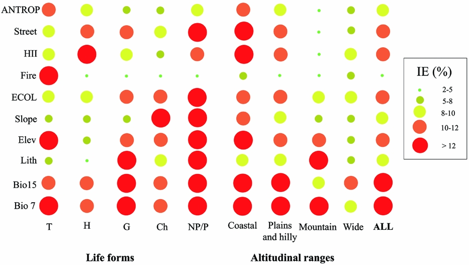
Ecological factors fairly equally influenced extinctions among lifeforms and altitudinal ranges. The only exceptions were plants with a wide altitudinal range, the influence of which was generally considered to be stochastic (Fig. 1). Otherwise, the influence of anthropogenic factors was greater for therophytes, chamaephytes and nanophanerophytes/phanerophytes, especially in coastal and plains/hilly localities (Fig. 1).

Figure 1 Scatterplots of the percentage of independent effects (IE%) of each variable (Bio7 = temperature annual range; Bio15 = precipitation seasonality; Lith = lithology; Elev = elevation; Slope = morphological steepness; Fire = number of fires that occurred from 2005 to 2013; HII = Human Influence Index; Street = metres of streets per grid; see Table 1 for further details) and the means of the ecological (ECOL) and anthropogenic (ANTROP) groups. Values were the average of each model obtained from the 62 vascular plants analysed. These were considered all together (ALL) and also subdivided according to altitudinal ranges and lifeforms proposed by Raunkiaer (Reference Raunkiaer1934) (T = therophytes; H = hemicryptophytes; G = geophytes; Ch = chamaephytes; NP/P = nanophanerophytes/phanerophytes; see Table S2 for further details).
If all analysed plant species are considered together, ecological factors (in particular temperature annual range and precipitation seasonality) explained local extinctions more than anthropogenic factors (Fig. 1).
Model evaluation and ensemble forecasting
Extinction distribution models were implemented for 101 extinction localities of 32 plant species. Model performances were generally high in terms both of AUC and TSS values (Fig. 2). Nonetheless, the ensemble of RF and GLM algorithms was not used in nine cases because one of these two approaches did not satisfy the AUC (>0.7) and/or TSS (>0.3) thresholds; in only two cases did neither algorithm satisfy the criteria (Table S3).
Figure 2 Boxplots of the model performance measures (area under the curve (AUC) and true skill statistic (TSS)) of both techniques used (random forest (RF) and generalized linear model (GLM)).
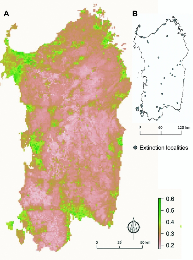
The final map, which was obtained by merging the 30 species-specific outputs, highlighted the areas where drivers of plant extinctions should be more influential. The probability of extinction was higher (>0.4) along the coast and in plains areas (Fig. 3).

Figure 3 Average map of 101 local extinction cases per 32 singularly modelled plant species (a). Values from 0 to 1 measured the probabilities of extinction across all of the Sardinian territory. Localities of extinctions used are reported on the right (b).
DISCUSSION
Despite the importance of disentangling the causes of recent extinctions, researchers have faced many difficulties in finding correlations between extinction events and anthropogenic/ecological factors. This is mainly due to the unavailability of historical information on plant occurrences and/or extinctions (Greuter Reference Greuter1994) and because extinctions are sometimes caused by stochastic events and/or to the combined effects of many factors (Renton et al. Reference Renton, Shackelford and Standish2014). For these reasons, large-scale research on extinctions is barely feasible, but similar studies can be carried out for small and well-delineated areas, such as Mediterranean islands, which are historically well known from plant diversity and floristic viewpoints. Nonetheless, we argue that the results obtained for our specific case could reflect the extinction patterns of similar contexts, such as other coastal areas of the Mediterranean or other regions with high endemicity combined with long histories of human-induced transformations.
According to other studies in the Mediterranean context (e.g. Lavergne et al. Reference Lavergne, Thuiller, Molina and Debussche2005; Fenu et al. Reference Fenu, Cogoni, Ulian and Bacchetta2013), both anthropogenic and environmental variables explain extinctions, and they also explain the distributions of endangered coastal plant species in Sardinia. Although ecological factors generally explained local extinctions more than anthropogenic factors, the independent effects of each factor considerably varied between lifeforms and altitude ranges. Such differences confirmed the necessity for supporting general overviews with detailed studies, since species- or habitat-specific results are sometimes in contrast with the general trend.
The effect of anthropogenic factors was less strong for geophyte and chamaephyte extinctions than for therophytes, hemicryptophytes and nanophanerophytes/phanerophytes. Geophytes and chamaephytes have previously been recognized as two of the plant forms that are most resistant to fires, trampling and grazing (Pignatti et al. Reference Pignatti, Pignatti and Ladd2002). Although the degree of sensitivity to anthropogenic factors was difficult to determine in our analyses, the independent effects of each variable implicitly suggest different degrees of sensitivity between lifeforms. The HII, which is a sum of many anthropogenic factors, was likely to be a finer measure of even low-intensity disturbances than the total length of streets per grid (Fig. 1 and Table 1; ‘street’), which accounted for a more destructive level of disturbance. This could explain why even a low-intensity disturbance, such as human trampling, was an influential factor for many coastal endangered hemicryptophytes, such as Anchusa crispa (Bacchetta et al. Reference Bacchetta, Coppi, Pontecorvo and Selvi2008) and Astragalus maritimus (Bacchetta et al. Reference Bacchetta, Fenu, Mattana and Pontecorvo2011), while coastal nanophanerophytes and phanerophytes were only influenced by more intense disturbances that were often connected to the development of infrastructure (Tzanopoulos et al. Reference Tzanopoulos, Mitchley and Pantis2005). The frequency of fires (Fig. 1 and Table 1; ‘fires’) only explained extinction events for therophytes. Although covers of annual plant communities generally increase with human disturbance (Pignatti et al. Reference Pignatti, Pignatti and Ladd2002), Mediterranean endemic and specialist therophytes are likely to have a lower tolerance to competition than endemic and specialist perennial lifeforms (Imbert et al. Reference Imbert, Youssef, Carbonell and Baumel2011; Fenu et al. Reference Fenu, Cogoni, Ulian and Bacchetta2013). This competition is particularly important for annual species in soil seed banks, where burning events often cause a reduction in seed bank diversity, benefiting perennial lifeforms and widespread and/or pioneer plants (Torres et al. Reference Torres, Urbieta and Moreno2012). Fires could have a particular negative influence on less competitive species, such as the endemic and specialist therophytes.
The influence of ecological factors, which are often complementary to and/or consequences of anthropogenic activities (Lavergne et al. Reference Lavergne, Thuiller, Molina and Debussche2005; Renton et al. Reference Renton, Shackelford and Standish2014), was similar among species’ altitudinal ranges, with the exception of wide-ranging species. According to previous research (e.g. Imbert et al. Reference Imbert, Youssef, Carbonell and Baumel2011; Renton et al. Reference Renton, Shackelford and Standish2014; Kaky & Gilbert Reference Kaky and Gilbert2016), plants with a wide distribution and ecological range are less prone to suffer as a result of climatic changes than those that occur only in specific environments, such as coasts and Mediterranean mountains. This discussion regarding species with narrow ecological requirements could also be applied in order to explain the influence of lithology, which is especially characteristic in geophytes, including orchids (Djordjević et al. Reference Djordjević, Tsiftsis, Lakušić and Stevanović2014) and many perennial endemics such as taxa belonging to the genus Ribes in Sardinia (Fenu et al. Reference Fenu, Mattana and Bacchetta2012).
The areas highlighted by averaging all modelled extinction cases were characterized by land use change from semi-natural into urbanized landscapes that has occurred in recent decades (Zoppi & Lai Reference Zoppi and Lai2012). This was mainly a consequence of industrial settlements (e.g. in the north-western and south-western coasts of Porto Torres and Portoscuso, respectively) and increasing tourism development along the rest of the coast. Otherwise, most similar neighbouring environments were considered important areas for plant conservation owing to their high numbers of endemic and/or threatened plant species (Fenu et al. Reference Fenu, Fois, Cañadas and Bacchetta2014; Fois et al. Reference Fois, Fenu and Bacchetta2016b). This result aligned with our expectations due to the implicit ecological information contained in the modelled extinction localities of the analysed endemic and endangered species.
The idea behind this research was to treat occurrence data in an experimental way. Indeed, the common usage of presence data in SDMs was in this case replaced by extinction occurrences. Therefore, this approach could be defined as an extinction (and not species) distribution model that underscored potential threatened areas instead of potential niches. Therefore, the species-specific results that are usually obtained by environmental modelling could be extended in this case to more generalized results for potential areas of extinctions and thus threats, which refer not only to each singular specific case, but also to all taxa with a similar pattern and ecology. This potential is strengthened by averaging many cases that occurred in a diversified environment (from coastal to mountainous areas and from rural to semi-urban areas). To our knowledge, no scholars have used a similar methodological approach to that which was used in this research; hence, at this stage, comparisons with our results are not possible.
Although correlation does not imply causation, our stepwise procedure of investigating drivers of extinctions has suggested further insights regarding how and where extinctions may occur in Sardinia. Instead of representing the mere pattern of recorded extinctions, our resulting map also allowed us to highlight those vulnerable areas that probably have been insufficiently investigated and thus where further populations that are extinct or at the brink of extinction could perhaps be found. In other words, the threatened areas identified by our study should not simply be considered to be loser zones. Conversely, these should be considered areas in which much more interesting work, such as ecological analyses and conservation activities, could be focused.
Because part of our analysis used an experimental approach, we have a special interest in sharing the results of this research in order to compare our results with those of different species and/or species in other environmental conditions. As information about even recent extinctions is seldom reported in the literature, only further investigations and comparisons can enhance the current state of the art regarding the main reasons underlying recent extinctions, which are often based on suppositions and underestimations (Barnosky et al. Reference Barnosky, Matzke, Tomiya, Wongan, Quental, Marshall and Mersey2011; Joppa et al. Reference Joppa, Roberts and Pimm2011). Furthermore, this research provides a general perspective that should be implemented through more focused investigations of each analysed species. Other researchers are thus invited to take into account our general and species-specific results that are reported in the supplementary materials in order to analyse and compare them with their own study cases.
ACKNOWLEDGEMENTS
We are grateful to Angelino Congiu, Giacomo Calvia and Giuliano Mereu for providing information on local extinctions and two anonymous reviewers for their constructive comments.
Supplementary Material
For supplementary material accompanying this paper, visit https://doi.org/10.1017/S0376892917000108