Introduction
Increasing anthropogenic pressures such as land-use changes have led to a growing loss of biodiversity and changes in the functioning of ecosystems (e.g., Butchart et al. Reference Butchart, Walpole, Collen, van Strien, Scharlemann, Almond and Baillie2010), with important consequences for the social and economic benefits involved, provided typically free of charge (e.g., MEA 2005, IPBES Reference Fischer, Rounsevell, Torre-Marin Rando, Mader, Church, Elbakidze and Elias2018). Protected areas have long been the mainstay of biodiversity conservation (e.g., Gray et al. Reference Gray, Hill, Newbold, Hudson, Borger, Contu and Hoskins2016). The Natura 2000 network in Europe represents one of the world’s most ambitious regulatory frameworks regarding biodiversity conservation (Bastian Reference Bastian2013). Natura 2000 sites have mainly been designated according to ecological criteria to meet specific conservation objectives (Bastian Reference Bastian2013, Kukkala et al. Reference Kukkala, Arponen, Maiorano, Moilanen, Thuiller, Toivonen and Zupan2016).
However, the implementation of protected areas is not always ‘peaceful’ (Baelde Reference Baelde2005). Most conservation programmes require some form of zoning. Depending on their geographical distribution, biodiversity hotspots are often located in places occupied by local communities where socioeconomic activities take place. The designation of protected areas in these locations has received considerable criticism due to the lack of a systematic approach in practical conservation planning or planning new reserves in places that do not contribute significantly to the preservation of biodiversity, among other factors (e.g., Margules & Pressey Reference Margules and Pressey2000, Fuller et al. Reference Fuller, McDonald-Madden, Wilson, Carwardine, Grantham, Watson and Klein2010). Regulations underlying protected areas aimed at the conservation of ecosystems are usually applied in a standard manner (e.g., Santos et al. Reference Santos, Ring, Antunes and Clemente2012), regardless of the level of benefits provided, the ecosystem baseline conditions or the cost of conserving those areas. Other criticisms point out the limitations that protected areas impose on local populations, raising questions about their fairness, especially in cases where local biodiversity conservation yields global benefits (Perrings & Gadgil Reference Perrings, Gadgil, Kaul, Conceição, Le Goulven and Mendoza2003).
To promote a more equitable and cost-effective implementation of conservation measures, different ecosystem features (e.g., species distribution or carbon sequestration), economic costs (e.g., opportunity or transaction costs), policy instruments (e.g., payments for ecosystem services or agro-environmental measures (AEMs)) and analytical tools (e.g., multi-criteria analysis) have been developed using spatial planning approaches (e.g., Schwartz et al. Reference Schwartz, Cook, Pressey, Pullin, Runge, Salafsky, Sutherland and Williamson2017). Spatial targeting has helped not only to better account for the benefits provided by existing policy implementation, but also to ensure that policy interventions are more efficient through ex ante evaluation (Wunder et al. Reference Wunder, Brouwer, Engel, Ezzine-de-Blas, Muradian, Pacual and Pinto2018). However, challenges remain regarding finding appropriate tools that allow for the full integration of different types of ecological and economic data and information (e.g., Wätzold et al. Reference Wätzold, Drechsler, Armstrong, Baumgärtner, Grimm, Huth and Perrings2006, Schaefer et al. Reference Schaefer, Goldman, Bartuska, Sutton-Grier and Lubchenco2015). No standard approach exists that can be applied to all situations. Depending on context and objectives, different models may be available or may have to be developed in order to address the sustainable management of ecosystems and associated biodiversity.
In this study, we implement Marxan with Zones (MARZONE) (Watts et al. Reference Watts, Ball, Stewart, Klein, Wilson, Steinback and Lourival2009) to evaluate current and inform future spatial planning of appropriate AEMs and silvo-environmental measures (SEMs) and corresponding conservation targets inside and outside of existing protected areas in the Montado ecosystem in south Europe. Considering four different AEMs and SEMs, a comprehensive integrated assessment of the trade-offs between biodiversity conservation and its financial and economic costs is provided at a regional scale. MARZONE is used to incorporate different conservation management measures, features and costs, and hence assess: (1) how existing planning tools can be improved to prioritize management options such as AEMs and SEMs within the Montado landscape; (2) the cost-effectiveness of programmes of measures; and (3) the extent to which current protection networks incorporate relevant biodiversity hotspots. To the best of our knowledge, this is the first attempt to use MARZONE to spatially allocate AEMs and SEMs within a biodiversity hotspot region (Supplementary Information S1, available online). New in this study is that a distinction is made between the financial compensation paid to landowners adopting the AEMs and SEMs and the broader economic costs of associated land-use changes. Of particular interest is also setting up the spatial model in a collaborative manner with policy-makers, decision-makers and other stakeholders in order to improve the effective communication of the outcomes (Videira et al. Reference Videira, Antunes, Santos, Gray, Paolisso, Jordan and Gray2017). To this end, we map the relevant ecological and economic parameters in the study area to assess potential trade-offs when aiming to protect the Montado ecosystem, and we include these parameter values in the Marxan spatial planning tool to evaluate where priority areas are found. Based on the obtained results, we identify the areas that optimize current and guide future conservation planning.
Case study area
This study was conducted in the southeast of Portugal, covering a total area of 2860 km2 with a low population density (Fig. 1). The topography of the area is relatively flat, with slopes of between 0% and 5%. The climate is dry, with an average annual precipitation of c. 500 mm (PBH Guadiana 2001). The study site was selected due to the high conservation value of the Montado ecosystem in the area (e.g., Pinto-Correia et al. Reference Pinto-Correia, Guiomar, Ferraz-de-Oliveira, Sales-Baptista, Rabaça, Godinho and Ribeiro2018). In recognition of its important value, the Montado is protected under several European laws and national regulations, including Natura 2000. The Montado is a multifunctional, human-shaped ecosystem resulting from centuries of human–nature interactions. It is highly dependent on land-use and human activities (Bugalho et al. Reference Bugalho, Caldeira, Pereira, Aronson and Pausas2011, Sá-Sousa Reference Sá-Sousa2014). Therefore, prohibiting development is not sufficient to conserve the Montado ecosystem.
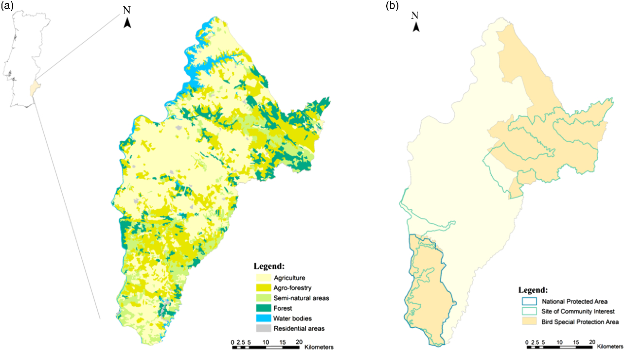
Fig. 1. Location of the case study area in Portugal: (a) main land uses; (b) protected areas (sources: CORINE Land Cover 2006 and ICNF).
The study area comprises multifunctional landscapes including agricultural sites, urban settlements, national protected areas and Natura 2000 sites. An ecological corridor is planned in the central part of the case study area in order to reduce the negative impacts of habitat fragmentation, linking the north-eastern and south-western protected areas (Magalhães et al. Reference Magalhães, Abreu, Lousã, Cortez, Conceição and Raichande2007). The most common agricultural activities involve cereal crops, including wheat, cork, olive oil, wine and extensive livestock grazing (Fragoso et al. Reference Fragoso, Marques, Lucas, Martins and Jorge2011, Sá-Sousa Reference Sá-Sousa2014).
The typical Montado landscape in the study area provides a wide range of habitats, from open savannas (hereafter ‘open Montado’) to forests presenting a scattered tree cover of 60–100 trees per hectare (hereafter ‘dense Montado’) (e.g., Simonson et al. Reference Simonson, Allen, Parham, Basto-Santos and Hotham2018). These multifunctional ecosystems provide habitats for globally threatened species, including the great bustard (Otis tarda) and the red kite (Milvus milvus), and they are an important wintering ground for migratory birds such as the little bustard (Tetrax tetrax). Biodiversity trends in the Montado ecosystem in the case study area are described in more detail in Simonson et al. (Reference Simonson, Allen, Parham, Basto-Santos and Hotham2018).
The use of traditional agro-pastoral and extensive oak woods in the region has been threatened by both natural (e.g., high frequency of wildfires) and anthropogenic driving forces (e.g., agricultural intensification and increasing land abandonment) (Acácio et al. Reference Acácio, Holmgren, Moreira and Mohren2010, Pinto-Correia & Godinho Reference Pinto-Correia, Godinho, Ortiz-Miranda, Moragues-Faus and Arnalte-Alegre2013, Pinto-Correia et al. Reference Pinto-Correia, Guiomar, Ferraz-de-Oliveira, Sales-Baptista, Rabaça, Godinho and Ribeiro2018, Soares et al. Reference Soares, Príncipe, Köbel, Nunes, Branquinho and Pinho2018), leading to a loss of Montado area at a rate of c. 0.14% per year (Godinho et al. Reference Godinho, Guiomar, Machado, Santos, Sa-Sousa, Fernandes, Neves and Pinto-Correia2016). Despite the existing protected areas, the poor management of the traditional multifunctional oak system is expected to lead to more single-function patches and the loss of landscape values and resources in the future.
Methodological approach
Spatial model
When identifying potential priority areas for protection, there are two main approaches that dominate the literature (Ando et al. 1998). The minimum set approach aims to minimize a loss function (e.g., the cost of selected sites) based on established conservation targets, while the maximum coverage approach aims to maximize the achievement of conservation targets. Within this scope, several tools and software programs have been developed. Answering to the minimum set approach, Marxan is the most widely applied strategic conservation planning tool (Possingham et al. Reference Possingham, Moilanen, Wilson, Moilanen, Wilson and Possingham2000, Ball et al. Reference Ball, Possingham, Watts, Moilanen, Wilson and Possingham2009). MARZONE is a land-use zoning tool based on Marxan (Watts et al. Reference Watts, Klein, Stewart, Ball and Possingham2008a, Reference Watts, Ball, Stewart, Klein, Wilson, Steinback and Lourival2009). Compared to Marxan, MARZONE allows for the incorporation of multiple conservation measures and costs, introducing more flexibility in the spatial analysis (Watts et al. Reference Watts, Ball, Stewart, Klein, Wilson, Steinback and Lourival2009).
One of the distinguishing features is that MARZONE can assign different conservation measures (zones) to land planning units (PUs), while optimizing the relationship between the achievement of conservation targets and the costs of the possible measures to reach the conservation targets (Ball & Possingham Reference Ball and Possingham2000, Ball et al. Reference Ball, Possingham, Watts, Moilanen, Wilson and Possingham2009). This cost-effective selection is based on so-called simulated annealing (i.e., a linear integer programming procedure that can be combined with an iterative improvement algorithm to find multiple (near-optimal) solutions) (Kirkpatrick et al. Reference Kirkpatrick, Gelatt and Vecchi1983, Ball et al. Reference Ball, Possingham, Watts, Moilanen, Wilson and Possingham2009). The mathematical representation of the objective function is given in Eq. (1) (Watts et al. Reference Watts, Klein, Stewart, Ball and Possingham2008a):
 $$Min\left[ {\mathop \sum \limits{_P}{_U} Cost + BLM\mathop \sum \limits{_P}{_U} BL + FPF\mathop \sum \limits{_P}{_U} Penalty} \right]$$
where the score for the following three components is minimized across the PUs: (1) the Cost of selecting a PU (i.e., the opportunity cost of its land use); (2) the boundary length (BL), which provides an indication of the degree of connectivity between the PUs, weighted by a constant boundary length multiplier (BLM) – the latter equals the importance attached to boundary length compared to the cost of the zone configuration; and (3) a Penalty for not representing every conservation feature in every PU, also multiplied by a weighting factor called the feature penalty factor (FPF) in order to determine the relative importance for satisfying a particular feature’s target.
MARZONE has mostly been applied to optimize terrestrial and marine conservation policies (e.g., Wilson et al. Reference Wilson, Meijaard, Drummond, Grantham, Boitani, Catullo and Christie2010, Peckett Reference Peckett2015, Law et al. Reference Law, Bryan, Meijaard, Mallawaarachchi, Struebig, Watts and Wilson2017), and more recently also to optimize freshwater ecosystem conservation in catchments (e.g., Parker et al. Reference Parker, Truscott, Harpur and Murphy2015, Hermoso et al. Reference Hermoso, Cattarino, Linke and Kennard2018). Supplementary Fig. S1 and Table S1 present an extensive overview of 58 studies that were identified in the literature using MARZONE as a spatial conservation tool.
Practical steps
The steps in the spatial analysis using MARZONE are defined in Supplementary Table S2, including the data and information used in each step to build the spatial input files for MARZONE. The spatially explicit mathematical programming software consistently links fine-grain issues (species abundance and distribution) to broader landscape features, in this study the low- and high-tree density Montado ecosystem. The novelty of this study lies in the collaborative data collection with both landowners and decision-makers and the application of the MARZONE spatial conservation software to the Montado high conservation value ecosystem. The model aims to identify areas that are most suitable for the application of two different types of SEM and two different types of AEM. These specific measures were selected from a slightly longer list of Integrated Territorial Interventions (ITIs) applied by the Portuguese government in the Natura 2000 network in Portugal in the scope of PRODER 2013–2017, with the help of local stakeholders, particularly farmers and officials from the Institute for Nature Conservation and Forests (ICNF), the authority responsible for the management of protected areas in Portugal. The measures are described in Table 1. The prioritization of these measures is spatially analysed across the whole study area, inside and outside of the existing protected areas, to test the extent to which current protection activities are optimal.
Table 1. Conservation measures for reaching the habitat and species conservation targets.
AEM = agro-environmental measure; SEM = silvo-environmental measure; BSPA = bird special protection area; NPA = national protected area; SCI = site of community interest.
A combination of semi-structured (qualitative) and structured (quantitative) interviews were conducted with local landowners and farmers in the case study area in a first step to assess the potential for enhancing the uptake of the SEMs and AEMs across the case study area, identifying drivers and barriers and potential trade-offs between conservation measures and economic gains from intensified agriculture. The results of the large-scale structured landowner and farm household survey are presented elsewhere (Santos et al. Reference Santos, Clemente, Brouwer, Antunes and Pinto2015). Experts from the ICNF were interviewed and consulted about the overall goals and objectives of the conservation of the characteristics features of the Montado landscape.
In a second step, existing land-use maps were used (the European CORINE land-cover map), in which additional spatial data were incorporated. This includes the spatial distribution of the Montado habitats (see Supplementary Fig. S2) and the spatial distribution of various insects, birds and mammals, some of which are under threat of extinction, provided by the ICNF. Combining this information allowed us to identify the eligible areas where the different SEMs and AEMs can be implemented.
In step 3, the opportunity costs associated with the implementation of the SEMs and AEMs across the case study area are computed as the potential benefits foregone resulting from constraints on agricultural practices and cultures. An economic value is assigned to each of the different eligible land-cover classes (LCCs) based on existing literature and in consultation with local farmers’ associations. The opportunity costs vary per measure and LCC and are included in Supplementary Table S3. The opportunity costs for the eligible areas are based on existing national and regional data (e.g., Fragoso & Marques Reference Fragoso and Marques2007, GPP 2011) related to yields and revenues (yield ha−1 and standard gross margins for each crop). Where necessary, the available data were updated and validated with the results of the local farmers’ interviews in order to estimate the potential yields and revenues. The opportunity costs range from €0 to €4395 ha−1 year−1 and are spatially represented in 25 × 25 m grids. The spatial distribution of the opportunity costs for each LCC in 2017 price levels is presented in Fig. 2. Based on the restrictions imposed by the different SEMs and AEMs, their implementation would imply in some areas a complete change in land use and loss of corresponding yields and revenues, while in other areas the imposed restrictions could be more easily accommodated, and hence some of the cropping activities (and corresponding revenues) stayed the same. These opportunity cost estimates were all discussed and validated by local farmers’ organizations.
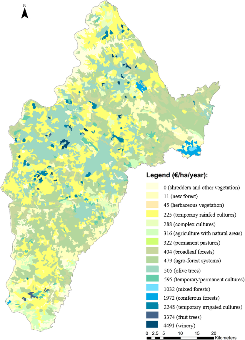
Fig. 2. Maximum opportunity costs of agro-environmental measures (AEMs) and silvo-environmental measures (SEMs) in the case study area across land-use types.
After the economic valuation of the different land uses, the PUs are created in step 4. The PUs are the portions of land that will be compared to one another in the MARZONE spatial prioritization model. The size of each PU is 200 × 200 m, which is equivalent to 4 ha. Once the spatial resolution is set, the eligible areas for the different zones are identified, followed by the relevant cost estimation within each 4 ha PU. Pixels without suitable areas for the implementation of the SEMs and AEMs, such as urban or industrial areas, are excluded from further analysis. Excluding these unsuitable areas, 70 327 PUs remain in total.
The next step 5 involves the identification of the conservation features in the >70 000 PUs. The selected conservation features consist of two different habitat types (low-density Montado and high-density Montado) and 22 different species (mainly birds), the occurrences of which are analysed for each PU. These 22 species were identified as playing a key role in the open low-density and high-density Montado ecosystems, and hence are important conservation features. Most of the birds’ spatial occurrence was based on the Instituto da Conservação da Natureza e da Biodiversidade (ICNB) bird atlas with a 10 × 10 km spatial resolution (ICNB 2008), while for the remaining bird data were obtained through LIFE projects (Silva & Pinto Reference Silva and Pinto2006, CEAI 2011). Data for fauna features had the same spatial resolution (Cabral et al. Reference Cabral, Queiroz, Trigo, Bettencourt, Ceia, Faria and Farrobo2008). For species whose presence was represented by points, a buffer of 5 km around those points was estimated to represent species distribution (e.g., Bonelli’s eagle; CEAI 2011). All biodiversity and habitat feature data were initially rastered for the eligible areas at a 25 × 25 m resolution and later aggregated to a 200 × 200 m resolution to match the PU resolution using ArcGIS v.10.4.1. In a series of meetings with experts of the ICNF, the potential of the conservation measures to protect each species was evaluated (Table 2). A total of 40% of the species are solely addressed by the two AEMs and a third solely by one or both SEMs. The remainder are conserved under both types of measures.
Table 2. Conservation features (species) targeted by the different measures.

AEM = agro-environmental measure; SEM = silvo-environmental measure; IUCN = International Union for Conservation of Nature; NA = not applicable.
Following step 5 is the establishment of the conservation targets for the habitats and species in step 6. The conservation targets for both the Montado habitats and 22 different species are defined at preservation levels of 10%, 20% and 30% of current levels following existing ICNF objectives.
All spatial data were initially converted into a raster format with a spatial resolution of 25 × 25 m and subsequently aggregated to the level of a PU of 200 × 200 m. This includes the species abundance in the case study area and the estimated opportunity costs of alternative land uses should a PU be selected for conservation purposes. Once the files with spatial input data were prepared for MARZONE v.2.01 in step 7, step 8 involved the calibration of: (1) the FPF in order to weight the importance of meeting a conservation target in relation to its costs; and (2) the BLM in order to weight the importance of minimizing boundaries and to fix the costs of having boundaries between two zones selected by MARZONE (see Eq. (1)). The former is calibrated based on the MARZONE best practice guidelines (Watts et al. Reference Watts, Steinback and Klein2008b). Defining the boundary costs between zones is more arbitrary, as it depends on the desired degree of clustering of areas in the solutions. Here, we chose to run a series of different scenarios increasing zone boundary costs, and then to fix these costs at their midpoint.
After the calibration, the final step 9 was to run MARZONE in order to identify priority areas that meet the conservation targets whilst minimizing costs. In the spatial analysis presented here, each MARZONE run had 10 million iterations and the runs were repeated 100 times for each conservation target, producing 100 different solutions. Among these 100 runs, MARZONE identifies the run that scores best on the objective function and provides the PU’s selection frequency. The latter is interpreted as a proxy for their irreplaceability.
Results
Prioritization of conservation measures
Fig. 3(a–d) shows the results where each type of measure is most frequently prioritized under the three conservation targets. The higher the conservation target, the larger the area selected by MARZONE to preserve the habitats and species involved. The increase in area size follows a more or less proportionate pathway with the increase in conservation target, with 57 000 ha of land selected for AEMs and SEMs under the 10% conservation target, 128 000 ha under the 20% conservation target and 208 000 ha under the 30% target (Table 3). Under the latter conservation target, almost two-thirds of the land in the case study area (74%) is selected for nature protection purposes. Only 20% of all the land is needed for SEMs and AEMs to reach the lowest conservation target of 10%.

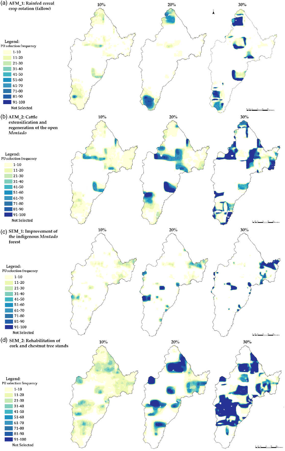
Fig. 3. Marxan with Zones (MARZONE) selected priority areas for agro-environmental measures based on their selection frequency, considering 10%, 20% and 30% conservation targets. (a) AEM_1: Rainfed cereal crop rotation (fallow); (b) AEM_2: Cattle extensification and regeneration of the open Montado; (c) SEM_1: Improvement of the indigenous Montado forest; (d) SEM_2: Rehabilitation of cork and chestnut tree stands. Planning units in dark blue had a high selection frequency in this region. Areas in light yellow had a very low selection frequency, while areas in white were not selected for conservation in the MARZONE runs.
Table 3. Selected planning units and associated economic and financial costs for agro-environmental measures (AEMs) and silvo-environmental measures (SEMs) across the case study area for different conservation targets.

NA = not applicable.
SEM_2 (rehabilitation of cork and chestnut tree stands) is the most frequently selected measure. Approximately 48% of the selected PUs apply this measure, followed by AEM_2 (livestock extensification and regeneration of open Montado), which is applied on c. 27% of the selected PUs. The rotation of rain-fed cereal crops (AEM_1) is selected in c. 14% of the selected PUs, while the improvement of native Montado forest is chosen least often (10% of the selected PUs propose this measure). The latter may not come as a surprise in view of the fact that the spatial distribution of remaining patches of dense Montado across the case study area is limited to the central-eastern part of the existing protected areas in the north and to the north-western part of the existing protected areas in the south (see Supplementary Fig. S1).
From Fig. 3 and Supplementary Fig. S3, it can be seen that SEM_1 is perhaps not unsurprisingly mostly chosen in existing protected areas (75%), whereas SEM_2 and the AEMs are found equally often outside of existing protected areas or along the edges of protected areas (AEM_1 is found for 63% in existing protected areas, AEM_2 for 52% and SEM_2 for 50%). Some patches of both SEMs and AEMs are located in the planned ecological corridor (SEM_2: 23%; AEM_2: 13%; AEM_1: 7%; SEM_1: 4%). Under the 30% conservation target, most of the AEM_2 is equally inside and outside of existing protected areas (54%), while most of the AEM_1 is concentrated in the protected area in the southern part of the study area and fragmented along the western border from the northern to the central part (Supplementary Fig. S3(c)). Although the ecological corridor seems to be primarily suited for SEM_2 under the 20% and 30% conservation targets, the AEMs gradually increase in this ecological zone when the conservation targets are increased from 10% to 30%.
Economic and financial costs
The economic opportunity costs of the selected PUs under the three conservation targets are presented in Table 3. These economic opportunity costs are not the same as the financial compensation levels that farmers get paid if they participate in the SEM and AEM programmes in the protected areas. The latter are much lower and fixed by the Portuguese Ministry of Agriculture. Although their calculation is in principle based on cost incurred and income foregone by the farmer for participating in the programme and the European Commission (2005) indicates that “in duly justified circumstances, an incentive payment of up to 20% may be paid,” they seem only loosely related to the economic opportunity costs of land in the study area (Santos et al. Reference Santos, Clemente, Brouwer, Antunes and Pinto2015). The total financial costs based on the selected PUs for the different measures are also presented in Table 3 and differ considerably from the total economic costs. The payment levels are based on information provided by the SEM and AEM programmes (see Table 1), where the exact payment per hectare depends on the size of the area that will be enrolled in the programme. The payments used in this study are the midpoint estimates of the payment ranges across the area sizes and varied between €33.0 ha−1 year−1 for AEM_2 to €51.0 ha−1 year−1 for SEM_2 and €61.5 ha−1 year−1 for SEM_1. Farmers receive €58.5 ha−1 year−1 if they apply a fallow rotation scheme for growing cereals (AEM_1). As a result, the average financial cost per ha per year is constant under all three conservation targets when dividing the total financial costs by the area size under each SEM or AEM. By contrast, the average economic costs per ha per year differ across the three conservation targets because the compositions of the measures across the PUs differ under each conservation target.
The total economic costs associated with reaching the 10%, 20% and 30% conservation targets range from €13.5 million for the lowest conservation target of 10% to €47.4 million for the highest conservation target of 30%. The associated financial costs are merely a fraction (c. 20%) of these estimated economic costs. The SEM_2 and AEM_2 measures are most expensive, accounting together for c. 73% of the total economic costs. The most frequently selected measure of SEM_2, with the highest level of area cover, also makes up the largest share of the total economic costs (c. 47%), followed by AEM_2 (c. 26%). AEM_1 and SEM_1 constitute the smallest share in the total economic costs measures (c. 14% and 13%, respectively). Remarkably, the ranking of measures in terms of their financial costs based on current compensation levels is different from the one based on economic costs. Due to its large area cover, SEM_2 is also financially the most expensive measure, but SEM_1 constitutes the smallest financial cost share, while the ranking of the two AEMs is reversed when based on their financial costs: AEM_1 is financially more expensive than AEM_2, while the reverse holds when looking at their economic costs.
Discussion
The integrated ecological and economic modelling approach presented here provides policy-makers and decision-makers with valuable insight into the cost-effectiveness of current and future spatial planning of conservation areas. However, the spatial data and information burden in order to be able to carry out this type of spatial modelling is high. Furthermore, the reliability of the spatial analysis depends crucially on the available spatial input data, including both the type of spatial data and information, such as the key features underlying biodiversity or habitats, and the economic values of alternative land uses and the spatial resolution of these data. The data and information necessary to inform spatial policy planning and decision-making are not always ready available. For example, in this case study, 6 years of census data were available for birds. Habitat data were less frequently monitored, namely in 2006 and 2010 only. The collection of data and information about the economic opportunity costs of alternative land uses was equally troublesome and crucially dependent on land-cover and land-use maps on the one hand and agricultural census data on the other hand in order to be able to calculate the economic margins of different agricultural land uses. Such spatially explicit economic data are not ready available at either the local or regional scale.
The input data used in the spatial analysis presented here mainly reflect a static snapshot of current habitat and species conditions. Ideally, longer time series data are needed to be able to assess trends and properly establish baseline levels for the relevant biodiversity features. Due to limited data and information over a longer period of time, the robustness of our results was tested by determining the selection frequency of each PU among the 100 runs (ranging from 0 to 100), indicating the importance of the PUs for achieving the conservation targets. The results proved to be robust. More attention will need to be paid in future applications to alternative ways of assessing the sensitivity of the results, such as by introducing uncertainty margins around both the biophysical features of conservation targets and the economic opportunity costs of alternative land uses.
Despite the significance of the obtained results for Montado ecosystem conservation, a number of uncertainties underpin the obtained MARZONE outputs. Firstly, the inclusion of other conservation features data, such as plant biodiversity, might increase the accuracy and reliability of the spatial results. Secondly, the inclusion of locally important ecosystem service maps related to the Montado ecosystems such as carbon sequestration could support policy-making and decision-making by further broadening the spatially detailed outputs. Finally, uncertainties related to the acceptance of these findings should also be considered. The effectiveness of these measures relies not only on farmers’ and landowners’ acceptance of the AEMs and SEMs and associated payment levels, but also on decision-makers agreeing to pay these amounts of money to ensure AEM and SEM implementation.
Conclusions
Given increasingly limited budgets for nature protection, policy-maker demand for information about how to spend these budgets most efficiently across larger geographical areas has grown exponentially over recent decades. Spatial targeting of biodiversity hotspots and ecosystem services provision and payment differentiation are generally recommended as key principles for the design of economically efficient nature protection payment schemes (Wunder et al. Reference Wunder, Brouwer, Engel, Ezzine-de-Blas, Muradian, Pacual and Pinto2018). In this study, we applied MARZONE in order to assess the extent to which existing protected areas in the Montado agroforestry landscape in southern Portugal overlap with the selection of land based on different conservation targets for key habitat and biodiversity features. The important role of human activities in shaping the Montado landscape and the multifunctionality of the Montado ecosystem is reflected in the nature of most of the proposed measures. At the same time, we compared the estimated economic opportunity costs with the standard payment levels landowners and farmers receive for implementing SEMs and AEMs, which differ across area size but not across alternative land uses and hence income forgone for farmers participating in the nature conservation programmes. In conclusion, MARZONE not only identifies which types of AEMs are – economically speaking – preferred in terms of their cost-effectiveness, and hence answers the question of what measures to implement, but also informs policy-makers and decision-makers about the location of these measures, and hence answers the question of where to implement these measures in confined geographical areas.
More specifically, we find considerable overlap between the selected lands for SEMs that aim to protect the native Montado forest and to rehabilitate the cork and chestnut tree stands and currently protected areas, while the priority land for the two AEMs are found equally often inside and outside of existing protected areas or along the edges of protected areas.
The economic costs of reaching habitat and species conservation targets of 10%, 20% and 30% are substantial, and many orders of magnitude higher than the financial compensation levels paid to landowners and farmers, explaining the very limited uptake of the SEMs and AEMs in the case study area (Santos et al. Reference Santos, Clemente, Brouwer, Antunes and Pinto2015). In particular, the rehabilitation of cork and chestnut tree stands is a cost-effective solution in the case study area and should be prioritized, followed at a distance by livestock extensification and the regeneration of the open Montado. Land suitable for prioritizing the improvement of the native Montado forest is found most frequently inside protected areas, but is the least cost-effective according to our spatial analysis. Priority should be given to the AEMs instead. Here, we see that the average economic cost per hectare of prioritized land decreases significantly for cattle extensification and the regeneration of low tree density Montado as conservation targets increase from 10% (€257.3 ha−1 year−1) to 20% (€251.3 ha−1 year−1) to 30% (€200.6 ha−1 year−1) compared to dryland cereal crop rotation (€207.8, €169.5 and €196.2 ha−1 year−1, respectively).
Supplementary Material
To view supplementary material for this article, please visit https://doi.org/10.1017/S0376892919000249
Acknowledgements
The authors are especially grateful to Ana Cristina Cardoso (ICNF) for her help with the conservation features and Sérgio Godinho (University of Evora) for sharing his data on the distribution of the Montado ecosystem in the case study area.
Financial Support
The research presented in this paper was carried out with the financial support of the EU-FP7 project POLICYMIX: assessing the role of economic instruments in POLICY MIXes for biodiversity conservation and ecosystem services provision (grant agreement number 244065). Rute Pinto gratefully acknowledges the financial support obtained from the Portuguese national funding agency for science, research and technology (FCT) (postdoctoral grant number SFRH/BPD/90675/2012). The Center for Environmental and Sustainability Research (CENSE) is financed through the FCT-grant Strategic Project UID/AMB/04085/2013. R. Pinto and R. Brouwer also gratefully acknowledge the support of Agricultural Water Futures (AWF) and the Integrated Modelling Program for Canada (IMPC), funded under the Canada First Research Excellence Fund project Global Water Futures.
Conflict of Interest
None.
Ethical Standards
None.