


INTRODUCTION
Landscape modification by humans through agricultural expansion, expansion of human settlements and urbanization (Godefroid & Koedam Reference Godefroid and Koedam2003; Kerr & Deguise Reference Kerr and Deguise2004; Luck et al. Reference Luck, Ricketts, Daily and Imhoff2004) is the most important modern cause of habitat loss and habitat fragmentation (Saunders et al. Reference Saunders, Hobbs and Margules1991; Rozzi et al. Reference Rozzi, Primack, Feinsinger, Dirzo, Massardo, Primack, Ruiz, Feinsinger, Dirzo and Massardo2001; Fisher & Lindenmayer Reference Fisher and Lindenmayer2007). In particular, habitat fragmentation is the process whereby a continuous habitat is reduced in area and divided into several remnants (Primack Reference Primack1993) that can impose devastating and irreversible consequences on the regional biodiversity (Liu et al. Reference Liu, Dong, Deng, Liu, Zhao and Dong2014). Through this process, when native ecosystems become fragmented by changes in land use, these undergo noticeable changes in structure and composition, frequently leading to habitat loss or destruction.
Landscape ecology studies have demonstrated a relationship between biological conditions within patches (e.g. species richness and diversity) and small-scale environmental factors, such as the habitat heterogeneity derived from changes in vegetation structure (i.e. presence of herbs, shrubs and trees) caused by anthropogenic disturbances (López-Barrera et al. Reference López-Barrera, Armesto, Williams-Linera, Smith-Ramírez, Manson and Newton2007). However, at the landscape level, there is also an effect of the spatial attributes of patches (size, shape, slope, orientation and connectivity) on the biological conditions of the habitat (Saunders et al. Reference Saunders, Hobbs and Margules1991; Stenhouse Reference Stenhouse2004) that can influence many natural phenomena and ecological processes (Fu et al. Reference Fu, Liu, Ma and Zhu2004).
Several studies have looked at patch size as a predictor of species richness due to the increased habitat heterogeneity in larger patches. Thus, structurally more complex and heterogeneous habitats would provide more resources for the establishment of a larger number of species (the habitat heterogeneity hypothesis) (Pincheira-Ulbrich et al. Reference Pincheira-Ulbrich, Rau and Peña-Cortés2009). In particular, as the patch size decreases, patches become increasingly exposed to environmental conditions prevailing in the surrounding matrix. This produces an edge that involves the emergence of new properties and dynamics that, over time, can lead to an increasing deterioration of habitat quality at the edge compared to inner patch areas, thus affecting the survival of species within patches (Tilman et al. Reference Tilman, May, Lehman and Nowak1994; Santos & Tellería Reference Santos and Tellería2006).
Edges can be thought of as buffer zones across which environmental conditions change progressively with distance, leading to a significant impact on forest structure and dynamics (Ries et al. Reference Ries, Fletcher, Battin and Sisk2004). This process segregates the habitat into two ecotones: an edge (low-quality) habitat and an interior (high-quality) habitat (Murcia Reference Murcia1995; Ries et al. Reference Ries, Fletcher, Battin and Sisk2004; Fletcher Reference Fletcher2005). Edges can be either abrupt or gradual according to the variation in environmental features (Sánchez et al. Reference Sánchez, Vega, Peters and Monroy-Vilchis2003) and the degree of contrast between the matrix and the fragmented habitat. For example, agricultural matrices drastically alter the microclimatic conditions of forest patches by promoting moisture loss and increasing light intensity, insolation, temperature, evaporation and wind exposure along the interior–edge gradient (Saunders et al. Reference Saunders, Hobbs and Margules1991).
Several studies have documented that the edge effect fosters changes in the structure and composition of vegetation as a result of the different responses of species (Murcia Reference Murcia1995; Godefroid & Koedam Reference Godefroid and Koedam2003; Cayuela Reference Cayuela2006). Species may increase, decrease or show no changes in abundance according to the characteristics of the environmental gradient (Murcia Reference Murcia1995), as well as in response to changes in interspecific interactions. Such conditions facilitate the establishment of plant species typical of early successional stages, weeds associated with disturbance (Goosem Reference Goosem2007) and exotic species, thus leading to the progressive loss of native species (Cadenasso & Pickett Reference Cadenasso and Pickett2000; Fahrig Reference Fahrig2003; Ries & Sisk Reference Ries and Sisk2010).
Species loss usually follows a species assemblage pattern (Patterson & Atmar Reference Patterson and Atmar1986; Lindenmayer et al. Reference Lindenmayer, Fischer and Cunningham2005; Ries & Sisk Reference Ries and Sisk2010); that is, the sum of the differential responses of each species to the edge effect (Santos & Tellería Reference Santos and Tellería2006). So, both factors can be merged into only one factor, such as edge vulnerability. Such vulnerability depends on the environmental requirements of each species and, therefore, species density and importance value are suitable indicators of the species assemblages pattern, with the less abundant species being lost earlier than the most abundant, according to the sampling hypothesis (Bolger et al. Reference Bolger, Alberts and Soule1991). To identify the pattern of species assemblage loss caused by the edge effect, it is necessary to first identify functional response plant groups (Lavorela et al. Reference Lavorela, McIntyreb, Landsbergc and Forbesd1997). A functional response assemblage is a set of species that respond similarly to particular environmental conditions (Westoby & Leishman Reference Westoby, Leishman, Smith, Shugart and Woodward1997; Lavorel & Garnier Reference Lavorel and Garnier2002; Casanoves et al. Reference Casanoves, Pla and Di Rienzo2011). Examples of functional response groups are assemblages of species found commonly or solely in forest gaps or under a closed canopy, frost- or drought-resistant species and grazing-tolerant or -intolerant species, among others (Wilson Reference Wilson1999; Hooper et al. Reference Hooper, Solan, Symstad, Díaz, Gessner, Loreau, Naeem and Inchausti2002). For example, Woodward (Reference Woodward, Ernst-Detlef and Mooney1993) defines functional groups based on a set of microclimatic variables (climate response functional groups; Gomez-Mendoza et al. Reference Gomez-Mendoza, Galicia and Aguilar-Santelises2008).
As Mexico's pine-oak forests are subject to strong anthropogenic disturbances and since previous findings suggest these forests exhibit edge effects on the distribution of plants (López-Barrera et al. Reference López-Barrera, Armesto, Williams-Linera, Smith-Ramírez, Manson and Newton2007; Granados et al. Reference Granados, Serrano and García-Romero2014), it is necessary to determine how degraded forest fragments are at the edges and how patch size influences the edge effect in these fragments (Williams Reference Williams2003). The present study site is a fragmented forest area where the fragment size varies considerably. The aim of this study was to examine the influence of patch size on the presence of functional groups along an edge–interior gradient in a pine-oak forest. To this end, we characterized the changes in forest structure and composition in relation to patch size, identified species groups associated with the edge–interior gradient in patches of different sizes, computed vulnerability indices for the species in relation to the distance from the edge and correlated the functional groups identified with environmental factors likely determining their distribution and composition. Identifying the threshold distances from the edge effect is particularly important in order to prevent, to the extent possible, local extinctions of species and their potential consequences for the remaining forest habitat.
METHOD
Study area
The study was conducted in a peri-urban forest in the Sierra de Monte Alto mountain range (2400–3800 m above sea level), located 12 km northwest of Mexico City (see map in Appendix S1; available online). The climate in this mountain range is characterized by a mean annual temperature ranging between 12 and 18°C and a mean annual precipitation of 1000–1200 mm. These conditions favour the presence of mixed pine-oak forests (Pinus teocote and P. pseudostrobus with Quercus crassipes, Q. laurina, Q. rugosa, Q. lanceolata and Alnus firmifolia) in mid-altitude slopes of the sierra (Granados et al. Reference Granados, Serrano and García-Romero2014).
This zone has been affected by a range of environmental and social issues associated with land-use changes that fostered extensive deforestation in the early 1970s (Galicia et al. Reference Galicia, García-Romero, Gómez-Mendoza and Ramirez2007). However, a preliminary inspection showed that, despite its proximity to Mexico City, forest fragments in the area have remained untouched for the past 40 years; this was the reason for choosing this area to study the edge effect on vegetation. A 692-km2 quadrat encompassing all the remaining pine-oak forest patches in the area was selected; using geographic information system (GIS) software, all (83.3 km2) forest patches with a minimum area of 1 ha were mapped by means of a supervised classification of a 2011 image from Google Earth™ Planet Image Service. Patches were classified according to basic descriptive statistics: (a) size, (b) shape index, and (c) connectivity (Farina Reference Farina2007).
Field sampling
Twenty-nine pine-oak forest patches were sampled along 2-m wide edge–interior transects of variable lengths (50–250 m) depending on patch size (Montenegro & Vargas Reference Montenegro and Vargas2008). Each transect was divided into 10-m long sectors and patches were classified into small (1–10 sectors from the edge to the centre of the patch), medium (11–20 sectors) and large (21–25 sectors) size. The density, coverage and basal area of each tree and shrub species (Matteucci & Colma Reference Matteucci and Colma1982) were recorded for each sector, in addition to environmental factors including temperature (digital thermometer), humidity, soil moisture, quality of light through the open canopy and the global site factor (calculated from hemispherical photographs), slope angle and soil compaction (DICKEY-john® penetrometer) (Romero-Torres & Varela-Ramírez Reference Romero-Torres and Varela-Ramírez2011). In addition, the thickness of the litter layer and the percentage coverage of vegetation, litter and bare soil were also recorded.
Data analyses
Identification of patch classes and groups of species
To identify groups of species that respond to the edge effect in relation to patch size, a two-way indicator species analysis (TWINSPAN) (Hill Reference Hill1994) was applied to the species importance values matrix (LaPaix & Freedman Reference LaPaix and Freedman2010) using the software PC-ORD v.5.10. The species importance value was calculated using the formula:
 $$\begin{equation*}
{\rm{I}}{{\rm{V}}_{\rm{i}}}\;{\rm{ = }}\;{\rm{D}}{{\rm{R}}_{\rm{i}}}\;{\rm{ + }}\;{\rm{F}}{{\rm{R}}_{\rm{i}}}\;{\rm{ + }}\;{\rm{C}}{{\rm{R}}_{\rm{i}}}
\end{equation*}$$
$$\begin{equation*}
{\rm{I}}{{\rm{V}}_{\rm{i}}}\;{\rm{ = }}\;{\rm{D}}{{\rm{R}}_{\rm{i}}}\;{\rm{ + }}\;{\rm{F}}{{\rm{R}}_{\rm{i}}}\;{\rm{ + }}\;{\rm{C}}{{\rm{R}}_{\rm{i}}}
\end{equation*}$$
where DRi, FRi and CRi are, respectively, the relative density, relative frequency and relative coverage of the ith tree or shrub species.
Those species having similar importance values across all transect sectors (Eupatorium glabratum, Quercus obtusata, Solanum spp, Symphoricarpos microphyllus, Buddleja cordata, Arbutus xalapensis, Quercus crassifolia, Q. crassipes and Pinus teocote), as well as those species that were recorded in only one or two sectors (Agave salmiana, Alnus acuminata, Bouvardia ternifolia, Cestrum nitidum, Crataegus mexicana, Cupressus lindleyi, Garrya laurifolia and Opuntia ficus-indica) were excluded from this analysis.
The main groups of species derived from the TWINSPAN classification analysis were interpreted as the effect of an environmental gradient caused by the edge effect. Only those groups that represent abrupt changes in the composition were taken into account.
Differences in structure and composition in relation to patch size
Overall vegetation attributes (species richness, diversity and importance value) were tabulated according to patch size class. Diversity was expressed in terms of the Shannon–Wiener index, as calculated by the software Past (ver. 3). Differences in species composition between patch size classes were evaluated with the Jaccard and Morisita indices.
Plant species groups related to the edge effect
A detrended correspondence analysis (DCA) was conducted using the software PC-ORD v.5.10 (Hill Reference Hill1994) to explore whether the species composition of different patch size classes can be related to the presence of environmental gradients and to determine whether the species groups identified by TWINSPAN were consistent.
Vulnerability of species to the edge effect
Vulnerability refers to the intrinsic characteristic of a species to be adversely affected by environmental factors, which was not analysed directly in this case. Rather, we analysed vulnerability in an indirect way, through recognizing the optimal coverage and width of the species distribution by sector, assuming that low or nil values were indicative of vulnerability. The weighted averages method (Arzac et al. Reference Arzac, Chacón-Moreno, Llambí and Dulhoste2011) was used to calculate a species vulnerability index. The particular sector along the edge–interior gradient where each species reached its optimum coverage (Oik) was identified using the following equation:
 $$\begin{equation*}
{O_{ik}} = \ \frac{{\mathop \sum \nolimits_{j = 1}^n A{f_{ij\ }}{V_{kj}}}}{{\mathop \sum \nolimits_{j = 1}^n A{f_{ij}}}}
\end{equation*}$$
$$\begin{equation*}
{O_{ik}} = \ \frac{{\mathop \sum \nolimits_{j = 1}^n A{f_{ij\ }}{V_{kj}}}}{{\mathop \sum \nolimits_{j = 1}^n A{f_{ij}}}}
\end{equation*}$$
where Afij is the importance value of the i species in the j sector, Vkj is the value of the k environmental variable (distance, in this case) in the j sector and n is the total number of sectors. The width (Aik) of the distribution of each species per sector was estimated using the weighted standard distribution:
 $$\begin{equation*}
{A_{ik}} = \ \sqrt {\frac{{\mathop \sum \nolimits_{j = 1}^n A{f_{ij}}\left( {{V_{kj}} - {O_{ik}}} \right)}}{{\mathop \sum \nolimits_{j = 1}^n A{f_{ij}}}}}
\end{equation*}$$
$$\begin{equation*}
{A_{ik}} = \ \sqrt {\frac{{\mathop \sum \nolimits_{j = 1}^n A{f_{ij}}\left( {{V_{kj}} - {O_{ik}}} \right)}}{{\mathop \sum \nolimits_{j = 1}^n A{f_{ij}}}}}
\end{equation*}$$
In this case, the amplitude of Aik indicates the average interval of the presence of the species along sectors, which represents the interior–edge environmental gradient. These results are derived from the environmental requirements and the tolerance threshold of each species, so these findings make it possible to determine the level of vulnerability of some species to the presence of the edge effect. The vulnerability index values were plotted to show the location of the optimum coverage and the distribution width of each species along the edge–interior sectors; actual values were not used.
Relationship between the functional groups responding to the environmental gradient and patch size
A canonical correspondence analysis (CCA) was performed using the software PC-ORD v.5.10 (McCune & Mefford Reference McCune and Mefford2006) to identify functional groups that respond to environmental factors such as temperature, humidity, soil moisture, quality of light through of the open canopy and the global site factor, slope angle and soil compaction. In addition, the thickness of the litter layer and the percentage coverage of vegetation, litter and bare soil were also included. Monte Carlo permutations were performed to determine the statistical significance (p < 0.05) of the resulting eigenvalues.
RESULTS
Identification of patch classes and groups of species
Once patches were classified according to size, the TWINSPAN analysis (Fig. 1) arranged these patch size classes according to species composition into five large (4.2–6.6 km2) patches (1, 4, 7, 8 and 9), seven medium-sized (1.5–3.7 km2) patches (11, 14, 15, 16, 18, 20 and 24), and 17 small (<1.1 km2) patches (2, 3, 5, 6, 10, 12, 13, 17, 19, 21, 22, 23, 25, 26, 27, 28 and 29).

Figure 1 Two-way indicator species analysis of the 29 forest patches in relation to the species importance values (see Appendix S2 for species abbreviations). L = large patch; M = medium patch; S = small patch.
Differences in structure and composition in relation to patch size
Structure and composition were similar between large, medium and small patches (Table 1). The Jaccard index showed a slight similarity between large, medium and small patches; small patches were the most dissimilar with respect to medium (57%) and large (54%) patches (Table 2). The Morisita index values show that small and medium patches shared almost 84% of their species, whereas large patches displayed the greatest dissimilarity versus small (59%) and medium (58%) patches (Table 2).
Table 1 Composition of different patch size classes.

Table 2 Values for Jaccard and Morisita similarity indices between patch size classes.

Some species were restricted to certain patch size classes. The species not found in large patches were Abies religiosa, Bouvardia ternifolia, Buddleja parviflora, Cestrum nitidum, C. thyrsoideus, Fuchsia thymifolia, Opuntia ficus-indica, Pinus teocote, P. patula, Solanum cervantesii and Symphoricarpos microphyllus. The species absent from medium-sized patches were Agave salmiana, Bouvardia ternifolia, Buddleja cordata, B. parviflora, Cestrum thyrsoideus, Eupatorium spp, Fraxinus uhdei, Fuchsia thymifolia, Monnina ciliolata, Pinus leiophylla and P. teocote, while those not found in small patches were Agave religiosa, Buddleja cordata, Cestrum nitidum, Crataegus mexicana, Fraxinus uhdei, Garrya laurifolia, Gaultheria acuminata, Monnina ciliolata, Quercus laeta, Senecio sinuatus and S. microphyllus.
Plant species groups related to the edge effect
TWINSPAN (Fig. 2) revealed six different groups of plant species (two for each patch size) that were characteristic of edge and interior habitats. These groups were named 1L/E (Large/Edge), 2L/I (Large/Interior), 3M/E (Medium/Edge), 4M/I (Medium/Interior), 5S/E (Small/Edge) and 6S/I (Small/Interior). The DCA revealed that the species groups identified in TWINSPAN were maintained in the ordination, thus denoting the relationship between patch size, environmental gradient and species composition of plant groups within patches.
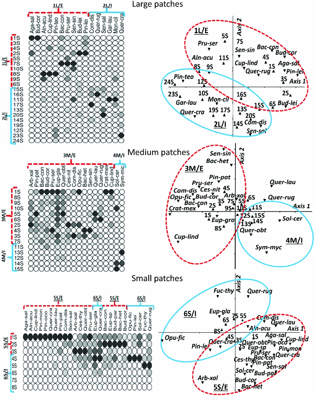
Figure 2 The results of the two-way indicator species analysis (left) and detrended correspondence analysis (right). The solid lines indicate the group of interior species and the broken lines indicate the group of species on the edge of the fragment in each case (see Appendix S2 for species abbreviations). 1L/E = edge functional group; 2L/I = interior functional group; 3M/E = edge functional group; 4M/I = interior functional group; 5S/E = edge functional group; 6S/I = interior functional group.
For large patches, group 1L/E included ten species found usually in the first ten sectors of a transect (i.e. between 0 and 100 m from the patch edge) and thus typical of the edge habitat. On the other hand, group 2L/I included six species usually found in sectors 11–25 (i.e. between 100 and 250 m from the patch edge) and thus typical of the interior habitat.
In medium-sized patches, two species groups also emerged: the 16 species included in group 3M/E were characteristic of edge habitats and were commonly found in the first ten sectors (0–100 m from the patch edge). Group 4M/I only included two species characteristic of the interior habitat and was usually found in sectors 10–15 (100–150 m from the patch edge).
In small patches, two species groups were distinguished: group 5S/E included 19 species characteristic of the edge habitat and commonly found in the first three sectors (0–30 m from the patch edge) and group 6S/I comprised seven species characteristic of the interior and commonly found in sectors 4–8 (40–80 m from the patch edge).
Vulnerability of species to the edge effect
Vulnerability indices for the species varied along the edge–interior gradient (see Appendix S3). For large patches, six of the ten edge species (Buddleia cordata, Agave salmiana, Pinus leiophylla, Baccharis conferta, Cupressus lindleyi and Alnus acuminata) had optimum coverage values, thus confirming their preference for edge areas. On the other hand, Prunus serotina, Senecio sinuatus, Buddleia cordata and Pinus teocote had wider distributions, some even reaching the patch interior (such as Buddleia cordata and Pinus teocote). However, as their optimum coverage occurred near the edge, these are also considered typical of edge sectors. Moreover, six species (Monnina ciliolata, Garrya laurifolia, Senecio salignus, Comarostaphylis discolor, Quercus rugosa and Q. crassipes) showed optimum coverage that confirmed their preference for interior habitats.
In medium-sized patches, Crataegus mexicana, Opuntia ficus-indica, Comarostaphylis discolor, Baccharis heterophylla, Quercus laurina and Senecio sinuatus had a narrow distribution restricted to the patch edge. On the other hand, Baccharis conferta, Buddleia cordata, Cupressus lindleyi, Arbutus xalapensis, Prunus serotina and Pinus patula were also characteristic of patch edges, but showed wider distributions. The species Eupatorium glabratum and Quercus obtusata showed a very wide distribution encompassing the entire edge–interior gradient, but the location of their optimum coverage suggests that edge conditions better fulfilled the environmental requirements of these species. For only two species (Solanum cervantesii and Symphoricarpos microphylla) did the location of their optimum coverage confirm their preference for interior habitats.
In small patches, Agave salmiana, Senecio salignus, Pinus teocote, Pinus montezumae, Cupressus lindleyi and Alnus acuminata showed a very narrow distribution, restricted entirely to the first sector. On the other hand, Quercus crassifolia, Q. laurina, Q. obtusata, Pinus patula, Cestrum thyrsoideum, Buddleja parviflora, B. cordata, Baccharis heterophylla, B. conferta, Comarostaphylis discolor, Prunus serotina, Eupatorium spp and Arbutus xalapensis showed a wider distribution, although their optimum coverage was located near the patch edge (sectors 1–3). Finally, the species Solanum cervantesii, Pinus leiophylla, Opuntia ficus-indica, Quercus crassipes, Q. rugosa, Eupatorium glabratum and Fuchsia thymifolia were also widespread species, but their optimum coverage was located towards the patch interior.
Functional groups in response to the environmental gradient and patch size
The CCA ordination showed sectors, species and environmental variables varying among patch sizes (Fig. 3). The eigenvalues (E) of the first three axes were as follows: for large patches, E axis 1 = 0.76, E axis 2 = 0.52, E axis 3 = 0.44; cumulative variance = 40%; for medium patches, E axis 1 = 0.82, E axis 2 = 0.43, E Axis 3 = 0.21; cumulative variance = 64%; and for small patches, E axis 1 = 0.67, E axis 2 = 0.49, E axis 3 = 0.27; cumulative variance = 77%. For each patch size, the ordination provided a significant representation of the species distribution and the environmental variables recorded (Monte Carlo permutation test, p < 0.05).

Figure 3 Canonical correspondence analysis diagrams of sectors, species and environmental variables for large, medium and small patches. The solid lines indicate the group of interior species and the broken lines indicate the group of species on the edge of the fragment in each case (see Appendix S2 for species abbreviations). EnvHum = humidity; SoilHum = soil moisture; EnvTemp = air temperature; SoilTemp = soil temperature; Opencan = open canopy; GSF = global site factor; Litterde = litter depth; %Litter = percentage of litter cover; %VegCove = percentage of plant cover; %BareSoil = percentage of bare soil; 1L/E = edge functional group; 2L/I = interior functional group; 3M/E = edge functional group; 4M/I = interior functional group; 5S/E = edge functional group; 6S/I = interior functional group.
For large patches, the functional group 1L/E was related to canopy openings, the global site factor, soil temperature and percentage plant cover (Fig. 3). Functional group 2L/I was related to slope and litter depth and cover. For medium patches, functional group 3M/E was related to humidity, soil moisture, air temperature, the global site factor, percentage plant cover, slope and litter cover (Fig. 3). On the other hand, functional group 4M/I was related primarily to litter depth and soil temperature. For small patches, functional group 5S/E was related to humidity, soil moisture and canopy opening. Functional group 6S/I was related primarily to air temperature, the global site factor and slope (Fig. 3).
DISCUSSION
The edge effect on the composition and structure of vegetation was influenced by patch size. Despite the high within-patch biotic heterogeneity, the exclusion of rare and cosmopolitan species revealed that patches share species according to size, thus indicating that similar ecological conditions prevail in patches of similar size (Saunders et al. Reference Saunders, Hobbs and Margules1991; Stenhouse Reference Stenhouse2004).
Plant species richness, diversity and evenness were very similar in the three patch size classes. This result does not agree with the findings of other similar studies that concluded that patch size can be a good predictor of species richness (Saunders et al. Reference Saunders, Hobbs and Margules1991; Tilman et al. Reference Tilman, May, Lehman and Nowak1994; Santos & Tellería Reference Santos and Tellería2006; Pincheira-Ulbrich et al. Reference Pincheira-Ulbrich, Rau and Peña-Cortés2009). However, according to the metapopulation theory, smaller areas may have a greater diversity due to increased heterogeneity and colonization rates (Ceccon Reference Ceccon2013). For instance, Saunders et al. (Reference Saunders, Hobbs and Margules1991) pointed out that a collection of small patches can encompass a wider range of habitats than a single large patch. By contrast, the β diversity analyses revealed substantial differences in species compositions between patches of different sizes, as there was only a 60% species similarity between patches as evaluated through the Jaccard and Morisita indices.
The fact that environmental gradients in fragments of different sizes result in different functional groups involves multiple underlying factors. Unlike medium and large patches, small patches have abrupt and narrow edges (30 m) that can be the result of multiple interferences from the external matrix. For example, they are more exposed to the entry of light and heat (Mitchell et al. Reference Mitchell, Bennett and Gonzalez2014), as well as to extreme and changing weather conditions (Asbjornsen et al. Reference Asbjornsen, Ashton, Vogt and Palacios2004). In addition, the structure of the habitat in small patches tends to be more simple, while connectivity is reduced, hence affecting not only the diversity of resources for the establishment of different species in interior areas (Pincheira-Ulbrich et al. Reference Pincheira-Ulbrich, Rau and Peña-Cortés2009), but also the dispersion of seeds coming from adjacent patches (Porensky & Young Reference Porensky and Young2016).
All of these changes lead to different properties and dynamics that, over time, affect the functional connectivity, sexual reproduction potential and survival of some species that are sensitive to patch edges (Tilman et al. Reference Tilman, May, Lehman and Nowak1994; Fahrig Reference Fahrig2003; Santos & Tellería Reference Santos and Tellería2006), hence reducing their population sizes and posing a greater risk of extinction (Fletcher Reference Fletcher2005).
On the other hand, the distribution of species in relation to the patch edge varied between patch sizes. The edge effect was noticeable in the first 100 m from the edge in large and medium patches (1L/E and 3M/E). By contrast, in small patches, there was a group of species (5S/E) that responded to the edge effect in only the first 30 m from the edge. Such different responses may be due to the level of contrast between the surrounding matrix and the fragmented habitat (Sánchez et al. Reference Sánchez, Vega, Peters and Monroy-Vilchis2003). For example, here we observed that smaller patches had a highly contrasting edge, causing a clear differentiation in species composition in the first sectors of the transect, which may be related to a high heterogeneity along the patch edge (Saunders et al. Reference Saunders, Hobbs and Margules1991; Ries et al. Reference Ries, Fletcher, Battin and Sisk2004).
These changes in species composition can be explained by the various types of response of species to edges (Murcia Reference Murcia1995; Cayuela Reference Cayuela2006). According to Ries et al. (Reference Ries, Fletcher, Battin and Sisk2004), a species may show a positive, negative or neutral response, depending on the type of edge found. We found that some species showed a neutral response to the edge (species with wide distributions along the edge–interior gradient), while the species that showed a positive or negative response to edges constituted the species groups with contrasting habitat preferences (edge versus interior).
Patch edges (1L/E, 3M/E and 5S/E) consistently showed higher species richness relative to interior habitats, consistent with the intermediate disturbance hypothesis, which states that the highest species diversity is achieved under medium-intensity disturbance; that is, when mortality agents act with moderate intensity, preventing the most competitive species from excluding the others (Sánchez et al. Reference Sánchez, Vega, Peters and Monroy-Vilchis2003). In this case, it would be important to examine the life strategies of species in the edge zone in order to determine whether native, secondary vegetation, weeds, exotic or invasive plant species predominate and to examine their role in community dynamics.
The vulnerability analysis identified the threshold response of some species to fragmentation. The vulnerability of species was generally low, as eight species in particular were not able to penetrate the edge habitat in large patches, two in medium patches and one in small patches. These species’ response thresholds are driven by environmental factors and are usually abrupt in agricultural matrices such as those prevailing in the study area (Saunders et al. Reference Saunders, Hobbs and Margules1991). These results are relevant for identifying species that can serve as indicators of edges or disturbances or, conversely, of well-preserved habitats (Lindenmayer et al. Reference Lindenmayer, Fischer and Cunningham2005; Goosem Reference Goosem2007; Ries & Sisk Reference Ries and Sisk2010). Identifying species that are particularly vulnerable to the edge effect provides a tool to prevent, to the extent possible, the likely disappearance of species in fragmented landscapes (Patterson & Atmar Reference Patterson and Atmar1986; Cadenasso & Pickett Reference Cadenasso and Pickett2000; Fahrig Reference Fahrig2003).
The CCA revealed that the environmental factors most closely related to the occurrence of functional response plant groups were humidity, soil moisture and light (canopy opening and the global site factor), which determined the presence of edge functional groups (1L/E, 3M/E and 5S/E) in patches of different sizes. These results are consistent with those of Saunders et al. (Reference Saunders, Hobbs and Margules1991), who characterized edges as having higher insolation and evaporation, leading to the loss of soil moisture and increased wind exposure, which in turn negatively affect native vegetation. Several studies have shown that the increase in heat radiation can be detected up to 100 m from the edge into a patch (Ceccon Reference Ceccon2013).
In this study, litter cover, depth, slope and soil and air temperature were the main factors associated with the presence of interior functional groups (2L/I, 4M/I and 6S/I), which is consistent with other studies that showed that wind and a greater exposure to the elements increase towards the edge; this prevents accumulation of litter on the patch edge (Geiger Reference Geiger1965), retains soil moisture and maintains the higher density and activity of soil microorganisms that are responsible for litter decomposition (Saunders et al. Reference Saunders, Hobbs and Margules1991).
Our study focused on the combined response of functional groups, but at the same time emphasized the unique individual response of each species to changes in landscape, habitat loss and edge effects (Lindenmayer & Franklin Reference Lindenmayer and Franklin2002). Detailed study of the response of a single species may not significantly elucidate the general pattern of change in larger plant groups, but identifying general patterns involving many species may be particularly useful for management and conservation.
CONCLUSION
We found that patches of different sizes had similar species richness and diversity, but differed in species composition and other characteristics. In small patches, the edge effect was detectable in the first 30 m along the edge–interior gradient, but in medium and large patches, this effect could be observed over the first 100 m. In all patch sizes, two distinct plant groups responding to the edge effect were found. The presence of species in these functional groups was associated with particular environmental factors: the edge functional assemblage was associated with gradients of soil and air moisture, as well as light (canopy opening and the global site factor), while the interior functional assemblage was associated mostly with litter depth and cover, slope and air and soil temperature.
These findings help to identify species that are useful as indicators of edge or disturbance effects, in addition to evaluating the vulnerability level of interior species within natural vegetation patches, which are generally used as indicators of habitat conservation. The fragmentation response thresholds of plant species provide useful tools for preventing the likely disappearance of species.
ACKNOWLEDGEMENTS
This study was part of the doctoral dissertation of C. Granados at the Postgraduate School of Geography, UNAM. María Elena Sánchez-Salazar contributed to the English translation of the manuscript.
FINANCIAL SUPPORT
This work was supported by the DGAPA-PAPIIT (grant number IN301414) and a post-doctoral scholarship awarded by the Coordination of Scientific Research, UNAM.
CONFLICT OF INTEREST
None.
ETHICAL STANDARDS
None.
Supplementary material
To view supplementary material for this article, please visit https://doi.org/10.1017/S0376892917000595


