1. Introduction
Environmental issues have uncertain outcomes that cannot be accurately predicted because our knowledge of the underlying mechanisms governing the environmental state is limited. For example, it is generally considered that reducing CO 2 emissions would decrease the average atmospheric and oceanic temperatures or that protecting a certain species would be unquestionably good. Such perspectives should encourage governments to adopt the environmental policies required in this regard. However, in fact, the effects of environmental policies cannot be easily foreseen. Reducing CO 2 emissions might increase such average temperatures, and protecting some species might endanger others, which could discourage a government from adopting the related environmental policies. In other words, when governments adopt environmental policies, they should consider the uncertainty regarding the policies' results. Otherwise, policy makers can neither analyze the rationality of an environmental policy correctly nor propose appropriate policies. Therefore, the notion of uncertainty should be incorporated into the analyses of environmental policy making. This paper aims to investigate the effects of ambiguity (or Knightian uncertainty) on natural capital investment within the framework of a simple two-period model by employing the framework of Kogan and Wang (Reference Kogan and Wang2002) and Miao (Reference Miao2004).Footnote 1 Note that in this paper, the definition of natural capital is based on that in Ekins (Reference Ekins, Ekins and Max-Neef1992) and Ekins et al. (Reference Ekins, Simon, Deutsch, Folke and De Groot2003) by which capital is assumed to serve four distinct types of environmental functions. These functions are providing resources for production, absorbing waste from production, providing life support, and preserving the beauty of the wilderness and other natural areas.
Economists recognize that the distinction between risk and ambiguity is significant from theoretical and practical viewpoints. In the literature, while risk captures the situation in which a probability measure about future events is uniquely assigned, ambiguity captures the situation in which randomness in the future is represented by a set of probability measures or a non-additive measure (or a capacity), owing to imprecise information.Footnote 2 Since Knight (Reference Knight1921) was the first to highlight the importance of the distinction between risk and ambiguity, ambiguity is also referred to as Knightian uncertainty.Footnote 3 Based on Knight's argument, Ellsberg (Reference Ellsberg1961) suggests the empirical importance of the distinction between risk and ambiguity.
Decision theory literature considers that a decision maker's information is insufficient to pin down a unique probability for the likelihood of unknown events and that his or her beliefs can be captured well by a set of probability measures and not by a unique probability measure.Footnote 4 For example, various researchers have predicted the effects of environmental policies on average atmospheric or oceanic temperatures over the next several decades and have discussed possible scenarios or distributions of these effects. However, we lack reliable criteria to pin down the true scenario or distribution of the effects of environmental policies. The notion of Knightian uncertainty enables us to analyze these scenarios. Imprecise information makes people cautious when making decisions. In order to analyze such behavior from a normative point of view, Gilboa and Schmeidler (Reference Gilboa and Schmeidler1989) show that decision makers' beliefs are captured by a set of probability measures and their preferences are represented by the minimum of their expected utility over their set of probability measures. Applications of MEU and CEU to finance (Dow and Werlang Reference Dow and Werlang1992; Epstein and Wang Reference Epstein and Wang1994) and job search (Nishimura and Ozaki Reference Nishimura and Ozaki2004) shed further light on the distinction between risk and ambiguity.
The importance of ambiguity is also recognized in the environmental economics literature. Some studies from the late 1990s and the early 2000s, for example Woodward and Bishop (Reference Woodward and Bishop1997) and Lange (Reference Lange2003), emphasize the importance of ambiguity from the viewpoint of environmental economics and derive several significant policy implications for environmental uncertainty. However, a theoretical issue remains unaddressed in their studies: they introduce uncertainty directly into stylized economic models without providing decision theoretic foundations. Recent developments in decision theory enable us to analyze optimal environmental policies based on more rigorous axiomatic foundations. Asano (Reference Asano2010) examines the precautionary principle from the viewpoint of ambiguity. Asano (Reference Asano2010) derives the optimal timing of environmental policies under ambiguity and shows that an increase in ambiguity prompts a government into adopting the optimal environmental policy. Brock and Xepapadeas (Reference Brock, Xepapadeas, Arnott, Greenwald, Kanbur and Nalebuff2003) consider an environmental system with global characteristics and analyze a situation in which a regulator is uncertainty averse and the regulatees are risk averse. Brock and Xepapadeas (Reference Brock, Xepapadeas, Arnott, Greenwald, Kanbur and Nalebuff2003) identify the public bad externality effect and precautionary effect. The latter effect is induced by heterogeneity (that is, a regulator is uncertainty averse and the regulatees are risk averse). Within the framework of Hansen and Sargent's (Hansen and Sargent (Reference Hansen and Sargent2001) analysis of model uncertainty,Footnote 5 Athanassoglou and Xepapadeas (Reference Athanassoglou and Xepapadeas2012) analyze optimal pollution control policy under ambiguity and show that, while an increase in model uncertainty always increases investment in damage-control technology, it does not always do so in optimal mitigation. Gonzalez (Reference Gonzalez2008) introduces robust control theory to Hoel and Karp's (Reference Hoel and Karp2001) model, in which the policy maker is assumed to choose pollution taxes to minimize the discounted expected sum of pollution damages and abatement costs. Gonzalez (Reference Gonzalez2008) considers a situation in which a policy maker cannot pin down the true model but has some set of possible alternative models when faced with environmental problems. Gonzalez (Reference Gonzalez2008) shows that an increase in either uncertainty about the model or risk about abatement costs increases expected steady-state pollution taxes, and the effect of introducing model uncertainty on expected steady-state pollution taxes and stock pollutants is relatively small for high levels of model uncertainty. Furthermore, Gonzalez (Reference Gonzalez2008) suggests that the precautionary principle to the problem posed by Hoel and Karp (Reference Hoel and Karp2001) is theoretically supported within the framework of model uncertainty. Moreover, Vardas and Xepapadeas (Reference Vardas and Xepapadeas2010) analyze biodiversity management rules under ambiguity and provide a measure of the impact of adopting precautionary approaches within a framework of ecosystem management. Millner et al. (Reference Millner, Dietz and Heal2013) incorporate Klibanoff et al.'s (Reference Klibanoff, Marinacci and Mukerji2005) model into environmental economics and show that, in some simple examples, an increase in ambiguity aversion increases the optimal abatement level within a static framework.Footnote 6 Based on Klibanoff et al. (Reference Klibanoff, Marinacci and Mukerji2005), Treich (Reference Treich2010) analyzes the effects of ambiguity aversion in a standard static value of a statistical life (VSL) model and shows that the existence of ambiguity over baseline mortality increases the VSL when a decision maker is ambiguity averse.
In this paper, we introduce Knightian uncertainty into a simple two-period model and derive the optimal amount of natural capital investment by a government. Then, we analyze how the degree of Knightian uncertainty affects such optimal investment. Moreover, we show that the degree of Knightian uncertainty affects the size of the government's natural capital investment and that the direction of the effect of Knightian uncertainty depends on the nature of the uncertainty: whether it is uncertainty about the future level of natural capital or about the return from savings. More precisely, we show that an increase in uncertainty about the return from savings increases the amount of government investment, while an increase in uncertainty about the effect of natural capital investment reduces the optimal investment.
In analyzing the effects of Knightian uncertainty, we restrict our attention to the case in which the degree of uncertainty is captured by normal distributions. However, this assumption might be restrictive. Moreover, in general, the externalities associated with environment capital are not included in the definition of gross domestic product (GDP). However, we assume that the government is able to internalize all externalities. It should be mentioned that because of these two simplifying assumptions, we are able to derive analytical solutions and perform comparative static analyses.
The rest of this paper is organized as follows. In section 2, after defining the concept of natural capital, we develop a model of natural capital investment under ambiguity and derive the main results. Section 3 concludes.
2. The model
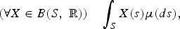
In this section, we develop a simple two-period model of natural capital investment. Assuming that the government is an MEU-maximizer (i.e., that its beliefs are captured by a set of probability measures and its preferences are represented by the minimum of its expected utility over that set), we derive the optimal amount of natural capital investment under Knightian uncertainty. Since we focus on the MEU framework, our model captures the situation in which the government is cautious about the effect of its natural capital investment owing to imprecise information. Before we provide a formal model, we define the notion of natural capital in the following subsection. Throughout this paper, we assume that there are two periods, the present (t = 1) and the future (t = 2). Let S be the space of the states of the world, let
 ${\cal F}$
be a σ -algebra of S, and let
${\cal F}$
be a σ -algebra of S, and let
 $\lpar S\comma \; {\cal F}\rpar $
be a measurable space. Let B(S, ℝ) denote the space of bounded functions from S into ℝ.
$\lpar S\comma \; {\cal F}\rpar $
be a measurable space. Let B(S, ℝ) denote the space of bounded functions from S into ℝ.
2.1. Natural capital
In this subsection, we provide the definition of the notion of natural capital (also called ecological capital or environmental capital) based on Ekins (Reference Ekins, Ekins and Max-Neef1992) and Ekins et al. (Reference Ekins, Simon, Deutsch, Folke and De Groot2003).Footnote 7 In the environmental economics literature, natural capital is divided into capital serving four distinct types of environmental functions. As stated in Ekins et al. (Reference Ekins, Simon, Deutsch, Folke and De Groot2003: 167), the first type is the provision of resources for production, that is, the raw materials that become food, fuel, metals and timber. The second is the absorption of waste from production, both from the production process and from the disposal of consumer goods. The third is providing life support to produce climate and ecosystem stability and shield all living beings from ultraviolet radiation by means of the ozone layer. The last type improves human welfare by preserving the beauty of the wilderness and other natural areas, which is also called amenity services. In line with the definition of natural capital presented above, we can elaborate a definition of positive and negative investments in natural capital. Positive investments, for example, could mean protecting endangered species, recycling, or fertilizing the soil. In contrast, negative investments could include the indiscriminate exploitation of forests or mines. The effects of these investments on the environment cannot be easily foreseen. For example, protecting some species might endanger other species. Thus, the manner in which ambiguity affects environmental policies established by governments needs to be examined. This is the main theme of this paper.
2.2. Ambiguity about future returns to natural capital
In this subsection, we provide a model of natural capital investment. In general, the effects of natural capital investment cannot be easily predicted. For example, reducing CO2 emissions might increase the average atmospheric or oceanic temperatures and result in accelerated global warming; protecting some species could endanger other species. That is, the effects of reducing CO2 emissions on global warming and the effects of offering protection to some species over other species are ambiguous. Although well-designed policies can generally eliminate the possibility of certain problems (e.g., that protection to certain species can be detrimental to other species), for some problems, it is not easy to develop well-designed policies. Vardas and Xepapadeas (Reference Vardas and Xepapadeas2010: 380) point out that
the development of management rules that could help to prevent loss of biodiversity is a desirable goal. The attainment of this goal is hindered, however, both by the complexity of ecosystems and by important and interrelated uncertainties, a number of which include sources such as major gaps in global and national monitoring systems; the lack of a complete inventory of species and their actual distributions; limited modelling capacity and lack of theories to anticipate thresholds; emergence of surprises and unexpected consequences.
Moreover, as pointed out by Mori et al. (Reference Mori, Katsukawa and Matsuda2001), the effect of protection, in particular, for overexploited species, is uncertain. Mori et al. (Reference Mori, Katsukawa and Matsuda2001) investigate the case of Southern bluefin tuna that were heavily depleted in the mid-1980s and for which the fishing quota has been restricted since 1985. Mori et al. (Reference Mori, Katsukawa and Matsuda2001) point out that the spawning stock biomass trend is highly vulnerable to age-composition dynamics.Footnote 8 Therefore, it is appropriate to assume that the effects of natural capital investment can be ambiguous and can be captured by a random variable. In the following, we analyze the cases in which (1) the effect of natural capital investment is uncertain and the return from saving is deterministic, and (2) the effect of natural capital investment is deterministic and the return from saving is uncertain. In this paper, we formulate our set-up in line with the literature on finance, which includes Arrow (Reference Arrow1965) and Miao (Reference Miao2004).
2.2.1. Linear cost function
First, we analyze the case in which the effect of natural capital investment is uncertain and the return from saving is deterministic. In addition, we assume that the government's cost function is linear. Let X(s) denote the effect of natural capital investment in state s at time t = 2, where X∈ B(S,ℝ). Let H 1 and H 2 be natural capital at t = 1 and t = 2, respectively, and let H 2:ℝ × ℝ → ℝ be defined by
 $$H_2 \lpar X\lpar s\rpar \comma \; M\rpar \equiv \lpar 1 - \delta\rpar H_1 + MX\lpar s\rpar \comma$$
where δ∈ [0,1] denotes the depreciation rate and M ∈ ℝ denotes the amount of natural capital investment. Equation (1) states that the natural capital at t = 2, H 2, is determined by the natural capital at t = 1, H 1; the amount of natural capital investment, M; and the effect of the investment, X(s). The positive depreciation rate, δ, suggests that if the government does not act to protect the environment, then the natural capital depreciates accordingly. Even if we assume that δ = 0, this does not affect the following analyses. It is noteworthy that the amount of natural capital investment, M, can take negative values. Negative investment in this context means that the government destroys the environment (natural capital) for the purpose of constructing roads or bridges. Let Y 1 and p denote the GDP at t = 1 and the price of natural capital investment, respectively. The amount of consumption at t = 2 is then c 2 = R(Y 1 − pM − c 1) + Y 2, where R denotes the return from saving; c 1 denotes the amount of consumption at t = 1; and Y 1 and Y 2 are the GDP at t = 1 and t = 2, respectively. According to the definition of natural capital presented in subsection 2.1, it is appropriate to assume that the GDP depends on the level of natural capital. Therefore, we assume that Y 1 and Y 2 depend on the amounts of natural capital H 1 and H 2, respectively. That is, Y 1 = Ψ (H 1) and Y 2 = Ψ (H 2). In general, the externalities associated with environmental capital are not included in the traditional definition of GDP. However, we assume that the notion of GDP includes the value of all environmental services and thus includes the positive external effects from natural capital. In this paper, for ease of analysis, the government is assumed to optimize the objective function by accounting for the external effects. Function Ψ :ℝ → ℝ is assumed to be concave and continuously differentiable with Ψ′(·) > 0 and Ψ″ (·) ≤ 0. We assume that utility function u:ℝ → ℝ is concave and twice-continuously differentiable, such that u′(·) > 0 and u″ < 0.
Next, in order to derive the optimal amount of natural capital investment, we specify the government's set of probability measures. Following Kogan and Wang (Reference Kogan and Wang2002) and Miao (Reference Miao2004), we consider the following set of probability measures:
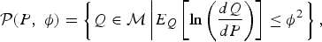 $${\cal P}\lpar P\comma \; \phi\rpar = \left\{Q \in {\cal M} \left\vert E_Q \left[\ln \left({dQ \over dP} \right)\right]\leq \phi^2 \right. \right\}\comma$$
where
 ${\cal M}$
denotes the set of all probability measures on
${\cal M}$
denotes the set of all probability measures on
 $\lpar S\comma \; {\cal F}\rpar $
, dQ/dP is the density of Q with respect to P, and P is the reference probability measure that can be interpreted as the true probability measure. The larger the value of ϕ, the larger the set
$\lpar S\comma \; {\cal F}\rpar $
, dQ/dP is the density of Q with respect to P, and P is the reference probability measure that can be interpreted as the true probability measure. The larger the value of ϕ, the larger the set
 ${\cal P}\lpar P\comma \; \phi \rpar $
, which suggests that beliefs about the effects of natural capital investment cannot be clearly identified owing to ambiguity increase.
${\cal P}\lpar P\comma \; \phi \rpar $
, which suggests that beliefs about the effects of natural capital investment cannot be clearly identified owing to ambiguity increase.
Let P be the reference probability measure corresponding to a normal distribution with mean μ
x
and variance σ
x
2. It is assumed that all of the government's beliefs on the effects of natural capital investment in
 ${\cal P}\lpar P\comma \; \phi\rpar $
have normal distributions. Furthermore, each probability measure in
${\cal P}\lpar P\comma \; \phi\rpar $
have normal distributions. Furthermore, each probability measure in
 ${\cal P}\lpar P\comma \; \phi\rpar $
has variance σ
x
2 and mean μ
x
− v for some v ∈ ℝ.Footnote
9
The presence of ambiguity does not enable the government to accurately identify the mean, μ. Note that mean μ
x
− v is not always less than μ
x
, since v can take a negative value. As Kogan and Wang (Reference Kogan and Wang2002) show, the set
${\cal P}\lpar P\comma \; \phi\rpar $
has variance σ
x
2 and mean μ
x
− v for some v ∈ ℝ.Footnote
9
The presence of ambiguity does not enable the government to accurately identify the mean, μ. Note that mean μ
x
− v is not always less than μ
x
, since v can take a negative value. As Kogan and Wang (Reference Kogan and Wang2002) show, the set
 ${\cal P}\lpar P\comma \; \phi\rpar $
is isomorphic to the following set:
${\cal P}\lpar P\comma \; \phi\rpar $
is isomorphic to the following set:
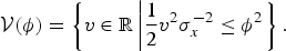 $${\cal V}\lpar \phi\rpar = \left\{v\in {\open R}\left\vert {1 \over 2}v^{2}\sigma _{x}^{-2}\leq \phi ^{2} \right. \right\}.$$
The larger the value of ϕ, the larger the set
 ${\cal V}\lpar \phi \rpar $
, which means that the set of government's beliefs,
${\cal V}\lpar \phi \rpar $
, which means that the set of government's beliefs,
 ${\cal P}\lpar P\comma \; \phi\rpar $
, becomes large as ϕ increases. Since we focus on the model within the MEU framework, as the set of the government's priors expands owing to increases in ϕ, the government becomes cautious about the effect of natural capital investment and does not invest in the environment. Therefore, parameter ϕ can be interpreted as the degree of ambiguity. As in standard analyses, we assume that risk is captured by variance σ
x
2. Thus, the notions of risk and ambiguity are differentiated by σ
x
2 and ϕ, respectively. If the degree of ambiguity is set to be zero, that is, if ϕ = 0, then the set of probability measures,
${\cal P}\lpar P\comma \; \phi\rpar $
, becomes large as ϕ increases. Since we focus on the model within the MEU framework, as the set of the government's priors expands owing to increases in ϕ, the government becomes cautious about the effect of natural capital investment and does not invest in the environment. Therefore, parameter ϕ can be interpreted as the degree of ambiguity. As in standard analyses, we assume that risk is captured by variance σ
x
2. Thus, the notions of risk and ambiguity are differentiated by σ
x
2 and ϕ, respectively. If the degree of ambiguity is set to be zero, that is, if ϕ = 0, then the set of probability measures,
 ${\cal P}\lpar P\comma \; \phi\rpar $
, turns out to be a singleton. In this case, the notion of ambiguity cannot be captured, and our model is reduced to the standard expected utility model.
${\cal P}\lpar P\comma \; \phi\rpar $
, turns out to be a singleton. In this case, the notion of ambiguity cannot be captured, and our model is reduced to the standard expected utility model.
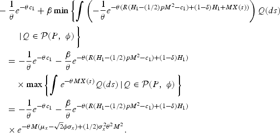
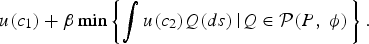
Now, we formulate a simple two-period natural capital investment model under Knightian uncertainty. The government is supposed to choose c 1 and M in order to maximize the following objective function:
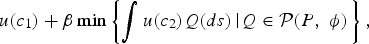 $$u\lpar c_{1}\rpar + \beta \min \left\{\vint u\lpar c_{2}\rpar Q\lpar ds\rpar \left\vert Q\in {\cal P}\lpar P\comma \; \phi \rpar \right. \right\}\comma$$
where c 2 = Ψ (H 1) − pM − c 1 + Ψ (H 2). We assume here that the objective is a function of only private consumption as in Tajibaeva (Reference Tajibaeva2012), who analyzes the endogenous formation of property rights in a growth model with natural capital. Alternatively, we can formulate the objective as a function of the level of natural capital and private consumption. However, this modification would complicate our analysis without giving additional insights, and thus, we employ this simple formulation.
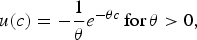
For analytical tractability, we assume that the utility function is represented by the following:
 $$u\lpar c\rpar = - {1 \over \theta} e^{-\theta c}\, \hbox{for} \theta \gt 0\comma \;$$
where θ denotes the Arrow–Pratt measure of absolute risk aversion. Furthermore, for ease of analysis, we assume that
 $\Psi \colon {\open R} \rightarrow {\open R}$
is linear. Then, the government's preferences represented by (4) turn out to be
$\Psi \colon {\open R} \rightarrow {\open R}$
is linear. Then, the government's preferences represented by (4) turn out to be
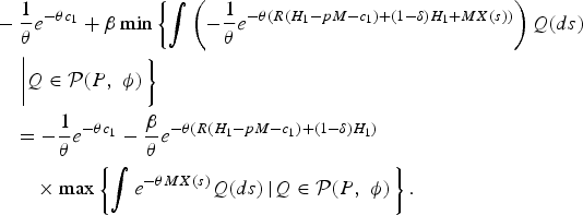 $$\eqalign{&-{1 \over \theta} e^{-\theta c_1} +\beta \min \left\{\vint \left(-{1 \over \theta} e^{-\theta \lpar R\lpar H_{1}-pM-c_{1}\rpar + \lpar 1-\delta\rpar H_{1} + MX\lpar s\rpar \rpar } \right)Q\lpar ds\rpar \right. \cr &\quad \left. \left\vert Q\in {\cal P}\lpar P\comma \; \phi\rpar \vphantom{\vint\left(-{1 \over \theta}e^{-\theta \lpar R\lpar H_{1}-pM-c_{1}\rpar + \lpar 1-\delta \rpar H_{1} + MX\lpar s\rpar \rpar }\right)}\right. \right\}\cr &\quad =-{1 \over \theta} e^{-\theta c_1} - {\beta \over \theta} e^{-\theta \lpar R\lpar H_{1}-pM-c_{1}\rpar + \lpar 1-\delta\rpar H_1\rpar } \cr &\qquad \times \max \left\{\vint e^{-\theta MX\lpar s\rpar } Q\lpar ds\rpar \left\vert Q\in {\cal P}\lpar P\comma \; \phi \rpar \right. \right\}.}$$
Note that
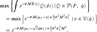 $$\eqalign{&\max \left\{\vint e^{-\theta MX\lpar s\rpar }Q\lpar ds\rpar \left\vert Q\in {\cal P}\lpar P\comma \; \phi\rpar \right. \right\}\cr &\quad = \max \left\{e^{-\theta M\lpar \mu_{x}-v\rpar + {1 \over 2}\theta^{2}M^{2}\sigma_{x}^{2}}\, \left\vert \, v\in {\cal V}\lpar \phi \rpar \right. \right\}\cr &\quad = e^{-\theta M\lpar \mu_{x} - \sqrt{2}\phi \sigma_{x}\rpar + {1 \over 2}\theta^{2}\sigma_{x}^{2}M^{2}}.}$$
Thus, the government's objective function is as follows:
 $$-{1 \over \theta}e^{-\theta c_1}- {\beta \over \theta}e^{-\theta \lpar R\lpar H_{1}-pM-c_{1}\rpar +\lpar 1-\delta\rpar H_1\rpar } \times e^{-\theta M\lpar \mu_{x}-\sqrt{2}\phi \sigma_{x}\rpar + {1 \over 2}\theta^{2}\sigma_{x}^{2}M^{2}}.$$
By the first-order condition with respect to consumption at t = 1, c 1, it follows that
 $$e^{-\theta c_{1}^{\ast}} = \beta R e^{-\theta \lpar R\lpar H_{1}-pM-c_{1}^{\ast }\rpar + \lpar 1-\delta\rpar H_1\rpar } \times e^{-\theta M\lpar \mu_{x}-\sqrt{2}\phi \sigma_{x}\rpar + {1 \over 2}\theta^{2}\sigma_{x}^{2}M^{2}}.$$
Then, the optimal consumption at t = 1, c 1*, is as follows:
 $$c_{1}^{\ast } = {R\lpar H_1 - pM\rpar + \lpar 1 - \delta\rpar H_1 \over 2} - {\ln \lpar \beta R\rpar \over 2\theta} + {\lpar \mu _{x}-\sqrt{2}\phi \sigma _{x}\rpar M \over 2} - {\theta \sigma_{x}^{2}M^{2} \over 4}.$$
Now, we are in a position to present the following proposition.
Proposition 1
The government's optimal natural capital investment is obtained as follows:
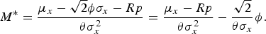 $$M^{\ast} = {\mu_{x} -\sqrt{2}\phi \sigma_{x}-Rp \over \theta \sigma_{x}^{2}} = {\mu_{x}-Rp \over \theta \sigma_{x}^{2}} - {\sqrt{2} \over \theta \sigma_{x}} \phi.$$
Proof: The optimal natural capital investment, M*, follows from the first-order condition with respect to the natural capital investment at t = 1, M:
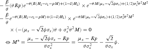 $$\eqalign{&-{\beta \over \theta}\lpar \theta Rp\rpar e^{-\theta\lpar R\lpar H_1-c_1-pM\rpar +\lpar 1-\delta\rpar H_1\rpar } \times e^{-\theta M\lpar \mu_x-\sqrt{2}\phi \sigma_x\rpar +\lpar 1/2\rpar \sigma_x^2 \theta^2 M^2} \cr &-{\beta \over \theta}e^{-\theta\lpar R\lpar H_1-c_1-pM\rpar +\lpar 1-\delta\rpar H_1\rpar } \times e^{-\theta M\lpar \mu_x-\sqrt{2}\phi \sigma_x\rpar +\lpar 1/2\rpar \sigma_x^2 \theta^2 M^2}\cr &\qquad \times \lpar -\lpar \mu_x-\sqrt{2}\phi \sigma_x\rpar \theta +\sigma_x ^2 \theta^2 M\rpar =0 \cr &\quad \Leftrightarrow M^{\ast} = {\mu_{x}-\sqrt{2}\phi \sigma _{x}-Rp \over \theta \sigma _{x}^{2}} = {\mu_{x}-Rp \over \theta \sigma_{x}^{2}} - {\sqrt{2} \over \theta \sigma_{x}} \phi.}$$
The interpretation of the first and second terms on the right-hand side of equation (5) is obvious. The first term captures risk in natural capital investment and the government's attitude toward risk. The second term, in contrast, captures the government's attitude toward ambiguity. Since we assume that ϕ, θ and σ x are all positive, the mere presence of ambiguity makes the government decrease its optimal natural capital investment as compared to the case in which there is no ambiguity; that is, ϕ = 0. Furthermore, the following proposition can be obtained.
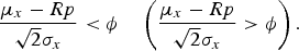
Proposition 2
The signs of the government's optimal natural capital investment are determined by the degree of ambiguity, ϕ. That is,
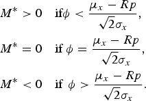 $$\eqalign{M^{\ast}& \gt 0 \quad \hbox{if} \phi \lt {\mu_{x}-Rp \over \sqrt{2}\sigma_{x}}\comma \; \cr M^{\ast} &= 0 \quad \hbox{if}\ \phi = {\mu _{x}-Rp \over \sqrt{2}\sigma_{x}}\comma \; \cr M^{\ast}& \lt 0 \quad \hbox{if }\, \phi \gt {\mu_{x}-Rp \over \sqrt{2}\sigma_{x}}.}$$
Proposition 2 states that the government makes a positive natural capital investment if the degree of ambiguity is sufficiently small. This is because low ambiguity regarding the effect of natural capital investment does not necessarily discourage such investment. On the other hand, the government makes a negative natural capital investment if the degree of ambiguity is sufficiently large, because high ambiguity about the associated effects discourages such investment. More specifically, the presence of ambiguity regarding the mean of the returns on natural capital investment leads the government to invest in the environment positively (negatively) only when the premium on natural capital investment, μ x − Rp, is sufficiently large (small). It is noteworthy that if there is no ambiguity, that is, if ϕ = 0, then the government's investment behavior determines only whether μ x > Rp, μ x = Rp or μ x < Rp.
It should be reiterated here that positive natural capital investment, translated into real terms, is equivalent to the government's activities to protect the environment, while negative natural capital investment is equivalent to the government's activities that destroy the environment. Proposition 2 means that when a government is faced with ambiguity under which the effects of investment in the environment cannot be foreseen, it might not hesitate to destroy the environment. We must hasten to add that Proposition 2 only shows that increases in ambiguity about effects of natural capital investment decrease the amount of natural capital investment; the results do not mean that increases in ambiguity about future events (for example, the potential threat of global warming) generally decrease the amount of natural capital investment. In fact, subsection 2.4 of this paper shows that, by reformulating our model, we can reach a situation where an increase in the ambiguity of future natural capital increases the optimal amount for natural capital investment. That is, the results obtained in this paper show that the results of comparative static analyses about ambiguity depend on the manner in which ambiguity is incorporated into the model.
The following proposition is derived from equation (5).
Proposition 3
An increase in ambiguity (that is, ϕ) decreases the optimal amount of natural capital investment (that is, M*).
Proof: This proposition is obtained from the following:
 $${\partial M^{\ast} \over \partial \phi} = - {\sqrt{2} \over \theta \sigma_x}.$$
The interpretation of this result is clear. It is obtained because an increase in ambiguity makes the government more cautious about the effect of natural capital investment and makes it hesitant to invest in the environment. The larger the degree of ambiguity (that is, ϕ ), the larger the government's set of beliefs (that is,
 ${\cal P}\lpar P\comma \; \phi \rpar $
), which makes the government more cautious about the effect of natural capital investment. Therefore, the government is less likely to invest in natural capital.
${\cal P}\lpar P\comma \; \phi \rpar $
), which makes the government more cautious about the effect of natural capital investment. Therefore, the government is less likely to invest in natural capital.
As the following proposition states, the effect of ambiguity on the optimal amount of consumption depends on the degree of ambiguity.
Proposition 4
An increase in ambiguity increases (decreases) the optimal amount of consumption (that is, c 1*) if the degree of ambiguity is sufficiently large (small); that is,
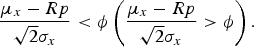 $${\mu_x -Rp \over \sqrt{2}\sigma_x} \lt \phi \left({\mu_x -Rp \over \sqrt{2} \sigma_x} \gt \phi \right).$$
Proof: This proposition is obtained from the following:
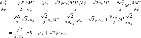 $$\eqalign{{\partial c_1^{\ast} \over \partial \phi} &= -{pR \over 2}{\partial M^{\ast} \over \partial \phi}+ {\lpar \mu_x -\sqrt{2} \phi \sigma_x\rpar \partial M^{\ast}/\partial \phi - \sqrt{2} \sigma_x M^{\ast} \over 2} - {\theta \sigma_x ^2 \over 2}M^{\ast} {\partial M^{\ast} \over \partial \phi} \cr &= {pR \over 2} {\sqrt{2}}{\theta \sigma_x}- {\sqrt{2} \over 2} \sigma_x M^{\ast} -{\sqrt{2} \over 2 \theta \sigma_x}\lpar \mu_x -\sqrt{2} \phi \sigma_x\rpar +{\theta \sigma_x ^2 \over 2} M^{\ast} {\sqrt{2} \over \theta \sigma_x} \cr &= {\sqrt{2} \over 2 \theta \sigma_x}\lpar pR - \mu_x + \sqrt{2} \phi \sigma_x\rpar \comma \; }$$
where the second equation holds by equation (6).
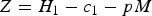
Next, we analyze the effect of ambiguity on the optimal amount of saving, Z* = H 1 − c 1* − pM*.
Proposition 5
An increase in ambiguity increases the optimal amount of saving if the degree of ambiguity is sufficiently small; that is,
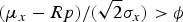 $\lpar \mu_{x}-Rp\rpar /\lpar \sqrt{2}\sigma_{x}\rpar \gt \phi$
.
$\lpar \mu_{x}-Rp\rpar /\lpar \sqrt{2}\sigma_{x}\rpar \gt \phi$
.
Proof: This proposition is obtained from the following:
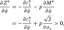 $$\eqalign{{\partial Z^{\ast} \over \partial \phi} &= -{\partial c_1 ^{\ast} \over \partial \phi}-p{\partial M^{\ast} \over \partial \phi} \cr &=-{\partial c_1 ^{\ast} \over \partial \phi}+p{\sqrt{2} \over \theta \sigma_x} \gt 0\comma \; }$$
where the second equation follows from equation (6) and Proposition 4.
This proposition corresponds to the notion of precautionary saving in the asset pricing literature, which states that an increase in ambiguity leads to more saving.
Finally, we analyze the effects of increases in the degree of risk aversion on the optimal amount of natural capital investment. The following proposition states that these effects depend on the degree of ambiguity.
Proposition 6
An increase in the degree of risk aversion (that is, θ) increases (decreases) the optimal amount of natural capital investment (that is, M*) if the degree of ambiguity is sufficiently large (small); that is, if
 $${\mu_x -Rp \over \sqrt{2} \sigma_x} \lt \phi\quad \left({\mu_x -Rp \over \sqrt{2} \sigma_x} \gt \phi \right).$$
Some comments are in order. The sufficient conditions in Proposition 6 correspond to those in Proposition 2. If the degree of ambiguity is sufficiently large (small), then not only is the optimal natural capital investment, M*, negative (positive), but also an increase in the degree of risk aversion increases (reduces) such investment. This proposition means that if the degree of risk aversion increases, then the presence of ambiguity about the effect of natural capital investment makes the government cautious about such investment in a positive or a negative direction. This proposition also implies that the government's degree of risk aversion alone does not necessarily provide a clue to likely environmental policies: the degree of ambiguity should also be considered. Of course, if there is no ambiguity, that is, if ϕ = 0, then an increase in the degree of risk aversion increases (decreases) the optimal natural capital investment only when the premium on natural capital investment, μ x − Rp, is negative (positive).
2.2.2. Quadratic cost function
Next, we analyze the case in which the effect of natural capital investment is uncertain and the return from saving is deterministic. In addition, we assume that the government's cost function is quadratic. In this case, the government's objective function represented by (4) becomes
 $$\eqalign{&-{1 \over \theta}e^{-\theta c_{1}}+\beta \min \left\{\vint \left(-{1 \over \theta }e^{-\theta \lpar R\lpar H_{1}-\lpar 1/2\rpar pM^2-c_{1}\rpar +\lpar 1-\delta\rpar H_{1}+MX\lpar s\rpar \rpar }\right)Q\lpar ds\rpar \right. \cr &\qquad \left. \vphantom{\vint \left(-{1 \over \theta}e^{-\theta \lpar R\lpar H_{1}-\lpar 1/2\rpar pM^2-c_{1}\rpar +\lpar 1-\delta\rpar H_{1}+MX\lpar s\rpar \rpar }\right)}\left\vert Q\in {\cal P}\lpar P\comma \; \phi\rpar \right. \right\}\cr &\quad =-{1 \over \theta} e^{-\theta c_1} - {\beta \over \theta}e^{-\theta \lpar R\lpar H_{1}-\lpar 1/2\rpar pM^2-c_{1}\rpar +\lpar 1-\delta\rpar H_1\rpar }\cr &\qquad \times \max \left\{\vint e^{-\theta MX\lpar s\rpar }Q\lpar ds\rpar \left\vert Q\in {\cal P}\lpar P\comma \; \phi \rpar \right. \right\}\cr &\quad = -{1 \over \theta} e^{-\theta c_{1}}-{\beta \over \theta }e^{-\theta \lpar R\lpar H_{1}-\lpar 1/2\rpar pM^2-c_{1}\rpar +\lpar 1-\delta\rpar H_1\rpar }\cr &\quad \times e^{-\theta M\lpar \mu_x -\sqrt{2}\phi \sigma_x\rpar +\lpar 1/2\rpar \sigma_x ^2 \theta^2 M^2}.}$$
By the first-order condition with respect to M, it follows that
 $$\eqalign{&-{\beta \over \theta}\lpar \theta R p M\rpar e^{-\theta\lpar R\lpar H_1-c_1-\lpar 1/2\rpar pM^2\rpar +\lpar 1-\delta\rpar H_1\rpar } \times e^{-\theta M\lpar \mu_x -\sqrt{2}\phi \sigma_x\rpar +\lpar 1/2\rpar \sigma_x ^2 \theta^2 M^2} \cr &-{\beta \over \theta}e^{-\theta\lpar R\lpar H_1 -c_1-\lpar 1/2\rpar pM^2\rpar +\lpar 1-\delta\rpar H_1\rpar } \times e^{-\theta M\lpar \mu_x -\sqrt{2}\phi \sigma_x\rpar +\lpar 1/2\rpar \sigma_x ^2 \theta^2 M^2} \cr &\qquad \times \lpar -\theta\lpar \mu_x -\sqrt{2} \phi \sigma_x\rpar +\sigma_x ^2 \theta^2 M\rpar =0.}$$
Then, the optimal amount of natural capital investment is derived as follows:
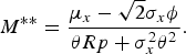 $$M^{\ast \ast} = {\mu_x -\sqrt{2} \sigma_x \phi \over \theta R p +\sigma_x ^2 \theta^2}.$$
By equation (7), we obtain
 $\partial M^{\ast \ast }/\partial \phi =-\lpar \sqrt{2}\sigma _{x}\rpar /\lpar \theta Rp+\sigma_{x}^{2}\theta ^{2}\rpar \lt 0$
, which corresponds to Proposition 3. Therefore, the effect of ambiguity on the amount of natural capital investment is not altered if the cost function is assumed to be quadratic.
$\partial M^{\ast \ast }/\partial \phi =-\lpar \sqrt{2}\sigma _{x}\rpar /\lpar \theta Rp+\sigma_{x}^{2}\theta ^{2}\rpar \lt 0$
, which corresponds to Proposition 3. Therefore, the effect of ambiguity on the amount of natural capital investment is not altered if the cost function is assumed to be quadratic.
2.3. Ambiguity about natural capital dynamics
In this subsection, we reformulate the simple two-period natural capital investment model under Knightian uncertainty analyzed in subsection 2.2 in order to shed light on the government's optimal natural investment from a different viewpoint. Contrary to subsection 2.2, in which the effect of natural capital investment is uncertain and the return from saving is deterministic, in this subsection, we assume that the former is deterministic and the latter is uncertain. That is, the return from saving,
 $R\colon S\rightarrow {\open R}$
, is normally distributed with mean μ
r
and variance σ
r
.Footnote
10
$R\colon S\rightarrow {\open R}$
, is normally distributed with mean μ
r
and variance σ
r
.Footnote
10
As in subsection 2.1, let P be the reference probability corresponding to a normal distribution with mean μ
r
and variance σ
r
2. It is assumed that all of the government's beliefs in
 ${\cal P}\lpar P\comma \; \phi \rpar $
, as defined by (2), have normal distributions. Each probability measure in
${\cal P}\lpar P\comma \; \phi \rpar $
, as defined by (2), have normal distributions. Each probability measure in
 ${\cal P}\lpar P\comma \; \phi \rpar $
has variance σ
r
and mean μ
r
− v for some
${\cal P}\lpar P\comma \; \phi \rpar $
has variance σ
r
and mean μ
r
− v for some
 $v\in {\open R}$
. As we explain in subsection 2.1,
$v\in {\open R}$
. As we explain in subsection 2.1,
 ${\cal P} \lpar P\comma \; \phi \rpar $
is isomorphic to
${\cal P} \lpar P\comma \; \phi \rpar $
is isomorphic to
 ${\cal V}\lpar \phi \rpar $
, which is defined by (3).
${\cal V}\lpar \phi \rpar $
, which is defined by (3).
The government's problem can thus be rewritten as follows. The government is supposed to choose c 1 and M in order to maximize the following objective function:
 $$u\lpar c_{1}\rpar +\beta \min \left\{\vint u\lpar c_{2}\rpar Q\lpar ds\rpar \left\vert Q\in {\cal P}\lpar P\comma \; \phi \rpar \right. \right\}.$$
In this subsection, since we assume that the return from saving, R, is uncertain,
 $c_{2}=\lpar \Psi\lpar H_{1}\rpar -pM-c_{1}\rpar R\lpar s\rpar +\Psi\lpar H_{2}\rpar $
. For analytical tractability, we assume that the utility function is represented as follows:
$c_{2}=\lpar \Psi\lpar H_{1}\rpar -pM-c_{1}\rpar R\lpar s\rpar +\Psi\lpar H_{2}\rpar $
. For analytical tractability, we assume that the utility function is represented as follows:
 $$u\lpar c\rpar =-{1 \over \theta }e^{-\theta c}\, \hbox{for}\, \theta \gt 0\comma \;$$
where θ denotes the Arrow–Pratt measure of absolute risk aversion. Furthermore, for ease of analysis, we assume that
 $\Psi \colon {\open R} \rightarrow {\open R}$
is linear.
$\Psi \colon {\open R} \rightarrow {\open R}$
is linear.
The government's objective function turns out to be
 $$\eqalign{&-{1 \over \theta} e^{- \theta c_1}+\beta \min \left\{\vint \left(-{1 \over \theta}e^{-\theta\lpar R\lpar s\rpar \lpar H_1-c_1-pM\rpar +\lpar 1-\delta\rpar H_1+XM\rpar } \right)Q\lpar ds\rpar \right.\cr &\qquad \left.\vphantom{\left(-{1 \over \theta}e^{-\theta\lpar R\lpar s\rpar \lpar H_1-c_1-pM\rpar +\lpar 1-\delta\rpar H_1+XM\rpar } \right)} \bigg\vert \, Q \in {\cal P}\lpar P\comma \; \phi\rpar \right\}\cr &\quad = -{1 \over \theta} e^{- \theta c_1} -{\beta \over \theta} e^{-\theta\lpar \lpar 1-\delta\rpar H_1+XM\rpar }\cr &\qquad \times \max \left\{\vint e^{-\theta Z R\lpar s\rpar } Q\lpar ds\rpar \, \bigg\vert \, Q \in {\cal P}\lpar P\comma \; \phi\rpar \right\}\cr &\quad = -{1 \over \theta} e^{- \theta c_1} -{\beta \over \theta} e^{-\theta\lpar \lpar 1-\delta\rpar H_1+XM\rpar } \times e^{-\theta Z \lpar \mu_r-\sqrt{2} \phi \sigma_r\rpar +\lpar 1/2\rpar \sigma_r^2 \theta^2 Z^2}\comma \; }$$
where
 $Z=H_{1}-c_{1}-pM$
. Then, the following proposition is in order.
$Z=H_{1}-c_{1}-pM$
. Then, the following proposition is in order.
Proposition 7
The optimal amount of the government's natural capital investment is obtained as follows:
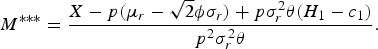 $$M^{\ast \ast \ast} = {X-p\lpar \mu_r-\sqrt{2} \phi \sigma_r\rpar +p \sigma_r ^2 \theta \lpar H_1-c_1\rpar \over p^2 \sigma_r ^2 \theta}.$$
Proof: The optimal natural capital investment, M ***, follows from the first-order condition with respect to the natural capital investment at t = 1,M:
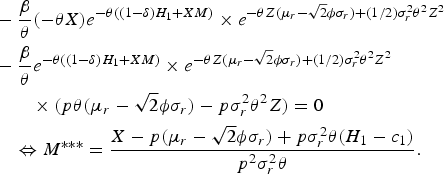 $$\eqalign{& -{\beta \over \theta}\lpar -\theta X\rpar e^{-\theta\lpar \lpar 1-\delta\rpar H_1+XM\rpar } \times e^{-\theta Z\lpar \mu_r-\sqrt{2}\phi \sigma_r\rpar +\lpar 1/2\rpar \sigma_r ^2 \theta^2 Z ^2} \cr &-{\beta \over \theta} e^{-\theta\lpar \lpar 1-\delta\rpar H_1+XM\rpar }\times e^{-\theta Z\lpar \mu_r-\sqrt{2}\phi \sigma_r\rpar +\lpar 1/2\rpar \sigma_r ^2 \theta^2 Z ^2} \cr &\qquad \times \lpar p\theta\lpar \mu_r-\sqrt{2}\phi \sigma_r\rpar -p\sigma_r ^2 \theta^2 Z\rpar =0 \cr &\quad \Leftrightarrow M^{\ast \ast \ast} = {X-p\lpar \mu_r-\sqrt{2} \phi \sigma_r\rpar +p \sigma_r ^2 \theta \lpar H_1-c_1\rpar \over p^2 \sigma_r ^2 \theta}.}$$
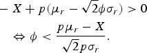
Proposition 8
The signs of the government's optimal natural capital investment are determined by the degree of ambiguity, ϕ. That is,
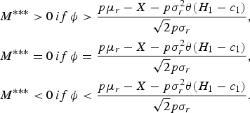 $$\eqalign{M^{\ast \ast \ast} \gt 0 &\, {if}\, \phi \gt {p \mu_r-X-p\sigma_r ^2 \theta \lpar H_1-c_1\rpar \over \sqrt{2} p\sigma_{r}}\comma \; \cr M^{\ast \ast \ast}=0 &\, {if}\, \phi = {p \mu_r-X-p\sigma_r ^2 \theta \lpar H_1-c_1\rpar \over \sqrt{2} p\sigma_{r}}\comma \; \cr M^{\ast \ast \ast} \lt 0 &\, {if}\, \phi \lt {p \mu_r-X-p\sigma_r ^2 \theta \lpar H_1-c_1\rpar \over \sqrt{2} p\sigma_{r}}.}$$
Proposition 8 is the opposite of Proposition 2. Proposition 2 states that the government makes a positive (negative) natural capital investment if the degree of ambiguity is sufficiently small (large). In contrast, Proposition 8 states that the government makes a positive (negative) natural capital investment if the degree of ambiguity is sufficiently large (small). The difference between Proposition 2 and Proposition 8 stems from the way in which ambiguity is incorporated into the models.
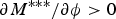
Let us next analyze the effect of ambiguity on the optimal natural capital investment. Contrary to Proposition 3, which states that an increase in ambiguity decreases the optimal natural capital investment, the following proposition states that an increase in ambiguity increases the optimal natural capital investment.
Proposition 9
An increase in ambiguity (that is, ϕ) increases the optimal amount of natural capital investment (that is, M***) if the degree of ambiguity is sufficiently small, that is,
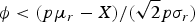 $\phi \lt \lpar p\mu_{r}-X\rpar /\lpar \sqrt{2} p \sigma_{r}\rpar $
.
$\phi \lt \lpar p\mu_{r}-X\rpar /\lpar \sqrt{2} p \sigma_{r}\rpar $
.
Proof: By differentiating M *** with respect to ϕ, it follows that
 $${\partial M^{\ast \ast \ast} \over \partial \phi}={1 \over p^2 \sigma_r ^2 \theta}\left(\sqrt{2}p\sigma_r -p \sigma_r ^2 \theta {\partial c_1 \over \partial \phi} \right).$$
By the first-order condition with respect to c 1, it follows that
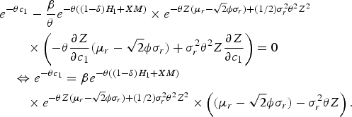 $$\eqalign{& e^{-\theta c_1} -{\beta \over \theta} e^{-\theta\lpar \lpar 1-\delta\rpar H_1+XM\rpar } \times e^{-\theta Z \lpar \mu_r-\sqrt{2}\phi \sigma_r\rpar +\lpar 1/2\rpar \sigma_r ^2 \theta^2 Z^2}\cr &\qquad \times \left(-\theta {\partial Z \over \partial c_1}\lpar \mu_r-\sqrt{2}\phi \sigma_r\rpar +\sigma_r ^2 \theta^2 Z {\partial Z \over \partial c_1} \right)=0 \cr &\quad \Leftrightarrow e^{-\theta c_1}=\beta e^{-\theta\lpar \lpar 1-\delta\rpar H_1+XM\rpar }\cr &\qquad \times e^{-\theta Z \lpar \mu_r-\sqrt{2}\phi \sigma_r\rpar +\lpar 1/2\rpar \sigma_r ^2 \theta^2 Z^2} \times \left(\lpar \mu_r -\sqrt{2}\phi \sigma_r\rpar -\sigma_r ^2 \theta Z \right).}$$
From equation (8), we obtain the following:
 $${\partial M^{\ast \ast \ast} \over \partial \phi}+{1 \over p}{\partial c_1^{\ast \ast \ast} \over \partial \phi} = {\sqrt{2} \over p \sigma_r \theta}.$$
Several lines of calculation yield
 $${\partial c_1^{\ast \ast \ast} \over \partial \phi} = -{\sqrt{2}\lpar -X+p\lpar \mu_r -\sqrt{2}\phi \sigma_r\rpar \rpar \over \theta \lpar p+X\rpar \sigma_r}.$$
The sign of
 $\partial c_{1} ^{\ast \ast \ast}/\partial \phi$
is negative if
$\partial c_{1} ^{\ast \ast \ast}/\partial \phi$
is negative if
 $$\eqalign{&-X+p\lpar \mu_r -\sqrt{2} \phi \sigma_r\rpar \gt 0 \cr &\quad \Leftrightarrow\phi \lt {p\mu_r-X \over \sqrt{2} p \sigma_r}.}$$
If Condition (11) holds, then it follows from (8) that
 $\partial M^{\ast \ast \ast} / \partial \phi \gt 0$
.
$\partial M^{\ast \ast \ast} / \partial \phi \gt 0$
.
This result is in stark contrast to Proposition 3. This proposition, when considered together with Proposition 3, means that not only does the degree of ambiguity affect the government's natural capital investment but also that the direction of the effect of the ambiguity depends on the way ambiguity is incorporated into the model.
Finally, we analyze the effect of ambiguity on the optimal amount of saving,
 $Z^{\ast \ast \ast} = H_{1}-c_{1}^{\ast \ast \ast} -pM^{\ast \ast \ast}$
.
$Z^{\ast \ast \ast} = H_{1}-c_{1}^{\ast \ast \ast} -pM^{\ast \ast \ast}$
.
Proposition 10
An increase in ambiguity decreases the optimal amount of saving.
Proof: This proposition is obtained from the following:
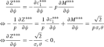 $$\eqalign{&{\partial Z^{\ast \ast \ast} \over \partial \phi} = - {\partial c_1 ^{\ast \ast \ast} \over \partial \phi} - p {\partial M^{\ast \ast \ast} \over \partial \phi} \cr \Leftrightarrow &-{1 \over p} {\partial Z^{\ast \ast \ast} \over \partial \phi} = {1 \over p}{\partial c_1 ^{\ast \ast \ast} \over \partial \phi}+{\partial M^{\ast \ast \ast} \over \partial \phi}= {\sqrt{2} \over p \sigma_r \theta} \cr \Leftrightarrow&{\partial Z^{\ast \ast \ast} \over \partial \phi}=-{\sqrt{2} \over \sigma_r \theta} \lt 0\comma \; }$$
where the first and the second equations of the first equivalence follow from equation (9) and equation (10), respectively.
This proposition is in contrast with Proposition 5. Proposition 5 states that an increase in ambiguity (that is, ϕ ) leads to more saving for a sufficiently small ϕ, which corresponds to the standard precautionary saving result in the literature on consumption. On the other hand, Proposition 10 states that an increase in ambiguity leads to less saving, which does not depend on the degree of ambiguity, ϕ.
3. Conclusion
Within a simple two-period model, we derived the optimal amount of natural capital investment under Knightian uncertainty and analyzed the way in which the degree of such uncertainty affects the optimal investment. Moreover, we showed that the degree of Knightian uncertainty and that of risk aversion determine whether a government makes a positive, negative, or zero natural capital investment and that an increase in this uncertainty affects the optimal amount of such investment. The results obtained by this study suggest that ambiguity regarding environmental policy efficacy could make a government hesitant to adopt policies intended, for example, to reduce CO 2 emissions or protect endangered species, owing to a lack of clarity about their likely effects. At the same time, however, the results also show that the effect of an increase in ambiguity on natural capital investment depends on the way in which ambiguity is incorporated into the model. A significant policy implication of this paper is that we must consider both the degree and the nature of ambiguity. In other words, we must consider whether the ambiguity is regarding the future level of natural capital or about the return from saving.
Finally, our work has certain limitations. First, in analyzing the effects of uncertainty, we assumed that uncertainty is captured by normal distributions. However, this assumption might be restrictive. Second, in general, the externalities associated with environmental capital are not included in the definition of GDP. However, we assumed that the government is able to internalize all such externalities. These two simplifying assumptions enabled us to derive analytical solutions and to perform comparative static analyses. Hence, relaxing these assumptions would be an important research topic.