2. The economic valuation of air pollution

According to Rosen's (Reference Rosen1974) seminal paper, final housing prices can be empirically assessed as a function of their structural and site-specific attributes. A few years later, these local attributes represented the key inputs for modeling cross-city differences in housing prices under a spatial equilibrium framework (Rosen, Reference Rosen, Mieszkowski and Strashaim1979; Roback, Reference Roback1982). Under this model, individuals choose their locations to maximize their utility. In so doing, they sort across cities according to their preferences, reaching spatial equilibrium, where there are no utility differences across space for workers with identical preferences and skills (Winters, Reference Winters2009).

As Ferreira and Moro (Reference Ferreira and Moro2010) assert, under the spatial equilibrium approach, researchers may follow three alternative empirical methods to value environmental (dis)amenities. The first two methods are the stated-preference and life satisfaction approaches. The latter is relatively novel compared with the former, and it directly estimates the effects of an amenity on individual subjective wellbeing – which acts as a proxy for individuals’ utility – to compute the marginal willingness to pay for improvements in environmental attributes.Footnote ³ However, this study follows the third approach – the traditional revealed preference approach – using a hedonic equation to assess the effects of PM_2.5 concentration on housing rental prices.

In what follows, we present the main characteristics of the hedonic model following Freeman et al. (Reference Freeman, Herriges and Kling2014) and Carriazo and Gomez-Mahecha (Reference Carriazo and Gomez-Mahecha2018). Under this model, a household's utility function may be represented as $U(x,\; \boldsymbol{Q})$, where x is a composite good and $\boldsymbol{Q}$ is a vector of the characteristics that affect housing rental price, such as housing, neighborhood, and commune attributes (including PM_2.5 concentration). If the housing market is in equilibrium, the housing rental price can be represented as $P(\boldsymbol{Q})$. This expression is reminiscent of the well-known hedonic equation, in which housing rental price depends on a vector of attributes $\boldsymbol{Q}$.

In equilibrium, a household chooses the optimal level of the attribute that maximizes its utility, subject to the budget constraint $M = \boldsymbol{x} + P(\boldsymbol{Q})$. Since the price of x is 1, the optimal consumption of attribute ${q_1}$ is reached where the marginal rate of substitution between the attribute and composite good equals the implicit price of the attribute – that is, $((\partial U/\partial {q_1})/(\partial U/\partial x)) = ((\partial P(\boldsymbol{Q}))/\partial {q_1})$. Importantly, using this condition, an expression for the marginal willingness to pay (MWTP) might be found for changes in the ${q_1}$ attribute (e.g., PM_2.5). For a log-linear hedonic function, this can be computed as:

(1)\begin{equation}\frac{{\partial P(\boldsymbol{Q})}}{{\partial {q_1}}} = \textrm{MWT}{\textrm{P}_{{q_1}}} = {\hat{\beta }_{{q_1}}}P,\end{equation}

where $\hat{\beta }$ is the estimated coefficient for attribute ${q_1}$ of the hedonic equation. As stressed by Freeman et al. (Reference Freeman, Herriges and Kling2014), it is important to bear in mind that equation (1) only allows estimation of the household's MWTP for small changes in ${q_1}$, keeping the utility level constant. This expression, however, does not provide the function itself. The estimation found via equation (1) makes up ‘first stage studies,’ while empirical research aimed at estimating the willingness to pay function are known as ‘second stage studies.’ The estimation of the willingness to pay function is useful for performing welfare analyses to measure, for example, how welfare is modified under different scenarios of air pollution (e.g., Carriazo and Gomez-Mahecha, Reference Carriazo and Gomez-Mahecha2018), which is particularly relevant from a policy perspective.Footnote ⁴

The main motivation behind using first stage studies in this research is to perform welfare analysis to account for marginal changes in air pollution. As mentioned, this task differs from second stage studies which may compute welfare effects of non-marginal changes in air quality. In this context, since air pollution dampens the wellbeing of residents (i.e., an environmental (dis)amenity), the empirical first stage hedonic equation should reveal the negative effect of air pollution on housing rental prices.

The use of the housing market to assess the impact of environmental attributes has a long tradition in the empirical literature. From the pioneering study developed by Ridker and Henning (Reference Ridker and Henning1967) for the St. Louis metropolitan area, to the analyses of Davis (Reference Davis2011) and Currie et al. (Reference Currie, Davis, Greenstone and Walker2015), who study the impact of power plants and industrial plants on housing values in the United States, numerous scholars have used housing markets to infer the value of environmental amenities. The economic assessment of air pollution has followed this pattern – as noted by Smith and Huang (Reference Smith and Huang1995), who have performed a meta-analysis of 37 studies on air particulate matter and housing values in the United States between 1967 and 1988, and, more recently, by Yusuf and Resosudarmo (Reference Yusuf and Resosudarmo2009), who incorporate additional hedonic studies, including Seoul and Taipei.

Evidently, the extant body of literature keeps providing new empirical studies. However, while research among developed economies and China is plentiful,Footnote ⁵ empirical analyses of air pollution in Latin American countries, aside from Chile, are limited to only a few studies for México and Colombia. For México, scholars have studied PM₁₀ concentrations across states (Rodríguez-Sánchez, Reference Rodríguez-Sánchez2014) and, more recently, attention has been paid to México City with two studies: Chakraborti et al. (Reference Chakraborti, Heres and Hernandez2019), who analyze four air pollutants (PM₁₀, PM₂₅, SO₂, O₃) and Fontenla et al. (Reference Fontenla, Goodwin and Gonzalez2019), who only focus on PM₁₀ in México City. In Colombia, Carriazo et al. (Reference Carriazo, Ready and Shortle2013) and Carriazo and Gomez-Mahecha (Reference Carriazo and Gomez-Mahecha2018) analyze air pollution in Bogota. Both studies focus on PM₁₀ and, while the former employs a stochastic frontier model to address omitted variable bias, the latter estimates the second stage hedonic model to identify the demand function for PM₁₀ reduction. These studies, besides using different methodological approximations and air pollutants, confirm the negative effect of air pollution on residents’ quality of life.

3. Study case, interpolation, and data

3.2 Air pollution interpolation

As mentioned above, this study expands the geographical scope of current research by analyzing 312 communes. To accomplish this, it employs spatial interpolation to predict PM_2.5 concentration for communes without a monitoring station. This process involves two stages. First, PM_2.5 levels have been obtained from the National Air Quality Information System (SINCA, in its Spanish acronym) for 47 monitoring stations with valid data for 2017, distributed across 41 communes. As figure A1 in the online appendix shows, although monitoring stations are distributed along the whole territory, they are overrepresented in and around the Metropolitan Region in the middle of Chile.

Second, to predict missing commune levels of PM_2.5, we employ ordinary kriging techniques. Although there seems to be no consensus about whether, in general, the kriging method provides more reliable results compared to other techniques, it is recommended over inverse distance weighting – the other common interpolation technique – because of its precision and model fit (Naoum and Tsanis, Reference Naoum and Tsanis2004; Anselin and Le Gallo, Reference Anselin and Le Gallo2006; Brereton et al., Reference Brereton, Moro, Ningal and Ferreira2011).

The prediction derived from ordinary kriging results from a linear combination of observed points using a weight structure (Xie et al., Reference Xie, Chen, Lei, Yang, Guo, Song and Zhou2011). A general formula can be expressed as follows:

\[\hat{Z}({c_0}) = \mathop \sum \limits_{i = 1}^N {w_i}Z({c_i}),\]

where $\hat{Z}({c_0})$ represents the predicted PM_2.5 concentration in commune ${c_0}$; N corresponds to the monitoring stations; $Z({c_i})$ is the observed value in commune i; and ${w_i}$ is the weights. The derivation of weights represents the key difference between kriging and other methods because these weights are determined with the objective of minimizing variance (Oliver and Webster, Reference Oliver and Webster1990).

Figure 1 displays a map with the interpolated PM_2.5 concentrations for Chilean communes. The highest levels of air pollution are in the middle of Chile and in the southern communes. As previously mentioned, poor air quality in these communes is related to urban transportation, topographic conditions, and wood burning. In the upper-left corner of figure 1, a graph displays regional interpolated values sorted according to their geographical position. This confirms that the highest values are found in the Metropolitan Region of Santiago and in the southern regions of Araucanía, Los Rios, Los Lagos, and Aysén. These regions contain the nine most polluted Chilean communes, according to the 2018 World Air Quality Report; therefore, this result provides suggestive evidence to support the accuracy of our interpolated measures.

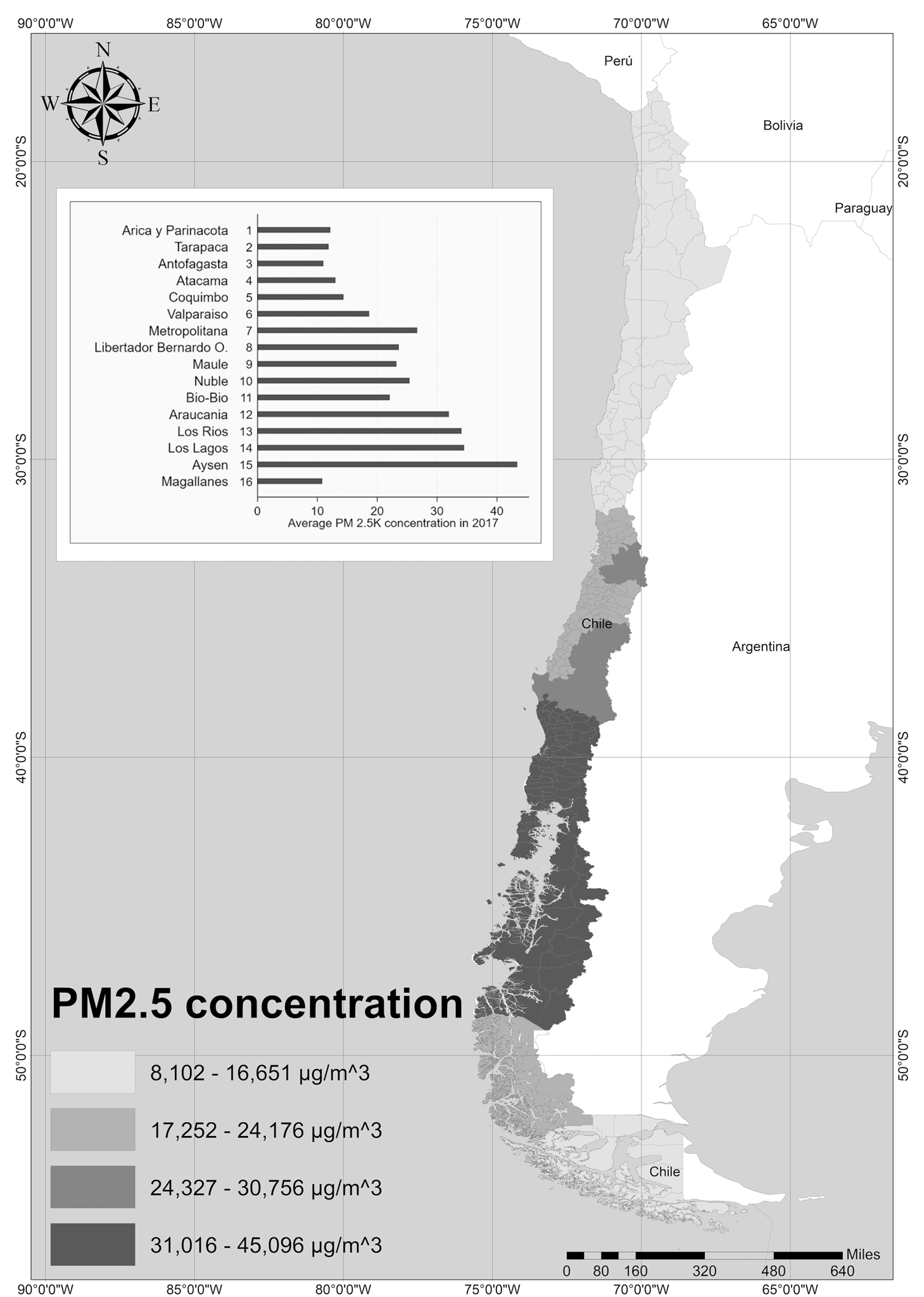
Figure 1. Interpolated commune PM_2.5 concentration.

Source: Authors’ own elaboration

3.3 Data

This study's main dataset comes from the Chilean National Socioeconomic Characterization Survey (CASEN) for 2017. This survey contains detailed information on housing characteristics, such as monthly housing rental prices, quality indexes, numbers of bathrooms, numbers of bedrooms, and square meters. From the total sample, we selected single-family households with a positive imputed rental price.Footnote ⁶ After handling missing values, the final sample corresponded to 49,649 dwellings distributed across 312 urban communes.Footnote ⁷

To control for neighborhood characteristics, the ideal scenario would be to have the specific spatial location of housing within each commune. The CASEN, however, does not offer such data. Rather, it asks respondents (using categorical questions) to provide information about how close their houses are to a set of services, such as public transport, educational centers, and supermarkets. Additionally, other questions capture residents’ perceptions regarding delinquency and pollution in their neighborhoods. In moving forward to commune-level attributes, we have controlled for natural sanctuaries (natural amenities) and a group of urban (dis)amenities, such as population density, typical places, cultural supply,Footnote ⁸ homicide rate, and the key independent variable of PM_2.5 concentration.Footnote ⁹

In addition to these control variables, it is important to highlight that the spatial distribution of air pollution closely relates to several (omitted) local activities, which also affect housing rental prices, such as local economic activity (e.g., industry and transportation), as stressed by Bayer et al. (Reference Bayer, Keohane and Timmins2009). Although the identification strategy will be addressed below, to begin mitigating omitted variable bias, we have taken advantage of satellite data, using nighttime light intensity as a proxy for communal economic activity (Donaldson and Storeygard, Reference Donaldson and Storeygard2016). As noted by Henderson et al. (Reference Henderson, Storeygard and Weil2012), the use of light increases as consumption and investment rise; therefore, light can be a proper measure of economic activity. To construct this variable, following the precedent of Soto et al. (Reference Soto, Vargas and Berdegué2018), we sum nighttime light within communal urban boundaries via the Visible Infrared Imaging Radiometer Suite (VIIRS) Day/Night Band (DBN), which has several advantages over previous light data used by researchers in different fields, as noticed by Elvidge et al. (Reference Elvidge, Kimberly, Mikhail, Feng and Tilottama2017). Table 1 displays the set of variables, as well as their descriptions, sources, and summary statistics.

Table 1. Definition of variables, sources, and summary statistics

Note: All variables correspond to 2017.

4. Econometric strategy

To assess the effects of air pollution on housing rental prices, we estimate the following empirical model:

(2)\begin{equation}\ln {p_{ij}} = \alpha + \beta {X_{ij}} + \gamma \textrm{PM}{2.5_j} + \theta {Z_j} + {\varepsilon _{ij}},\end{equation}

where the dependent variable is the natural log of the monthly housing rental price of dwelling i located in commune j. Vector X includes housing and neighborhood characteristics, while Z is a vector of commune-level variables, and $\varepsilon$ is the residuals. The parameter of interest in this case is $\gamma$, which measures the marginal effect of PM_2.5 on the log of housing rental price.

The estimation of equation (2) will provide a mere adjusted statistical association between PM_2.5 and a log of housing rental price. To reliably approximate the causal effect, two empirical challenges must be faced. First, as recognized by Anselin (Reference Anselin2001), interpolation methods are associated with measurement errors, which means that the true level of air pollution is measured with errors. In the regression analysis, these errors are captured by the residuals which produces measurement error bias in the parameter of interest. Additionally, as suggested in the previous section, omitted variable bias also represents a serious concern because commune levels of air pollution are closely related to unobserved local conditions contained in the residuals such as industrial activity and traffic congestion which, in turn, are positively associated with both housing rental prices and air pollution (Bayer et al., Reference Bayer, Keohane and Timmins2009). This results in an upward biased ordinary least squares (OLS) estimate, making the estimated coefficient show a smaller negative effect than it should.Footnote ¹⁰

To handle endogeneity concerns, we follow an instrumental variables approach. We must, then, find an instrument meeting two conditions. It must be correlated with the endogenous variable (relevance), and it must be orthogonal to the error term (exclusion). We partially follow the identification strategy proposed by Bayer et al. (Reference Bayer, Keohane and Timmins2009), which employs pollution sources across US counties to create an exogenous local shock for each county. To the best of the authors’ knowledge, although Chile has detailed information about PM_2.5 emissions, unlike the US context, it does not have a matrix reflecting pollution transmission across communes. To overcome this issue, following the precedent of Rodríguez-Sánchez (Reference Rodríguez-Sánchez2014), this research takes a simple approach, by computing, for each commune, the weighted sum of the PM_2.5 emissions (in tons) from communes farther away than 100 km but nearer than 500 km:Footnote ¹¹

(3)\begin{equation}{E_c} = \mathop \sum \limits_j \frac{{\textrm{PM}{{2.5}_j}}}{{{d_{cj}}}}\end{equation}

The total emissions $(E)$ affecting commune c is the sum of the emissions of all communes j, located farther than 100 km away but nearer than 500 km $(100 < {d_{cj}} < 500)$. We also create another instrument by applying equation (3), restricting it to communes farther than 500 km away. As shown by Li et al. (Reference Li, Li and Zhang2018), since PM_2.5 emissions tend to exhibit a significant spatial correlation, we expect that the instrument will pass the relevance test, showing that commune-levels of PM_2.5 are significantly associated with emissions from distant sources. Importantly, because the computation of equation (3) is limited to those communes farther than 100 km away, we also expect that the instrument will meet the exclusion restriction; that is, it should not be related to the housing rental prices of commune c.