2. Background and conceptual framework

A large lab-based physiological and ergonomic literature documents a systematic relationship between temperature stress of the human body and reduced performance on cognitive and physical tasks. Average task productivity declines by around 2 per cent per °C above a threshold of around 20–25°C across a range of tasks and studies (Seppanen et al., Reference Seppanen, Fisk and Lei2006). Outside of lab settings, emerging evidence across a range of experimental and quasi-experimental studies suggests that heat events have an adverse causal impact on economic production, whether in the form of adverse impacts on labor supply, labor productivity, or human health (Dell et al., Reference Dell, Jones and Olken2014; Barreca et al., Reference Barreca2016; Heal and Park, Reference Heal and Park2016; Hsiang, Reference Hsiang2016).

For instance, Zivin and Neidell (Reference Zivin and Neidell2014) find that, in industries with high exposure to climate, workers report lower time spent at work as well as lower time spent on outdoor leisure activities on hot and cold days. At temperatures over 100°F, labor supply in outdoor industries drops by as much as one hour per day, or over 10 per cent, compared to temperatures in the 76–80°F range. Similarly, firm- and individual-level studies have documented significant output and labor productivity declines due to heat stress. Sudarshan et al. (Reference Sudarshan2015) find plant-level productivity declines among Indian manufacturers, even when controlling for region, firm, and individual-specific factors. Hot days above 25°C cause lower productivity in manufacturing plants, with a magnitude of roughly minus 2.8 per cent per °C.

Extreme heat has been shown to reduce macroeconomic output indicators as well. Building on the longstanding cross-sectional fact that hotter countries tend to be poorer (Sachs, Reference Sachs2001; Horowitz, Reference Horowitz2009), and that hotter municipalities within some countries tend to be poorer (Acemoglu and Dell, Reference Acemoglu and Dell2010), recent quasi-experimental research suggests that temperature stress exerts a causal impact on economic outcomes. Deryugina and Hsiang (Reference Deryugina and Hsiang2014) find that years with more hot days are associated with lower local income and payroll per capita. They suggest that, in the average US county, average productivity of individual days declines roughly linearly by 1.5 per cent for each 1°C (1.8°F) increase in daily average temperature beyond 15°C (59°F). Behrer and Park (Reference Behrer and Park2017) find similar results using payroll data at the US county level, and find that highly exposed industries such as construction, mining or transportation experience impacts that are at least twice as large as those that occur primarily indoors. On average, these studies suggest a per-degree-C point impact magnitude of around minus 1 per cent to 3 per cent, although there is emerging evidence that the impacts are smaller in developed economies such as the United States and in firms or regions with higher levels of air conditioning.

Much of the literature has so far focused primarily on establishing the magnitude and potential efficiency implications of such heat events, motivated by a desire to better understand the magnitude of the negative externality associated with carbon pollution. Relatively less attention has been given to potential distributional impacts. Our paper focuses on this issue, and provides an assessment of the factors that may influence differential exposure between poorer and richer households, as an indicator for future vulnerability to higher temperatures. While our approach is not to identify causal impacts, insights on how exposure to heat stress is distributed across the population can provide input to policy measures designed to reduce current or future heat stress, and may be particularly useful in informing transfer or adaptation policies intended to minimize regressive distributional impacts of climate change policies.

Our work builds on a longstanding literature on regional sorting and climate amenities (Roback, Reference Roback1982; Sinha et al., Reference Sinha, Cropper and Caulkins2015; Albouy et al., Reference Albouy2016), although the emphasis in this paper is restricted to informing the distributional dimensions of climate change as opposed to understanding the economics of residential sorting or the implied valuation of climate amenities as in most previous analyses. It extends to a larger set of countries and to the household level the observation in Acemoglu and Dell (Reference Acemoglu and Dell2010) that poorer municipalities within the Americas tend to be located in more marginal climates.

Previous work suggests that: (1) heat stress is not uniform across or even within countries, and (2) certain occupations are more exposed to such conditions. We will refer to these two dimensions as geographic and occupational exposure to heat stress. Both may play a role in determining the distributional consequences of heat stress. In our analysis, our focus is to examine the links between household wealth, location, occupation and exposure to extreme heat within rather than across countries. The specific empirical questions we investigate using household survey and spatial data may be summarized as follows:

1. (1) Geographic Exposure Bias: What is the cross-sectional relationship between household wealth and extreme heat exposure within countries?

2. (2) Occupational Exposure Bias: What is the cross-sectional relationship between household wealth and occupational exposure to heat stress within countries?

The primary objective of this analysis is to assess the current distribution of the exposure to heat within countries, as a proxy for possible distributional consequences of climate change through temperature impacts. Of course, by focusing on the impacts of extreme heat stress, we are limiting the scope of analysis to one particular set of mechanisms through which climate damages could manifest. As such, the implications should be interpreted in the broader context of damage heterogeneity along other dimensions such as sea-level rise, storm intensity or agricultural yield decline.

3. Data

4. Geographical exposure bias

To investigate the exposure of poor and non-poor households to high temperatures within the 52 countries we first define a ‘poverty exposure bias’ (PEB) that measures the fraction of poor people exposed compared to the fraction of all people exposed per country. When estimating the number of people exposed (and not exposed), we incorporate DHS data on household size and also use household weights to ensure the representativeness of our results. We compute the PEB as follows:

$$\hbox{Poverty Exposure Bias}_i = {\hbox{Share of poorest quintile exposed} \over \hbox{Share of all quintiles exposed}}-1$$

If the PEB is greater than 0, poor people are more exposed to high temperature stress than average; if the PEB is less than zero, poor people are less exposed. For instance, if within a country, 25 per cent of the population in quintile 1 is exposed to high temperatures and 20 per cent of the entire population is exposed, the PEB would be 0.25. Since the wealth index is comparable only within and not between countries, the PEB we calculate in this paper is an estimate of whether poor people are more or less exposed compared to the entire population within a specific country.

This PEB metric has recently been applied to floods and droughts (Winsemius et al., Reference Winsemius2015). While for floods, defining exposure is fairly straightforward (either a household is in a flood zone or not), for droughts and temperatures, defining exposure is not as direct. Here we define the exposure to heat waves in a way that is comparable with the approach followed for floods and droughts in Winsemius et al. (Reference Winsemius2015).

To implement this, we obtain the maximum monthly temperature from CRU from 1960–2013 for each household in the sample (all of the 690,000 +households). This provides us a distribution of extreme monthly temperatures for each household, which is used to assess the risk of high temperature. With this distribution, we then calculate the number of months a household experienced a temperature above the 98^th percentile of country-month temperatures in its country. For instance, if the 98^th percentile of temperature in Nigeria over the considered period (1960–2013) is 30°C, and a household in Nigeria experiences a temperature of 31°C, we mark that household as experiencing a ‘hot’ month. Across the sample of 1960 to 2013, we calculate the number of ‘hot’ months each household experiences.

If the total number of ‘hot’ months a household experiences is more than 2 per cent of all months from 1960–2013 (that is, if the household experiences more ‘hot’ months than the average in the country), then that household is classified as being over-exposed to high temperatures. If the household experiences less ‘hot’ months than is expected, that household is classified as under-exposed.

This provides us with a classification of each household as being (over-)exposed or not to high temperature, relative to the average in the country. Within each country, we also know whether the household is poor (if the household is in Quintile 1 of the wealth index). Based on this information, we calculate the PEB to high temperatures in each of the 52 countries.Footnote ⁴ We find that 37 out of 51 countries exhibit a positive PEB, that is, poor people are more over-exposed to high temperature than the average. In these countries, the results suggest that future increases in the frequency and intensity of heat waves are likely to have regressive distributional impacts. In population terms, this represents 56 per cent of the analyzed population (the fraction is small because a few large countries such as Bangladesh, the Philippines and Indonesia have a negative PEB). These results can be found in the maps in figure 1a, while the full estimates of the PEB are provided in table 1.

Figure 1. (a) Within the 52 countries we analyze, poor people in most countries are more exposed to higher temperatures than the average population (main analysis using the relative definition). (b) Within the 52 countries we analyze, poor people in most countries are more exposed to high temperatures above a threshold of 30°C (complementary analysis using the absolute definition).

Table 1. Full results for the poverty exposure bias for the 52 countries

The results suggest that in three-fourths of the countries analyzed, poor people reside in areas that are more exposed to extreme temperature stress. In Africa in particular, 28 out of 34 countries exhibit a positive PEB to high temperatures, including most countries in western and southern Africa. In Latin America the results are more mixed, with half of the analyzed countries exhibiting a positive PEB. In Asia, five out of eight countries exhibit a negative PEB, suggesting poor people are less exposed than non-poor people to high temperatures.

While we use this relative metric for the main PEB analysis, as a complementary analysis we also calculate a separate PEB using an absolute threshold that is more directly related to thermal stress. We examine the spatial distribution of the population across areas with average monthly maximum temperatures above 30°C, a temperature threshold identified in the literature on heat stress (Seppanen et al., Reference Seppanen, Fisk and Lei2006; Zivin and Neidell, Reference Zivin and Neidell2014; Hsiang, Reference Hsiang2016). We calculate the share of the poorest quintile and the share of the population living in these exposed areas with temperatures above 30°C. These results can be found in figure 1b, while the full estimates of the PEB are provided in table 1.

Generally, the results are not qualitatively different when using this absolute threshold. In Asia, the negative PEBs found using the relative definition remain, and in Africa, the signal of positive PEB is still found in central and southern parts of the continent. In Central and South America, 3 of the 7 countries switch directions (from negative to positive, or the other way). Across the 52 countries, 26 show the same direction for the relative or absolute PEB (e.g. the PEBs are both positive or both negative), while 8 have different signals. For the remaining 18 countries, 10 are too cold to have large populations exposed to 30°C temperatures while for 8, the vast majority of the country is hot, so there is no difference between poor and rich (for instance in West Africa).

The literature reviewed earlier in this paper suggests that there is an ‘optimal zone’ for temperature and, as a result, in some cold countries it may be desirable to settle in areas which are hotter. For this reason, in countries with cooler climates, we may find an over-exposure of non-poor people in hotter areas.

Indeed, we find that many of the 37 countries that exhibit a PEB for temperature are already hot. If we plot the PEB against a country's average annual temperature from 1961 to 1999 (to represent average climate), we find that hotter countries have a higher exposure bias (figure 2). At the same time, cooler countries exhibit a smaller bias, and in some cool countries, a negative bias. One explanation is that, in these cool countries, non-poor people tend to settle in areas with higher temperatures because they are climatically more desirable, which is supported in our analysis when using the relative or absolute PEB. This is consistent with previous hedonic studies of the amenity value of a mild climate Albouy et al. (Reference Albouy2016).Footnote ⁵

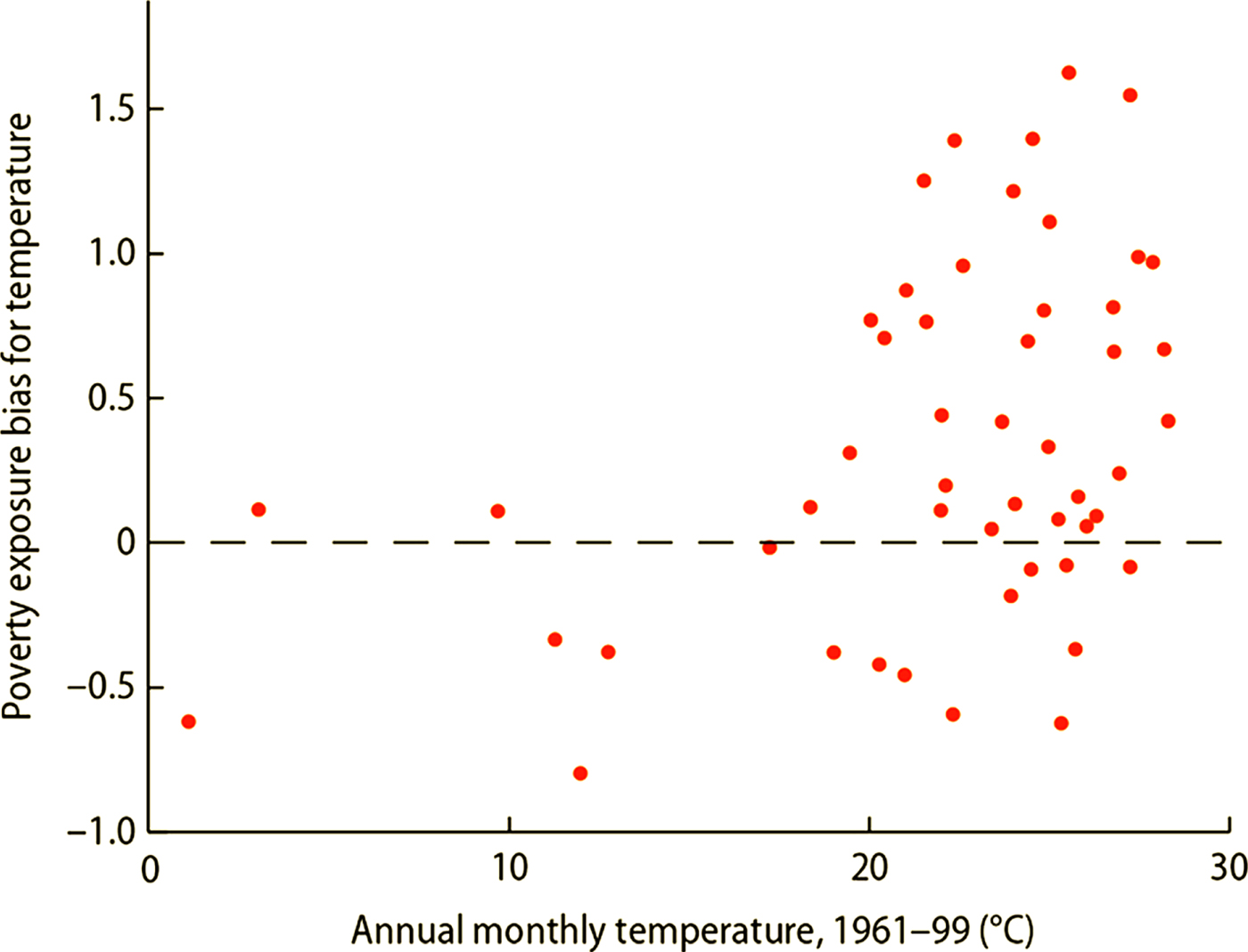
Figure 2. Poor people in hotter countries live in hotter areas, but less so in cooler countries. Note: The poverty exposure bias (y-axis) uses the preferred temperature measure, which examines the number of months each household experiences a monthly temperature above the 98^th percentile. The x-axis provides the annual average of monthly temperature estimates over a 30 year period, to give an indication of each country's climate.

To investigate these results further, we run OLS regressions, examining whether the main PEB (using the relative definition) can be explained by temperature, GDP per capita, share of agriculture, share of population living in urban areas, and a regional dummy, as shown in equation (1):

(1)$$\hbox{PEB}_i =\alpha +B_1 T_i +B_2 \hbox{GDP}_i +B_{3i} Ag_i +B_4 U_i +B_5 \hbox{Reg}_i + \epsilon_i,$$

where PEB is the poverty exposure bias for temperature for country i, T represents the annual average temperature from 1961–99, GDP represents GDP per capita in purchasing power parity, Ag represents the share of employment in agriculture, U represents urbanization rate, and Reg is a regional dummy. For GDP, agriculture share, and urbanization share, the latest data values are used. Data is obtained from the World Bank's World Development Indicators (World Bank, 2017).

Our results are presented in table 2. We find that the only variables that are significantly associated with the PEB are temperature and the regional dummy for Africa.Footnote ⁶ The GDP, agriculture share, and urbanization share have coefficients close to zero and do not approach statistical significance. These results suggest that the PEB phenomenon is not entirely related to GDP or structural transformation – but appears to be related to geography to a larger extent. Future research using time-series and micro-level data (and also examining maximum temperatures instead of averages) might be able to uncover more insights regarding the factors associated with distributional exposure to heat stress.

In summary, these descriptive analyses suggest that the sorting of poor and non-poor households within a country is non-random, but is based at least in part on sub-national trends in temperature within a country.

Table 2. Regression between PEB, GDP, agriculture, urbanization, and region dummy

Notes: Standard errors in parentheses. ***p < 0.01, **p < 0.05

4.1 Country-specific estimates

We investigate the suggestive relationship noted above using simple OLS regressions of the following form:

(2)$$W_{ijt} =\beta_1 \overline {T_{ijt}} +\epsilon_{ijt}.$$

In equation (2), W _ijt represents the wealth percentile of household i in country j surveyed in year t and T _ijt represents average temperature for the hottest month of household i over the period 1960-t, where t is the year of the survey. β₁ is the coefficient of interest, and describes the unconditional relationship between a household's within-country wealth percentile and the average temperature in the vicinity of that household. We also cluster standard errors at the household cluster level to account for potential interactions among households in the same cluster.

Running equation (2) separately for each of the 52 country sub-samples yields a pattern that is consistent with the idea of an optimal temperature zone (full results can be found in appendix C, table A1). Out of the 52 countries surveyed, 23 exhibit a significant negative relationship between temperature and household wealth, 10 exhibit a statistically insignificant relationship, and 19 show a significant positive relationship.

The vast majority of those countries exhibiting negative relationships are tropical countries with hot average climates such as Ghana, Zimbabwe or the Arab Republic of Egypt. For the majority of countries in our data set with average annual temperatures above 20°C, β _1hot < 0 (significant at p < 0.01), which suggests that poorer households tend to be located in hotter, more marginal climates. A similar result is obtained if we use average hottest month temperature to categorize countries by ‘climate’.

To focus on the impact of very extreme heat arising from global warming, it may be desirable to isolate the subsample of unambiguously hot countries, for which relatively high temperatures within the country will almost certainly be associated with greater heat exposure, as opposed to possibly being correlated with reduced cold exposure. Looking at the 21 hottest countries in our sample with average temperatures above 25°C, we note that 14 have significant negative relationships. As a matter of comparison, the United States has an average annual temperature of about 11°C, and an average hottest monthly temperature of 21°C. The fact that some notable hot and poor countries like Indonesia feature positive relationships between household wealth and heat exposure, however, suggests that there might be important dimensions of heterogeneity across omitted characteristics, calling for further investigation.

For the majority of cold countries in the data set – countries with average annual temperatures below 20°C, or coldest monthly average temperatures below 15°C – the opposite is true. That is, β _1cold > 0 for 9 of the 12 countries in our data set with average annual temperatures below 20°C. For cold countries with average annual average temperatures below 15°C, 5 out of 6 feature β _1cold > 0.

This might suggest that, in cold countries, wealthier households self-select into warmer regions due to a higher WTP for milder climates, or that households in more marginal (colder) regions have lower wealth due to greater cold stress. It could also be a function of other omitted correlates such as the quality of institutions or the quality of land. Regardless of the mechanisms, they are consistent with further increases in temperature due to climate change resulting in larger potential welfare impacts for poorer households, due to the way in which the same mean-shift in average temperature leads to a greater increase in hot days for already hot regions, and/or given diminishing marginal utility of consumption.

The magnitudes of β ₁ vary considerably across countries and climates, but are in some cases very large and in general are consistent with previous work documenting across- and within-country gradients in income by temperature. For countries with average temperatures below 15°C, the average significant regression coefficient is 2.4 percentiles per °C. For countries with average temperatures above 20°C, the average significant regression coefficient is −1.3 percentiles per °C. For extremely hot countries – those with average temperatures above 25°C – the average significant regression coefficient is approximately −1.9 percentiles per °C.

The results presented are an unconditional correlation between temperature and wealth, and we find: (1) a strong negative correlation between household wealth and warmer temperature in hot countries, and (2) a strong positive correlation between household wealth and warmer temperatures in cold countries. Higher exposure to heat of poor people can be directly due to temperature-related mechanisms (in either direction, from heat to poverty or from poverty to heat) or due to correlations with other variables (e.g., linked to precipitation, elevation or socio-economic characteristics). As a supplementary analysis, we also present the inclusion of controls, which add value by exploring whether the relationship between poverty and temperature is direct or indirect (e.g., captured through other variables).

To further investigate the conditional links between temperature and wealth, we also run the following specification:

(3)$$W_{ijt} =\beta_1 \overline {T_{ijt}} +X_{ijt} \beta_2 +\epsilon_{ijt}.$$

In equation (3), W _ijt again represents the wealth percentile of household i in country j surveyed in year t; and T _ijt represents average temperature for the hottest month of household i over the period 1960-t, where t is the year of the survey, and X _ijt is a vector of controls: namely, rural/urban status, household size (number of individuals), average annual precipitation, and elevation. We again cluster standard errors at the household level.

The motivation behind including these controls is twofold. Correcting for household size and rural/urban status allows for an interpretation of the wealth index that is closer to a normalized, per capita metric. Correcting for precipitation and elevation allows us to focus on temperature specifically, since there is evidence to suggest that precipitation and elevation both affect residential sorting, and since there is less uncertainty in climate projections regarding temperature increases compared to changes in precipitation patterns.

These conditional results are presented in appendix C, table A2, and the findings are very similar to our unconditional specification for the vast majority of countries (see appendix C, figure A1 for a comparison), supporting the result found above suggesting the importance of temperature. Note that in this case, when including controls, we still cannot conclude about causality: we do not know if people self-sort or if temperature leads to poverty (it is likely that causality runs both ways). Nevertheless, when including controls, we find the existence of a direct relationship between temperature and wealth, with unclear causality.

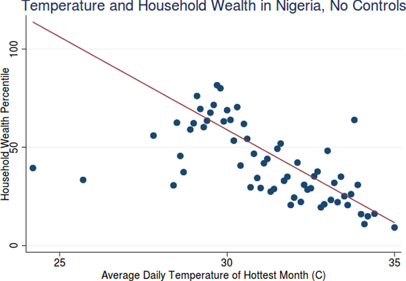
4.2 Country case study: Nigeria (hot)

Taking Nigeria as a representative case study (and using our preferred specification of no controls), we see a strong negative relationship between heat stress and household wealth in the scatterplot in figure 3 (with data points binned by percentile of the temperature distribution). In other words, what this scatterplot does is to divide households into different bins across the temperature distribution, and plots one point for the average of household wealth scores in each bin.Footnote ⁷

Figure 3. Average hottest month temperature and household wealth by temperature bin for Nigeria.

Among the 38,144 households surveyed, households located in places that are exposed to greater degrees of heat stress within the country have systematically lower levels of aggregate wealth. Households located in a grid cell with 1°Celsius warmer hottest temperature tend to be 9.4 percentiles poorer on average. Nigeria is a hot country with an average temperature of 27.3°C (81.2°F) and, as such, one would expect that future climate change would increase heat stress for most if not all households, since most households already reside in areas that are subject to more heat stress than cold stress.

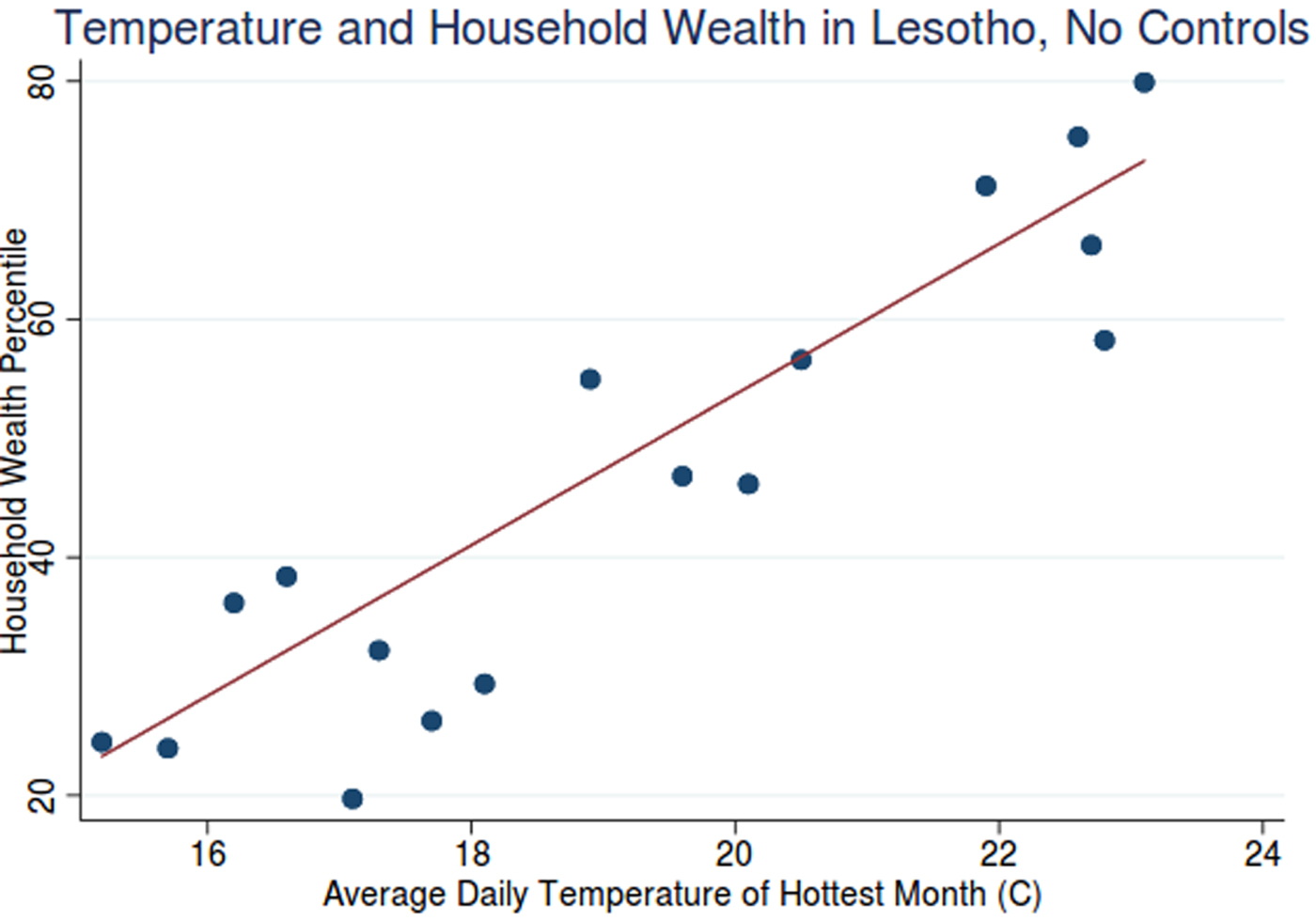
4.3 Country case study: Lesotho (cold)

Lesotho illustrates the opposite effect: a positive relationship between temperature and wealth. Among the 9,226 households surveyed, a 1°Celsius warmer hottest month temperature is associated with a 6.3 percentile higher household wealth score (figure 4). Lesotho is a relatively cold country, with average annual temperatures in the low teens (14.4°Celsius, or roughly 60°Fahrenheit), with winter month temperatures dropping well below freezing. Thus one would expect the relatively warmer households to be closer to the human thermoregulatory optimum, and as such, to suffer fewer cold-related diminutions to labor supply and labor productivity.

Figure 4. Average hottest month temperature and household wealth by temperature bin for Lesotho.

5. Occupational exposure bias

Poorer households may be more likely to engage in work that is more exposed to the elements, in which case we would expect even uniform warming to result in outsized welfare losses for poorer households due to the higher likelihood of heat-related health and productivity impacts. Conversely, it may be the case in some countries that relatively affluent households are employed in sectors more susceptible to heat exposure. This may be true if, for instance, certain skilled trades such as masonry or electrical engineering involve extensive outdoor work in hot climates.

Exposed sectors may include outdoor work-intensive sectors such as agriculture or construction, as well as transportation (e.g. rickshaw drivers) and manual labor intensive industries where air conditioning is missing or inadequate. Understanding the covariance structure between household wealth and occupational exposure to temperature stress is thus an important but as yet unstudied factor that may determine the distributional impacts of heat stress arising from climate change.

We estimate the exposure bias of poorer households arising from occupational choice by constructing an indicator variable denoting whether or not a household has at least one member engaged in an ‘exposed occupation’. We define ‘exposed occupation’ to include agriculture, unskilled manual labor, and military occupations. We also run a specification in which the ‘exposed occupation’ variable does not include agricultural occupations, in order to assess the sensitivity of the results to agriculture.

We fit a logistical regression for the subset of countries (described above) which contains information on household occupations:

$$\hbox{Prob}(I_{ij} =1)={\Phi}(\gamma_{0j} +\gamma_{1j} Y_{ij} +\epsilon_{ij} )$$

where Prob(I _ij = 1) denotes the probability that the indicator variable for exposed occupation is equal to one, and Φ(… is the cumulative standard logistic distribution function. Y _ij denotes the wealth percentile of household i in country j and ϵ_ij denotes a household-, country-specific error term, and we cluster standard errors at the household cluster level. In all the regressions presented, we conduct one analysis per country, since our focus is on examining relationships within countries, leaving comparisons across countries for future research (e.g., using metrics such as the International Wealth Index).

5.1 Household wealth and occupational exposure

We find a clear negative relationship between exposure likelihood and household wealth within all 47 countries for which occupational data are available. In a simple logit unconditional regression of an exposure dummy on household wealth percentile, all resulting coefficients are negative and significant at p < 0.01 (appendix E, table A3). This is driven primarily by the prevalence of agricultural occupations in poorer households. Agricultural occupations account for the vast majority of highly exposed occupations, comprising approximately 38.2 per cent of total respondents’ occupations in the 47 countries for which occupational data are available.Footnote ⁸ As shown in appendix E, table A4, there is no clear relationship between the likelihood of occupational exposure and temperature stress; that is, no clear evidence suggesting that households in hotter climates are more or less likely to work in occupations with greater exposure to the elements.

Nigeria illustrates the typical relationship between household wealth and occupational exposure for a developing country. With a per capita income of roughly US$3,203 (2014) in market exchange rate, Nigeria is a lower middle-income country, with the majority of households engaged in agriculture or manual labor (>51 per cent). Even within Nigeria, it is the poorest households that are more likely to be engaged in manual work that occurs primarily outdoors. Households in Nigeria exhibit a negative relationship between household wealth and occupational temperature exposure, with a logistical regression coefficient of −0.04, significant at the 99 per cent confidence level. This yields the following regression equation:

$$E_{{\rm Nigeria}} = {1 \over \hbox{e}^{0.04138Y_{i,{\rm Nigeria}} -1.597}+1}$$

where E represents the probability of occupational exposure from 0 to 1, and Y _{i, Nigeria} represents household wealth in percentile units. Thus, a household in the 40^th percentile of the wealth distribution has a 48.5 per cent chance of being occupationally exposed, whereas a household in the 60^th percentile has a 29.2 per cent chance (figure 5).

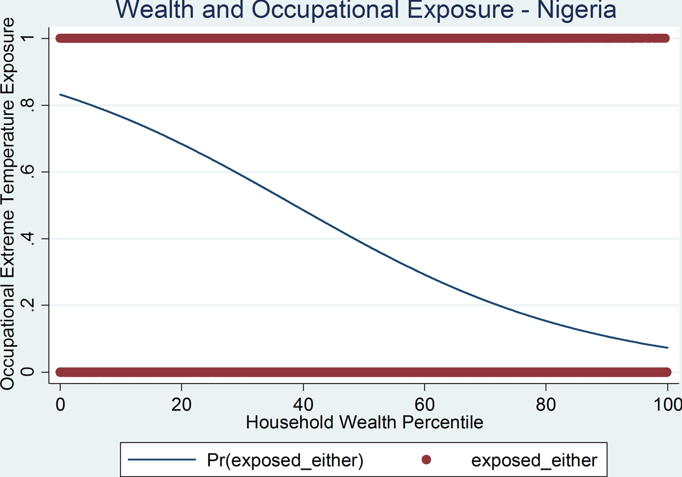
Figure 5. Occupational extreme temperature exposure and household wealth in Nigeria, values fitted by logistical regression. Dummy is 1 if either parent is exposed, 0 if neither is exposed.