


1. Introduction
In this paper we present a study of behavior in a dynamic game with a public bad. Applications of such a setting include the impending social dilemma-type problems like pollution, climate change, depletion of resources and extinction of species, which society is starting to recognize as vitally important. Understanding the behavior of agents in these situations, both with and without regulatory institutions, is useful for policy decisions as many of the relevant regional and global institutions are now being designed and implemented. Global efforts for the past 15 years produced the Kyoto protocol, and examples of regional policies include water buy-back in Australia and biodiversity pilots in the UK. The behavior in environments with dynamic public bads is also of interest from a fundamental research perspective, as such environments represent a relatively novel class of complex dynamic games where human behavior has not been explored in detail.Footnote 1 Experimental studies of behavior in these settings constitute a natural complementary approach to the existing theoreticalFootnote 2 and empiricalFootnote 3 work.
The majority of previous experimental work analyzed strategic interactions in static or repeated game environments. There are a small number of recent studies that focus on non-stationary dynamic problems in the context of public goods (e.g., Battaglini et al., Reference Battaglini, Nunnari and Palfrey2010), pollution and climate change (Saijo et al., Reference Saijo, Sherstyuk, Tarui and Ravago2009), individual management of a renewable resource (Hey et al., Reference Hey, Neugebauer and Sadrieh2009) and common pool resources (e.g., Chermak and Krause, Reference Chermak and Krause2002; Fischer et al., Reference Fischer, Irlenbusch and Sadrieh2004; Ostrom, Reference Ostrom2006; Giordana and Willinger, Reference Giordana and Willinger2007). These games are dynamic in the sense that players make decisions in multiple time periods and the decision problem they face in each period is, in most cases, different due to prior decisions.
We study a dynamic game where subjects in each period decide how much of their endowment to use as a production input. Production generates private revenue and emissions, with the latter contributing to the overall level of pollution that acts as a public bad and imposes a cost on each participant. Unlike in repeated public good games, pollution accumulates over time (with partial dissipation). A similar setting, albeit with some differences in implementation and the main focus, is used by Saijo et al., (Reference Saijo, Sherstyuk, Tarui and Ravago2009), who look at intergenerational transfers of information and utility. In the present paper, we investigate the behavior in a dynamic game with a public bad in an environment with a relatively large number of periods and focus on two main issues: the effects of environmental context and termination uncertainty. Both questions have recently received attention in relation to repeated games.
It was known for a long time in psychology (see, e.g., Goldstein and Weber, Reference Goldstein and Weber1995) and more recently found in a number of experimental studies in economics that behavior in settings with meaningful labeling and context can be different from behavior in otherwise equivalent abstract settings. Two main effects of context have been identified. First, context helps subjects understand complex environments better. For example, Cooper and Kagel, (Reference Cooper and Kagel2003) explore the role of meaningful context in a repeated limit pricing entry game and find that the frequency of strategic play in the presence of context is higher than without it, at least in the initial rounds. In later rounds, the difference declines, indicating that context is a partial substitute for experience. The authors also find some evidence that the reasoning of subjects in the presence of context might be different. Cooper and Kagel, (Reference Cooper and Kagel2009) find that the presence of context facilitates cross-game learning, at least in some situations. Similarly, Chou et al., (Reference Chou, McConnell, Nagel and Plott2009) suggest that context may help game form recognition.
The second possible effect of context is that subjects may invoke preferences related to their experiences outside the laboratory that are not related in any material way to the game being played. For example, Andreoni, (Reference Andreoni1995) finds that the framing of contributions in a linear public good game as positive or negative externalities leads to differences in behavior, with the positive framing generating more cooperation and less free-riding. Messer et al., (Reference Messer, Zarghamee, Kaiser and Schulze2007) find that cooperation in a public good game can be sustained by changing the status quo to full contributions, as opposed to zero contributions, to the public good. In contrast, Abbink and Hennig-Schmidt, (Reference Abbink and Hennig-Schmidt2006) do not identify a significant effect of meaningful context in their bribery game experiment.Footnote 4
In our setting, we are interested in measuring to what extent environmental context promotes pro-environmental behavior and cooperation. One of the reasons meaningful context is rarely used in laboratory economics experiments is the desire of experimenters for more control over preferences and incentives.Footnote 5 The presence of context may invoke subjects' preferences and experiences from outside the lab and thus create additional unobserved heterogeneity that may be correlated with decisions. As pointed out by Cooper and Kagel, (Reference Cooper and Kagel2003), however, the behavior of subjects in experiments with context is of interest as it allows us to better relate the experimental results to behavior outside the lab.Footnote 6 The effect of environmental context has additional implications. If decisions in a treatment with context shift towards lower emission levels, this would indicate that subjects manifest their pro-environmental preferences in the lab. There is evidence that some consumers are willing to pay more for green products (see, e.g., Laroche et al., Reference Laroche, Bergeron and Barbaro-Forleo2001). While pro-environmental decisions have direct impact in the field, observing similar choices in the lab would indicate a stronger pro-environmental preference since there is no actual damage to the environment from laboratory decisions to pollute.
The second design feature we explore is the effect of termination uncertainty. Many real-world dynamic interactions occur under the ‘shadow of the future’ and there may be important differences in behavior in situations with certain and uncertain end.Footnote 7 Games with dynamic externalities are complex, even in the most stylized form, and their complexity is arguably one of the reasons why some of the pro-environmental policies fail. Uncertain termination is an important feature of the environment that adds even more complexity as compared to a finite game, and the comparison between fixed and uncertain termination informs us on how subjects deal with this additional complexity. Termination uncertainty may also reflect decision-makers' discounting of future payoffs, or uncertainty about their own life span.
Our setting is complementary to that of Saijo et al., (Reference Saijo, Sherstyuk, Tarui and Ravago2009) who explored games with dynamic externalities in which subjects do not experience the negative effect of the externality themselves but pass it on to future generations. While the time scale of some elements of climate change indeed spans multiple generations, local public bads – such as pollution from natural gas and oil drilling, fresh water depletion by irrigation systems, or extinction of species – can build up much faster.
Our study is the first to investigate the effect of context and the shadow of the future in a game of a unidirectional dynamic nature. Environmental context reflects one of the key applications of games with a dynamic public bad. While in repeated games subjects face the same decision problem in each period and learning occurs locally – from one period to the next – in our setting subjects face a different decision problem in each period; moreover, the state of the game is determined dynamically by their prior decisions. In the treatment with context we refer to the public bad as ‘pollution’. We also study the effect of experience by letting subjects play the dynamic game twice, starting the second sequence ‘from scratch’. This allows us to observe, in addition to any local learning, global learning across two realizations of the entire dynamic game.
We find that in a fixed-end setting, meaningful environmental context has a strong impact on behavior. Subjects choose lower production inputs, generate less pollution and receive higher payoffs as compared to the no-context case. The effect of context here is different from both Cooper and Kagel, (Reference Cooper and Kagel2003) and Abbink and Hennig-Schmidt, (Reference Abbink and Hennig-Schmidt2006). Being more strategic and playing Nash equilibrium (NE), as predicted by Cooper and Kagel, (Reference Cooper and Kagel2003), would imply producing and, therefore, polluting more, which we do not observe. At the same time, unlike Abbink and Hennig-Schmidt, (Reference Abbink and Hennig-Schmidt2006) who report no effect in their ‘loaded context’ treatment, we do observe the effect of an environmental context. With experience, the difference between the context and context-free treatments reduces substantially. Still, even in the last rounds of the game with fixed end where both the NE and social optimum (SO) solution concepts predict a full scale of production, some subjects in the treatment with context do not produce (and therefore pollute) to the full capacity. We therefore conclude that context substitutes for experience only partially.
Comparing the fixed-end and uncertain-end settings without context, we find no significant difference in behavior for most rounds, with the exception of the few last rounds in the fixed-end (FE) treatment. The effect of experience, however, is different in the two cases. While in the case of uncertain end experience plays practically no role, and the production and pollution levels do not change, in the treatment with fixed end experience has a strong positive effect, reducing own production and improving cooperation. One explanation of this finding may be that in the game with fixed end it is relatively easy to project what the accumulated levels of pollution are going to be since there is no uncertainty about the number of rounds. The experience of negative effect of accumulated pollution can be directly factored into such projection. In contrast, in the game with uncertain end every period has a small but positive probability of being the last one, and subjects may rely less on experience.
The rest of the paper is organized as follows. In section 2, we present the theoretical model and formulate its benchmark predictions. Section 3 describes the experimental design and procedures. The experimental results are reported in section 4. Section 5 contains a discussion and concluding remarks.
2. The model
In this section, we present a model for the dynamic game with a public bad that we use in the experiment. This model is a simplified version of a number of theoretical models of dynamic climate change.Footnote 8
There are n identical risk-neutral players indexed by i. In period t player i has endowment m of a consumption good that can either be consumed directly or used as a production input. Let x it ∈ [0,m] denote the production input chosen by player i in period t (then, (m − x it ) is the part of the endowment consumed directly). The production technology has constant returns to scale, so that input x it is transformed into output Ax it , A > 0. Output is sold in a competitive market at price p (in the units of the consumption good). Let a = Ap denote the resulting rate of return per unit of production input. We will assume that a > 1, i.e., absent any additional considerations, production is more efficient than direct consumption of the endowment.
Production generates emissions proportional to the level of output.Footnote 9 As a normalization, without loss of generality, assume that the amount of emissions generated in period t by processing input x it is equal to x it . The emissions of all players are added to the common pollution level, Y t , which evolves as follows:
 $$Y_{t} = \gamma Y_{t-1}+\sum_{j=1}^{n}x_{jt}\semicolon \; \quad Y_{0} = 0.$$
Here, γ ∈ [0, 1] is the persistence (retention rate) parameter for pollution, which determines the proportion of pollution stock transferred from one period to the next. Parameter (1 − γ), thus, measures the regeneration rate of the environment, or the proportion of pollution stock that gets naturally ‘cleaned up’ within one time period.
Player i's payoff in period t consists of her direct consumption and consumption after production, less the cost of pollution:
 $$\pi_{it} = m - x_{it} + ax_{it} - b\gamma Y_{t-1}.$$
Here b > 0 is the constant unit cost of pollution. Note that the cost of pollution is borne at the beginning of a given period.
We emphasize that, even though the dynamic climate change game bears some mathematical similarity to the standard linear VCM (with the private and public accounts interchanged), there is one crucial difference. The game is inherently dynamic in that the amount of the public bad is transferred from one period to the next and can accumulate over time. Thus, decisions in any given period affect the entire stream of future payoffs.
2.1. Fixed end
Suppose the game described above lasts for T ≥ 1 periods, and T is common knowledge. For theoretical predictions, we use two benchmark solution concepts: subgame-perfect Nash equilibrium (SPNE), and utilitarian SO. The latter is defined as the profile of production inputs that maximizes the sum of payoffs of all players. The results are summarized by the following two propositions. All proofs are given in section B of the online Appendix available at http://journals.cambridge.org/EDE.
Proposition 1
The symmetric SPNE of the T -period game is the profile of production inputs {xt*}, t = 1, …, T, such that xt* = 0 for t < tc N and xt* = m for t ≥ tc N, with tc N specified as follows:
-
(i) if a ≥ 1 + bγ/(1 − γ), then tc N = 1;
-
(ii) if a < 1 + bγ/(1 − γ), then tc N is the smallest positive integer greater than or equal to t N, where
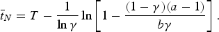
(2) $$\bar{t}_{N} = T - \displaystyle{1 \over \ln \gamma}\ln \left[1- \displaystyle{\lpar 1 - \gamma\rpar \lpar a-1\rpar \over b\gamma}\right].$$
Proposition 2
The symmetric SO of the T-period game is the profile of production inputs {xt S}, t = 1, …, T, such that xt S = 0 for t < tc S and xt S = m for t ≥ tc S, with t ≥ tc S specified as follows:
-
(i) if a ≥ 1 + nbγ/(1 − γ), then tc S = 1;
-
(ii) if a < 1 + nbγ/(1 − γ), then tc S is the smallest positive integer greater than or equal to t S, where
(3)
$$\bar{t}_{S} = T - \displaystyle{1 \over \ln \gamma}\ln \left[1 - \displaystyle{\lpar 1-\gamma\rpar \lpar a-1\rpar \over nb\gamma}\right].$$

Comparing Propositions 1 and 2, we find that in the game with fixed end both the equilibrium and socially optimal profiles of production inputs have the switching structure. In both cases, players allocate nothing to production for some number of periods at the beginning of the game, but at some point switch to allocating everything to production and continue doing so until the end. From equations (2) and (3) it is clear that t c N ≤ t c S. Due to the fact that under the socially optimal scenario each player's payoff reaches a unique maximum, we conclude that the total payoff of the society is strictly greater under the SO scenario than under the SPNE scenario whenever t c N < t c S .
2.2. Uncertain end
Suppose that, instead of a finite time horizon T, in each period there is a continuation probability β ∈ (0, 1) that there will be a next period. Correspondingly, (1 − β) is the termination probability. In this setting, we use Markov perfect Nash equilibrium (MPNE) and SO as the benchmark solution concepts. The MPNE is defined as an equilibrium in Markov strategies, i.e., such strategies that a player's decision in period t is independent of other players' decisions in prior periods.Footnote 10 The SO is defined here as the profile of production inputs that maximizes the sum of total expected payoffs of all players. The results are summarized by the following two propositions.
Proposition 3
The symmetric MPNE in the game with uncertain end is the profile of production inputs {x*t} such that
-
(i) if a ≥ 1 + bβ γ/(1 − β γ), then xt* = m for all t;
-
(ii) if a < 1 + bβ γ/(1 − β γ), then xt* = 0 for all t.
Proposition 4
The symmetric SO in the game with uncertain end is the profile of production inputs {xS t} such that
-
(i) if a ≥ 1 + nbβ γ/(1 − β γ), then xt S = m for all t;
-
(ii) if a < 1 + nbβ γ/(1 − β γ), then xt S = 0 for all t.
With uncertain end, as expected, the MPNE and SO production input profiles are stationary. Due to the fact that the socially optimal profiles of inputs yield a unique maximum to the payoff of the society, the payoff under MPNE is strictly lower than under SO whenever the two production input profiles are different. We conclude that the payoff to the society is strictly lower in the MPNE than in the SO provided that 1 + bβ γ/(1 − β γ)≤ a < 1 + nbβ γ/(1 − β γ).
3. Experimental design and procedures
3.1. Experimental design and research questions
We design three treatments that allow us to measure the effects of environmental context and uncertain termination. In all treatments n = 2, m = 10, a = 5, b = 1, γ = 0.75. The two-person group size allows us to have many independent observations per treatment and simplify coordination.
There are two FE treatments with T = 20. One is the benchmark FE treatment with neutral instructions (FE-N), while the other has instructions with environmental context (FE-C), but is otherwise equivalent to FE-N. For our parameters a > 1 + bγ/(1 − γ) = 4 so, according to Proposition 1, the SPNE profile of production inputs is x t * = 10 for all t = 1, …, 20. At the same time, a < 1 + bγ n/(1 − γ) = 7. The switching point for the SO outcome is t S = 20 − ln (1/3)/ln 0.75 ≈ 16.12, therefore, according to Proposition 2, the socially optimal profile of production inputs is x t S = 0 for t = 1, …, 16 and x t S = 10 for t = 17, …, 20. Thus, both the NE and SO predict inputs equal to 10 in the last few periods, while in the earlier periods the SO and NE solution concepts lead to alternative ‘corner’ predictions.
In the treatment with uncertain end (UE), we use the same parameter values as in the FE treatments, with the exception of the number of periods, which is here uncertain with the continuation probability β = 0.95. Similar to Dal Bó, (Reference Dal Bó2005), we chose the continuation probability so that the expected number of periods in treatment UE is the same as the number of periods in the FE treatments. In the experiment, a random number between 1 and 20 was drawn after each round and shown to subjects. Subjects were informed that if any number between 2 and 20 comes up, there will be a next round, while if number 1 comes up the experiment stops. Four random sequences were pre-drawn and used in our sessions. The minimal number of time periods in the four sequences was 18, so for consistency in treatment UE we cut our data at t = 18 and use the first 18 rounds of data for analysis.Footnote 11
For our parameter values a > 1 + bβ γ/(1 − β γ)≈ 3.48, and, according to Proposition 3, the MPNE profile of production inputs is x t * = 10 for all t ≥ 1. At the same time, a < 1 + nbβ γ/(1 − β γ)≈ 5.96, therefore, according to Proposition 4, the socially optimal profile of production inputs is x t S = 0 for all t ≥ 1. Unlike in the treatments with T = 20, here the two solution concepts lead to stationary predictions on the opposite boundaries.
The dynamic nature of the game implies that decisions in earlier rounds affect the environment in the later rounds; therefore, to test for the effect of experience, each session consisted of two separate decision sequences. Subjects started the first sequence of decisions in the environment described above. Upon termination (either random or deterministic) of the sequence, subjects were informed that they would participate in another sequence in an identical environment while remaining in the same group. For the second part, subjects were restarted with the first round parameters (zero pollution) and their earnings from the second part were added to their earnings from the first part.Footnote 12
The experimental design as well as NE and SO predictions for input levels in each treatment are summarized in table 1. We investigate three key variables: production inputs, x it , and the resulting pollution, Y t , and cumulative payoffs, Π it . Figure 1 illustrates the NE and SO predictions for the dynamics of each of these variables.

Figure 1. Nash equilibrium (NE) and socially optimal (SO) predictions for production inputs (left), pollution (center) and payoffs (right), by period for each treatment
Table 1. Experimental design and theoretical predictions for production inputs, by treatment.

Our first research question addresses the correspondence of behavior with theoretical predictions.
Question 1. To what extent is the observed behavior described by the two benchmark solution concepts, NE and SO?
The second set of research questions addresses the effect of environmental context on decisions. The effect of context may be non-existent since pro-environmental decisions in the lab do not have any actual environmental impact. This finding would be similar to the results of Abbink and Hennig-Schmidt, (Reference Abbink and Hennig-Schmidt2006), who found no effect of loaded instructions on behavior in the bribery game. However, other studies suggest that meaningful context may enhance learning to play strategically and substitute for experience (Cooper and Kagel, Reference Cooper and Kagel2003, Reference Cooper and Kagel2009). In our setting this may imply a tendency to choose production inputs close to the NE or follow conditional cooperation strategies in the spirit of Kreps et al., (Reference Kreps, Milgrom, Roberts and Wilson1982).Footnote 13 On the other hand, the environmental context and emphasis on communal costs of accumulating pollution can lead to lower production inputs due to the presence of pro-environmental preferences and warm glow (similar to Andreoni, Reference Andreoni1995).
Question 2a. What is the effect of environmental context on behavior?
Question 2b. Does context substitute for experience?
The third set of research questions addresses the role of termination uncertainty. Although it was found that the level of cooperation rises in the presence of termination uncertainty in repeated games (e.g., Dal Bó, Reference Dal Bó2005), it is unclear to what extent the results from repeated social dilemmas can be transferred to a dynamic game setting. For our parameter values, the theoretical predictions for behavior in treatments FE and UE are the same, with the exception of the end-game effect in the SO scenario for the FE treatments. Therefore, if subjects follow the NE, we should observe no difference between the FE and UE treatments. If subjects possess some preferences for social efficiency, we would observe different final rounds decisions.
Question 3a. What is the effect of termination uncertainty on behavior?
Question 3b. Is there a change in the effect of termination uncertainty in the presence of experience?
3.2. Procedures
All sessions took place in the XS/FS laboratory at Florida State University. Decisions were made via computer interface using z-Tree (Fischbacher, Reference Fischbacher2007). Subjects were volunteers from the population of undergraduate students at FSU recruited through the online announcement system ORSEE (Greiner, Reference Greiner, Kremer and Macho2004). Each subject participated in the experiment only once. Subjects were randomly assigned to groups, remained in the same group for the entire sequence of decisions and were unaware of the identities of other group members. Experimental instructions, available in section A of the online Appendix, were read out loud, with a paper copy distributed to subjects to follow. After the instructions, subjects were guided through a sample round of decisions to become familiar with the interface, and then filled out a paper-based questionnaire to make sure they understood how the game works. The experimenters checked each subject's questionnaire individually.Footnote 14 Each session lasted about 90 minutes, with subjects earning about US$ 20 on average, including a US$ 10 show-up fee.
4. Results
We next present and discuss the results of two comparisons between treatments. The first comparison is between treatments FE-N and FE-C and aims at assessing the impact of context on subjects' decisions and outcomes. The goal of the second comparison, between treatments FE-N and UE, is to measure the impact of UE (or the ‘shadow of the future’, Dal Bó, Reference Dal Bó2005). These comparisons are made between subjects. Additionally, in all treatments subjects played the dynamic game twice, which allows us to look at the role of experience in a within-subject manner.
For each comparison, we discuss the impact of treatment and experience on subjects' decisions (production inputs) and outcome variables (pollution levels and payoffs). Figure 2 shows the average per capita production inputs (left), average pollution levels (center), and average per capita cumulative payoffs (right) by period for each of the treatments. Additionally, figure 2 shows the benchmark theoretical predictions (NE and SO) for the corresponding variables.

Figure 2. Left: Mean per capita production inputs, by period. The solid lines show the Nash equilibrium (NE) and socially optimal (SO) levels. The vertical dashed lines represent switching from xit = 0 to xit = 10 in period 17 for the SO profile in the FE treatments. Center: Mean pollution levels, by period. Right: Mean per capita cumulative payoffs, by period. The solid lines show the Nash equilibrium (NE) and socially optimal (SO) levels. The solid lines show the Nash equilibrium (NE) and socially optimal (SO) levels. The theoretical curves are obtained by connecting discrete dots for better visualization
The results of statistical comparisons between treatments are presented in section C of the online Appendix. There, the experimental data for each variable are shown with group-level error bars (figure C1). Also, tables C1, C2, and C3 show the period-by-period differences between the treatments for each variable, with group-level standard errors and significance levels.
4.1. The role of context
In part 1 of the experiment, production inputs are significantly lower in treatment FE-C than in treatment FE-N. This is seen from figure 2 (left), and confirmed by figure C1 and table C1 (online Appendix, section C). There is a pronounced end effect in both treatments, with a sharp increase in average inputs in the last four periods. In period 20, nearly all subjects choose the maximal input in treatment FE-N, while a slightly (but insignificantly) lower average input is chosen in treatment FE-C.
In part 2 of the experiment, although inputs in treatment FE-C remain lower than those in FE-N in all periods, the difference is not statistically significant in most of the periods. There is a strong end-game effect in both treatments, similar to part 1. Interestingly, in the last three periods the FE-C inputs, although high, are significantly lower than the FE-N inputs (the latter reach the maximal level of 10 for all subjects in period 20). We therefore conclude that context partially substitutes for experience. The statistically significant lower production allocation in the last periods indicates that with context some subjects follow with environmentally friendly behavior even at a clear cost. We conjecture that with context subjects may assign some moral value to their decision even in the laboratory.
These patterns of inputs have consequences for pollution levels (figure 2, center) and payoffs (figure 2, right). In both treatments FE-N and FE-C, pollution rises rapidly at the beginning of the game, then somewhat stabilizes, and finally sharply rises again due to the end-game effect. Pollution is substantially lower in the treatment with context in part 1 of the experiment. In part 2, pollution is drastically reduced in the treatment without context (as compared to part 1) and, although it remains higher than in the treatment with context in all periods, is not significantly different between the two treatments (cf. table C2, online Appendix section C).
Payoffs in treatment FE-C are initially lower than in treatment FE-N, but they equalize between periods 12 and 16, and become significantly higher in the later periods of part 1 (cf. figure 2, right, and table C3 in the online Appendix section C). The relatively high production inputs in FE-N allow subjects to earn more initially, until pollution builds up, but ultimately the accumulating costs of pollution become so much higher in FE-N that the payoffs fall short of those in FE-C.
Defining sustainability as the ability to have non-decreasing long-run payoffs, we infer from figure 2 (right) that in part 1 sustainability is reached in treatment FE-C but not in treatment FE-N. In part 2 of the experiment, the payoffs in FE-C are higher in the last rounds; however, there is no significant difference in payoffs between treatments FE-N and FE-C, and in both treatments subjects reach sustainability by the end of the game.
To summarize, the comparison between treatments FE-N and FE-C leads to the following findings.
Finding 1
Without experience, production inputs are lower, pollution levels are lower, and long-run payoffs are higher in FE-C than in FE-N.
Finding 2
With experience, the difference between production inputs without context and with context is not statistically significant. There are no significant differences in the pollution levels and payoffs. There is, however, a systematic difference in the end-game effect, and production inputs in the treatment with context are significantly lower in the final rounds.
Our findings are related to those of Cooper and Kagel (Reference Cooper and Kagel2003, Reference Cooper and Kagel2009) who studied the effect of a meaningful context on strategic behavior in signaling games and found that context partially substitutes for experience. In our setting, context moves subjects in the direction of cooperation, i.e., away from the strategic behavior predicted by the SPNE. At the same time, the observed behavior in the context treatment follows more closely the pattern of conditional cooperation in finitely repeated prisoner's dilemma games (e.g., Kreps et al., Reference Kreps, Milgrom, Roberts and Wilson1982) and is more efficient.
In order to specifically test whether context substitutes for experience, we performed the period-by-period comparison of average inputs in part 1 of treatment FE-C and in part 2 of treatment FE-N. With the exception of five periods (periods 15–19), the difference is not statistically significant, although it always has the same sign. Thus, experience and context partially substitute for each other, with a significant difference only in the end-game effects.
Finding 3
Experience substitutes for context, with the exception of the final few rounds of decisions.
The difference in the end-game effect between treatments FE-N and FE-C can be explained as follows. Regardless of context, in period 20, even in the presence of conditional cooperation and other-regarding preferences, it is a dominant strategy to contribute m to production, and this is almost unanimously chosen in treatment FE-N. In the presence of context, however, many subjects contribute less than m until the end, even in period 20, which leads to the observed significant difference between treatments in the final periods. The difference suggests that in the presence of context, subjects are more averse to making a decision to pollute even when contributing to the public bad has no effect on payoffs. This is consistent with the general effect of context encouraging pro-environmental behavior despite the fact that such behavior in a laboratory game has no effect on the actual pollution.
4.2. Fixed versus uncertain end
Comparing treatments FE-N and UE, it is seen from figure 2 (left) and table C1 (online Appendix) that there is no statistically significant difference in average inputs in part 1, with the exception of the end-game effect in treatment FE-N. In part 2, however, inputs in treatment FE-N are significantly lower than in UE until the very last periods.
The results for production inputs have consequences for pollution level and payoffs. In part 1 of treatment UE, pollution grows at a decreasing rate and eventually stabilizes, whereas in part 1 of treatment FE-N there is a pronounced end-game effect with rapid growth. Apart from the last few rounds, the difference in pollution levels between the two treatments is not significant. In part 2, the pollution level becomes lower in treatment FE-N than in UE, and this holds for all except the last few rounds due to the end-game behavior in FE-N. There is no significant effect of experience in treatment UE where the pollution levels in part 2 are not different from those in part 1. At the same time, as expected from the analysis of production inputs, in treatment FE-N pollution decreased significantly in part 2 compared to part 1 (this holds for most rounds with the exception of the end of the game where they become the same).
For payoffs, there is no significant difference between the two treatments in part 1. In both treatments, subjects do not reach sustainability. In part 2, the payoffs in treatment FE-N are significantly higher than in treatment UE. Sustainability is not reached in UE even with experience.
The results can be summarized as follows.
Finding 4
Without experience, inputs in the treatments with FE and UE are not different for most periods with the exception of the end-game effect in the former.
Finding 5
Experience has a strong effect on behavior in the treatment with FE where production inputs become lower, and has practically no effect in the treatment with UE.
We note that Finding 4 is interesting in light of the results of Dal Bó, (Reference Dal Bó2005), who found higher levels of cooperation in repeated prisoner's dilemma games with uncertain end, as compared to games with a fixed number of periods equal to the expected number of periods in the game with uncertain end (as is the case here). Even more striking in this regard is Finding 5: when given a chance to play the same game again, subjects exhibited much higher levels of cooperation in the treatment with certain end than in the one with uncertain end. We conclude that the ‘shadow of the future’ may have the opposite effect in non-stationary games. In our setting it is slowing down the process of learning to cooperate to reduce the public bad. This effect may be due to greater complexity in terms of uncertainty of the last period and that subjects view prior history as less reliable, especially if they are too optimistic about the probability of the game ending sooner.
4.3. Dynamics in subjects' production decisions
In this section, we explore the effect of meaningful context and uncertain end on the dynamics of subjects' individual decisions. Let x it denote the production input of player i in period t, x it other – the production input of the other member of player i's group in period t, and Y it – the pollution level in player i's group at the end of period t. In the treatments with FE we expect strong end-game effects. According to the theoretical predictions for our parameter values, the SO profile of production inputs switches from 0 to m in period 17. We therefore introduce a dummy variable D t ≥ 17 equal to 1 for t ≥ 17 and zero otherwise, to control for the end-game effect. We also use the trend variable, t, to control for non-stationarity in decisions.
The resulting population model is:
 $$x_{it} = \beta_{0} + \rho x_{i\comma t-1} + \beta_{1}x_{i\comma t-1}^{other} + \beta_{2}Y_{i\comma t-1} + \beta_{3}t + \beta_{4}D_{t\geq 17} + u_{it}.$$
Here, ρ and β0 through β4 are the model coefficients; u it is the zero-mean idiosyncratic error term.
We perform estimation of model (4) using OLS with robust standard errors clustered at the individual level. We note that estimation methods explicitly taking into account possible unobserved heterogeneity, such as fixed effects or random effects, are not applicable to model (4) due to the presence of the lagged dependent variable, x i, t−1, and a predetermined variable Y i, t−1 (Wooldridge, Reference Wooldridge2002). The reason is that the strict exogeneity assumption required for fixed and random effects methods to work is violated here. The OLS estimation, on the other hand, only requires the contemporaneous exogeneity assumption, which is less restrictive and can, at least in principle, hold in such models. The unobserved heterogeneity is here captured through the initial condition.Footnote 15
The results of the estimation are presented in table 2. We first discuss the results pertaining to the effect of context under the fixed-end condition (comparing treatments FE-N and FE-C), and then the results regarding the effect of termination uncertainty (comparing treatments FE-N and UE).
Table 2. OLS regression results for model (4), by treatment.

Notes. Cluster-robust standard errors in parentheses. Significance levels: **, 1%, *, 5%, 10%.
Comparing the regression results for treatments FE-N and FE-C in part 1, there are two major differences in dynamics between the two treatments. First, persistence in production inputs is much stronger in treatment FE-C (p = 0.0105 for a two-sided t-test of the equality of coefficients). Second, the end-game effect is stronger in FE-C (p = 0.0824 for a two-sided t-test of the equality of coefficients). The latter effect, however, is a consequence of the average level of inputs for t < 17 being lower in FE-C. The stronger persistence in FE-C implies that in the presence of context subjects' decisions are determined to a greater extent by their intrinsic motivations and preferences. This is to be expected, as context likely invokes stronger individual heterogeneity and attachment to one's own behavioral type. In both treatments, there is a positive reciprocity measured by the coefficient at the other group member's input, x i,t−1 other . This is consistent with inequity aversion in decisions: if one of the players increases her production, the other does so as well, even at a cost of creating more pollution, to equalize payoffs.Footnote 16 The reaction to the total amount of pollution in the previous period, Y i, t−1, albeit not significant in FE-N, is not statistically different between the two treatments. In part 2, the persistence in subjects' decisions increases in FE-N and reaches the same level as in FE-C. This confirms the conjecture that context and experience are substitutes, and also points at the additional heterogeneity and attachment to one's own type that emerges without context after part 1.
Comparing treatments FE-N and UE, the first observation is that, as expected, there are no end-game effects in the treatment with UE. Otherwise, there are no differences in dynamics between the two treatments. Persistence in decisions increases significantly between parts 1 and 2 in both treatments. Thus, at least in terms of persistence, under the uncertain-end condition experience plays a role similar to the one discussed above for treatment FE-N.
In addition to local learning captured by equation (4), we analyzed global learning across the two sequences (part 1 and part 2) of the dynamic game. Subjects stayed matched with the same opponent throughout both parts, which makes the environment the most conductive one for such learning. Global learning could entail learning about the nature of the game as well as learning about the opponent. To see how subjects' behavior in part 2 is related to their experience in part 1, we constructed a scatter plot where each point represents a pair of subjects, with the average production input of the pair in part 1 on the horizontal axis and the average production input of the same pair in part 2 on the vertical axis. The results for each treatment are shown in figure 3. Interestingly, while in treatments without context, FE-N and UE, the patterns are qualitatively similar, with many pairs reducing their emissions in part 2 (more so in FE-N thus leading to lower overall emissions in that treatment), in the treatment with context most pairs choose the same input levels across the two parts. While this result is in part due to the fact that more pairs chose low emission levels already in part 1, this is another illustration of the substitution between context and experience.

Figure 3. Average group input in part 2 vs. average group input in part 1 for each group, by treatment
We summarize our findings as follows.
Finding 6
In the presence of context without experience, the dynamics of decisions has stronger persistence, indicating more heterogeneity and attachment to one's own type. With experience, the difference in persistence between the context and no-context conditions disappears.
Finding 7
There is no effect of termination uncertainty on the dynamics of decisions, with the exception of the end-game effects. In particular, the effect of experience on persistence is similar under the fixed-end and uncertain-end conditions.
Finding 8
In the presence of context, there is little evidence of learning across the two sequences of the dynamic game. Without context, most groups reduce their input levels (and emissions) in part 2.
Experience helps subjects understand the game better and may also serve as a coordination device since subjects remain in the same group and are aware that all group members experienced the same negative consequences of the growing public bad in the previous part. Context can also work as a coordination device on lower initial levels of production and pollution leading to higher persistence without experience, which is consistent with the data.
5. Discussion and conclusions
This paper presents the first experimental study of the effect of environmental context and termination uncertainty in games with a dynamic public bad. Such a setup contributes to the emerging experimental literature on non-stationary dynamic externalities and public goods. The important practical applications include production decisions in an environment with dynamic costs of pollution and climate change. The problem of climate change is recognized as one of the urgent global issues; however, there are just a few experimental studies that look at the behavior in similar environments. The need to better understand decisions of participants in dynamic games with a public bad is evident from the reports of insufficient response to incentives in a number of practically implemented institutions, including the Kyoto protocol.
In this study we investigate the fundamentals of decision making in a dynamic setting with a public bad, and our results serve as a starting ground for further studies of behavior in the presence of regulatory institutions. Our two main treatment variables are the environmental context and termination uncertainty. The motivation for these treatments comes from the field and from the existing experimental literature.
One of the conjectures for slow response to environmental regulation is the argument of fixed lifetime, in the sense that individuals care less about the state of the world where they are no longer living. If that is the case, decision makers view the situation in some way as a fixed-end game and would tend to produce and, therefore, pollute more as the termination point approaches. Although some experimental studies investigated the effect of termination uncertainty in repeated social-dilemma type games (see, e.g., Dal Bó, Reference Dal Bó2005), the implications for dynamic games may differ due to the evolution of the decision problem subjects are facing.
Comparing our experimental results to the theory, we use two benchmark solution concepts – the myopic payoff-maximizing MPNE and the utilitarian SO. In our design, the two solution concepts lead to different predictions for the UE and FE treatments. While the NE for both treatments is full allocation to production, the SO allocation stays at zero in the UE treatment and switches from zero to full allocation for a few last rounds in the fixed-end treatment. The observed production decisions for all except the final few rounds are between the SO and Nash in both treatments. This is not unexpected, as the existing experimental literature on dynamic decision making (e.g., Noussair and Olson, Reference Noussair and Olson1997) suggests that even simple non-stationary dynamic problems are too difficult for most subjects. Moreover, it has been established that most subjects do not backward induct beyond a few rounds in finite dynamic games, especially when doing so is not socially optimal (e.g., Selten and Stoecker, Reference Selten and Stoecker1986; McKelvey and Palfrey, Reference McKelvey and Palfrey1992).
There is no difference in behavior between the FE and UE treatments without experience, with the exception of the strong end-game effect in the FE treatment. In the last few rounds, production inputs remain relatively stable in the UE treatment while there is a clear end-game effect with full allocation to production in the FE treatment. With experience, however, the difference between treatments becomes significant even for early and intermediate rounds. Production allocations in the FE treatment are significantly lower with experience for all except the last few rounds where, as expected, they again converge to maximal production. In contrast, experience has practically no effect in the treatment with UE. There is no effect of termination uncertainty on the dynamics of decisions, with the exception of the end-game effects. In particular, the effect of experience on persistence is similar under the fixed-end and uncertain-end conditions.
Thus, we find that the effect of uncertain termination in non-stationary dynamic games is different from infinitely repeated games (e.g., Dal Bó, Reference Dal Bó2005). Unlike in our setting, Dal Bó, (Reference Dal Bó2005) finds that the presence of termination uncertainty improves cooperation, and his results generally support the comparative statics of the theory of infinitely repeated games based on expected payoff maximization. Our results suggest that dynamic games are more difficult for subjects to understand, and the presence of termination uncertainty creates an additional difficulty. This may explain why after the restart subjects in the FE treatment cooperate much better and reach higher payoffs but in the UE treatment they do not have enough time to grasp the entire dynamic game and do not show any significant adjustment. Of course, the non-stationarity of our setting is not the only difference from the experiments of Dal Bó, (Reference Dal Bó2005). Our game lasted, on average, 20 periods whereas Dal Bó used repeated prisoner's dilemma games of two or four rounds on average. Therefore, in the case of fixed end, subjects were more likely to apply backward induction in his setting, while in our setting subjects could view the FE treatment as a ‘certain continuation game’ until the last few rounds and thus had more incentives to cooperate. Additionally, Dal Bó lets subjects play up to 10 repeated game sequences, while we only have two. These factors may have also contributed to the differences in results.Footnote 17
Environmental context has a significant effect on decisions, with production inputs and pollution levels lower and payoffs higher compared to the neutral context treatment. This effect is consistent with a pro-social rather than own payoff-maximizing NE strategy, which is different from the effect of meaningful context in Cooper and Kagel, (Reference Cooper and Kagel2003). At the same time, the presence of a significant effect is consistent with Cooper and Kagel and different from Abbink and Hennig-Schmidt, (Reference Abbink and Hennig-Schmidt2006). With experience, i.e., after the restart, production decisions as well as pollution remain lower with context although the effect is no longer statistically significant except for the last few rounds. Unlike in the neutral context treatment, in the treatment with environmental context average production inputs remain below the dominant strategy of maximal production in the last few rounds. Environmental context, therefore, partially substitutes for experience, which is similar to the findings of Cooper and Kagel (Reference Cooper and Kagel2003, Reference Cooper and Kagel2009).
The manifestation of environmental preferences in the laboratory also suggests that subjects receive utility from taking a pro-environmental action even if this action has no real impact in the field. When subjects have environmentally friendly preferences they are willing to forgo profits to manifest a pro-environmental action. This finding is in line with the recent results on the effect of ‘green’ advertisement on consumer behavior (see, e.g., Cason and Gangadharan, Reference Cason and Gangadharan2002; Vermier and Verbeke, Reference Vermier and Verbeke2006; Hartmann and Apaolaza-Ibáñez, Reference Hartmann and Apaolaza-Ibáñez2010). Our results on the impact of environmental context contribute to the literature on the effects of framing in economics experiments. In our setting, framing the experiment in environmental terms facilitates understanding of the game and also invokes subjects' environmental preferences. Such preferences, formed naturally outside the lab, assign a ‘moral’ connotation to the public bad, and thus promote cooperation.
Supplementary material and methods
The Supplementary material referred to in this paper can be found online at journals.Cambridge.org/EDE.


