2.1 The forest transition concept

The forest transition concept as introduced by Mather (Reference Mather1992) refers to the switch from decreasing to expanding forest area that has been observed in many developed nations in the past, and recently in several developing countries (Rudel et al., Reference Rudel, Coomes, Moran, Achard, Angelsen, Xu and Lambin2005; Lambin and Meyfroidt, Reference Lambin and Meyfroidt2010). In the transition curve, a long phase of deforestation is followed by a similarly long phase of reforestation. The point where forest cover reaches its minimum is the transition to which we also refer here as the turning point. Figure 1 illustrates the forest transition along with the expected U-shaped path of net forest cover through time.

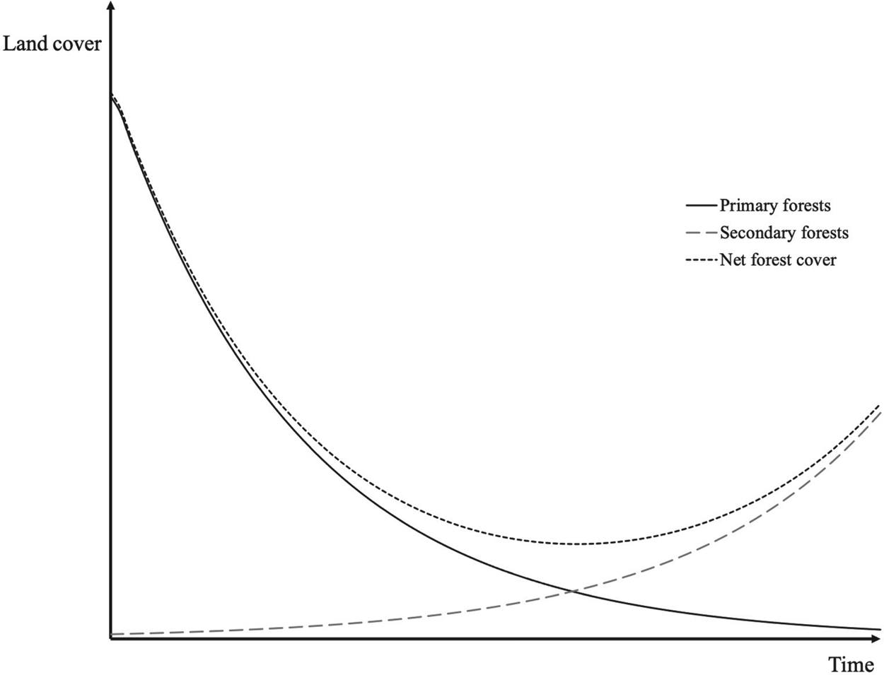
Figure 1. A decomposition of Mather (Reference Mather1992) forest transition.

Prior to Mather's seminal paper, different studies reported that the evolution of the forest cover in a country follows a U-shape form. For instance, Clawson (Reference Clawson1979) studied the US case, finding that forest cover started decreasing at the beginning of the nineteenth century, then stabilized and increased around the mid-1900s. Forest depletion was at its highest level between 1800 and 1900, and decreased at the beginning of the twentieth century. A forest cover increase occurred around 1920, through net timber growth, as a consequence of the previous decline in standing volume. In France, it occurred over a longer time period than in the US, less forest cover was preserved, and the turning point took place during the nineteenth century (Mather et al., Reference Mather, Fairbairn and Needle1999). In India, according to data from Foster and Rosenzweig (Reference Foster and Rosenzweig2003), the turning point occurred around 1960, with forest cover at the time of about 16 per cent of total land. In China, Rudel et al. (Reference Rudel, Coomes, Moran, Achard, Angelsen, Xu and Lambin2005) mention that only 7 per cent of forest cover was left when the turning point occurred a few decades ago.

As suggested by these various cases, the timing and the intensity of forest transitions are particular to each country, and the forest transition approach does not constitute a prediction of what necessarily happens in a country experiencing deforestation. Nevertheless, it allows us to emphasize common features behind the long-term deforestation process in a given country: deforestation, stabilization, reforestation. Yet this concept does not predict the particularities of those dynamics, which are dependent on each country's characteristics. Those particularities encompass the pattern and length of the forest transition curve, the nature of the turning point, and the composition of the land use once the transition ends. For instance, a particular country may end deforestation only when all the primary forests have been converted, or may not experience any reforestation.

Different articles, mostly descriptive, have attempted to describe the economic schemes that lead to a forest transition in a country. Based on observations of developed nations, Rudel et al. (Reference Rudel, Coomes, Moran, Achard, Angelsen, Xu and Lambin2005) explained the occurrence of the turning point using either an economic development or a forest scarcity pathway. The economic development path states that the capital stock formed during agricultural land expansion is reinvested in new, more profitable sectors, which do not require intensive use of forests. Industry-based production increases along with creation of new urban jobs with higher wages that attract farmers from frontiers to urban areas. Some previously cropped lands therefore return to forest. During this period, governments – which may have become more responsive to ecological and climatic problems – may also implement reforestation programs.

The scarcity path argues that the relative scarcity of land held in forests serves to increase timber prices while leading to potentially high environmental damages due to the lack of forest cover. In order to benefit from the high forest rents and control environmental degradation, large-scale plantations are implemented through investments. The net deforestation rate becomes zero or negative, and the turning point occurs. Additionally, globalization can favor the end of deforestation (i.e., a turning point) by trading ecological ideologies, new patterns of demand, or by developing tourism (Kull et al., Reference Kull, Ibrahim and Meredith2007; Lambin and Meyfroidt, Reference Lambin and Meyfroidt2010). Through a study of several developing countries between 1990–2010, Wolfersberger et al. (Reference Wolfersberger, Delacote and Garcia2015) indeed find that institutional quality also promoted the occurrence of this turning point in many cases, as well as evidence of both the forest scarcity and economic development paths.

As noted in the introduction, previous theoretical economic analysis that considers the dynamics of long-term forest conversion is sparse and has focused mainly on the first deforestation phase in figure 1, that is, before the turning point is reached (e.g., Hartwick et al., Reference Hartwick, Van Long and Tian2001; Barbier et al., Reference Barbier, Damania and Léonard2005; Ollivier, Reference Ollivier2012). Other work prior to these studies include Ehui et al. (Reference Ehui, Hertel and Preckel1990), which studied deforestation and agricultural expansion in an economy where cumulative deforestation impacts agricultural yields. The authors notably examined the impact on the deforestation rate of changes in discount rates and marginal returns from agriculture. However, they did not consider different types of forest, tenure costs implications or the application of public policies.

Finally, note that the traditional forest economics literature has developed models that distinguish forest types such as old-growth, natural secondary growth and man-made forests (e.g., Lyon and Sedjo, Reference Lyon and Sedjo1983; Vincent and Binkley, Reference Vincent, Binkley and Sharman1992; Conrad, Reference Conrad1999; Sohngen et al., Reference Sohngen, Mendelsohn and Sedjo1999). However, their work does not consider agricultural land use or aspects of the forest transition which are important in this paper.

2.2 The importance of distinguishing primary and secondary forests

The absence of secondary forests in theoretical economics discussions of long-term deforestation is not consistent with purely empirical studies showing that, during development, primary and secondary forests follow two opposite paths that establish the existence of a turning point. Primary forests tend to decrease while secondary forests increase, but this was not clearly defined in Mather's work. Grainger (Reference Grainger1995) reported this issue regarding Mather's original description of the forest transition, and talked instead about two separate processes. According to Grainger (Reference Grainger1995), the ‘national land use transition’ corresponds to the large depletion of primary forests, while the ‘forest replenishment period’ corresponds to the period of secondary forest plantations and natural regeneration, also explained in Barbier et al. (Reference Barbier, Burgess and Grainger2010) and Barbier et al. (Reference Barbier, Delacote and Wolfersberger2017). What must be understood here is that the two processes refer to two separate forest stocks (primary and secondary), but that they are not completely independent of each other. The forest replenishment period may take place because the national land use transition raised prices of forest products (by the scarcity effect) or, for instance, involved environmental issues (biodiversity losses, soil degradation, etc.).

Further empirical motivations for our work are provided by Mather (Reference Mather2007) and Perz and Skole (Reference Perz and Skole2003) who analyze data from Amazonia and Asia (China, India and Vietnam), respectively, and claim that the forest transition concept requires refinements, notably since they found, on the basis of poor available data at the time, that the net increase of forest cover was largely composed of plantations. Likewise, for public policy purposes, Angelsen and Rudel (Reference Angelsen and Rudel2013) also highlight the importance of going beyond the ‘forest-nonforest dichotomy’ within the forest transition concept. They argue that, because of differences in ecosystem services attributed to carbon storage capabilities, considering only net forest cover as a policy target would lead to protection of low carbon landscapes. This is in line with the work of Kauppi et al. (Reference Kauppi, Ausubel, Fang, Mather, Sedjo and Waggoner2006) on carbon and forest biomass which extends the forest area transition to a forest carbon transition, and also incorporates distinctions between primary and secondary forests in the framework.

The distinction between primary and secondary forests that we include in our model also reflects work in climate ecology. Luyssaert et al. (Reference Luyssaert, Sebastiaan, Schulze, Börner, Knohl, Hessenmoller, Law, Ciais and Grace2008, 213) find that old growth forests can store centuries worth of carbon reserves, and ‘can continue to accumulate carbon, contrary to the long-standing view that they are carbon neutral’. Regarding carbon dioxide emission, it is therefore more efficient at least over the short- and mid-terms to conserve older forests rather than seek to plant new ones. Concerning biodiversity, Burley (Reference Burley2002) finds that tropical forests are home to 50 per cent of the known vertebrates and 60 per cent of plant species. He argues that forests reestablished on current non-forest land as plantations cannot lead to full recovery of all of these species, especially if some agricultural activities took place prior to reforestation. In addition, Gibson et al. (Reference Gibson, Lee, Koh, Brook, Gardner, Barlow, Peres, Bradshaw, Laurance, Lovejoy and Sodhi2011) find that primary forests were irreplaceable in their ability to maintain tropical biodiversity.

The conclusion from this literature establishes that secondary forests indeed have a lower marginal environmental value than primary ones in terms of both carbon storage and biodiversity provision, especially in the short run. It therefore follows that making a distinction between the types of forest (i.e., primary or secondary forests) is necessary since deforestation of primary forests is irreversible, in the sense that replacement by secondary forests leads to imperfect substitutes in terms of the ecosystem services that can be produced from any land unit.

The motivation for our paper thus comes from the following critical observations made in this section: (1) the forest transition concept is a useful tool to understand the long-term dynamics of a country's forest cover; (2) it is important to take into account different types of forests in order to account for known economic and ecological non-substitutability of primary and secondary forests; (3) the theoretical economics literature approaching a forest transition framework only focuses on deforestation and does not consider reforestation, or the primary-versus-secondary-forests dichotomy; and (4) the economics literature focusing on the links between primary and secondary forest focuses more on the forest sector implications (such as timber markets) and does not investigate either the land use implications of the transition, or the differing land tenure security of the various types of forests and agricultural land.

The ambition of our paper is thus to offer a bridge between the land use and forest clearing articles commonly used to study the dynamics of deforestation. Our model is most closely related to that of Hartwick et al. (Reference Hartwick, Van Long and Tian2001), but we additionally integrate the double dynamics of deforestation and reforestation, explicitly taking into account the distinction between primary and secondary forests. Our contribution is, in this context, to investigate how a country's particularities may determine several key components of a forest transition, namely: (i) the length of the forest transition (speed of deforestation and reforestation), (ii) the remaining forest cover at the turning point (net cumulative deforestation), and (iii) the forest composition once the forest transition is achieved (respective importance of primary versus secondary forests).

3.1 The model

Consider a small open economy with a representative land user allocating a land endowment normalized to one unit to primary forests ($F_{t}$), secondary forests ($S_{t}$) and agriculture ($1-F_{t}-S_{t}$). Initial primary and secondary forest cover is given by $F_{0}$ and $S_{0}$, respectively. Because it is the most relevant approach for our research question, throughout the paper we will focus on the study of an economy with high initial primary forest cover $F_{0}$, and low initial agricultural land cover and secondary forest cover $S_{0}$. Agricultural land expansion will thus represent the main driver of forest transition, as empirically observed.

Let $f(F_{t})$ and $g(S_{t})$ be the land rents associated with primary and secondary forests respectively, at any time $t$. By primary forests, we mean forests where human activities imply small if any perturbations, and we assume that $f(.)$ follows the standard properties $f^{\prime }(F_{t})>0$, $f^{\prime \prime }(F_{t})<0$. By secondary forests, we mean forests strongly impacted by human activities, and forests generated by plantations. The function $g(.)$ is also assumed increasing and strictly concave, that is, $g^{\prime }(S_{t})>0$ and $g^{\prime \prime }(S_{t})<0$. Thus, there are three types of forests accommodated in our model: natural old-growth forests, secondary new-growth forests from natural regeneration, and secondary planted forests. In our model, secondary forests encompass both new-growth forests and plantations.Footnote ¹

Primary forest rents include the public good value associated with an old-growth standing forest, such as carbon stock, biodiversity benefits, soil protection or water supply. Secondary forests generate rents that include sustainable timber harvesting and public good values such as flows of sequestered carbon, for instance. The differences in rents can be explained by various characteristics or preferences of the representative land user, depending on the value they attach to timber harvesting and forest environmental services.

Finally, let $h(1-F_{t}-S_{t})$ be the rents obtained from land under agriculture. In light of the fact that rents take into consideration both timber and public good benefits, in our setting $f(F_{t})$, $g(S_{t})$ and $h(1-F_{t}-S_{t})$ reveal the preferences of a representative land user toward different sources of rents. With those three, unspecified, rent functions, our model is flexible enough to describe a wide range of very diverse types of forest transition. One can easily see that the marginal rents may, for example, describe cases in which the representative agent has no interest in forest public goods, which can bring what Grainger (Reference Grainger1995) calls ‘critical transitions’.

The dynamics of deforestation and reforestation are represented by the parameters $d_t$ and $r_{t}$, both higher or equal to zero by definition. Deforestation of primary forests implies $d_t>0$ while positive reforestation implies $r_t>0$ in any time period $t$. The timber harvested from cleared primary forests is sold at the international price $p_{F}$, which is kept constant without loss, and $C(d_{t})$ is the cost of harvesting $d_{t}$ hectares of primary forest at time $t$, with $C^{\prime }(d_{t})>0$ and $C^{\prime \prime }(d_{t})>0$. Accordingly, $p_{F}d_{t}-C(d_{t})$ represents the profit obtained from clearing primary forest and selling wood at price $p_F$.

Following empirical facts, there are no tenure costs associated with primary forests in the core version of our model. In addition, the cost of securing tenure of agriculture is considered to be zero. Indeed, in most developing countries, deforestation for agricultural purposes is a way to guarantee landowners’ ownership rights and to avoid expropriation, thus giving these landowners a stronger property right than they would have by holding any type of forest land. For example, Araujo et al. (Reference Araujo, Bonjean, Combes, Motel and Reis2009) reported that, in Brazil, landowners clear forests to assert the productive use of land and reduce expropriation risk or increase the ease of obtaining permanent title. Furthermore, Amacher et al. (Reference Amacher, Koskela and Ollikainen2009) emphasize that monitoring forests to protect from illegal harvesting is more costly, which further justifies our cost differential. In this context, this literature further justifies an assumption that plantations entail a convex land tenure cost of $\Phi _{t}(r_{t})$ for $r_{t}$ hectares of planted forest at time $t$, with $\Phi ^{\prime }(r_{t})>0$ and $\Phi ^{\prime \prime }(r_{t})>0$. This land tenure cost represents the effort devoted to protecting the forest investment, which is costlier in countries with low enforcement. Further empirical justification for these costs can be found in Bohn and Deacon (Reference Bohn and Deacon2000).

The representative land user agent chooses the deforestation and reforestation paths that maximize net benefits, that is:

(1)\begin{equation} \max W_{\left\{ d_{t},r_{t}\right\} }=\int_{0}^{\infty }[f(F_{t})+g(S_{t})+h(1-F_{t}-S_{t})+p_{F}d_{t}-C(d_{t})-\Phi _{t}(r_{t})]e^{-\delta t}dt, \end{equation}

subject to the following constraints reflecting our discussion above:

(2)\begin{gather} \dot{F_{t}}={-}d_{t}, \end{gather}

(3)\begin{gather} \dot{S_{t}}=r_{t},\text{ and}\end{gather}

(4)\begin{gather} F_{0},S_{0}\text{ given }d_{t}\geq 0\text{;}\;r_{t}\geq 0\;\ \forall \ t.\end{gather}

From (1), the current value of the Hamiltonian for the land user's problem is:

(5)\begin{equation} \mathcal{H}=f(F_{t})+g(S_{t})+h(1-F_{t}-S_{t})+p_{F}d_{t}-C(d_{t})-\lambda _{t}d_{t}+\mu _{t}r_{t}-\Phi _{t}(r_{t}), \end{equation}

where $\lambda _{t}$ and $\mu _{t}$ respectively denote the co-state variables associated with deforestation $d_{t}$ and reforestation $r_{t}$. Applying Pontryagin's Maximum Principle enables us to obtain the necessary conditions for the optimal paths of deforestation and reforestation. The first-order conditions with respect to $d_{t}$ and $r_{t}$ yield:

(6)\begin{align} \lambda _{t} & =p_{F}-C^{\prime }(d_{t}),\text{ and} \end{align}

(7)\begin{align} \mu _{t} & =\Phi _{t}^{\prime }(r_{t}). \end{align}

Equation (6) defines the condition for primary forest conversion, with the marginal profit from harvesting $p_{F}-C^{\prime }(d_{t})$ and the shadow price of the in situ forest stock $\lambda _{t}$ at time $t$. From (7), the shadow value of secondary forests in situ, $\mu _{t}$, equals the tenure costs at the margin, $\Phi _{t}^{\prime }(r_{t})$. Indeed, secondary forests are established only when their net rent becomes positive at some point in time. The dynamics of the co-state variables are given by:

(8)\begin{align} \dot{\lambda _{t}} & =\delta \lambda _{t}-f^{\prime }(F_{t})+h^{\prime }(1-F_{t}-S_{t}),\text{ and} \end{align}

(9)\begin{align} \dot{\mu _{t}} & =\delta \mu _{t}-g^{\prime }(S_{t})+h^{\prime }(1-F_{t}-S_{t}).\end{align}

The transversality conditionsFootnote ² are:

\[ \lim\limits_{t\rightarrow \infty }e^{-\delta t}\lambda _{t}\geq 0,\lim\limits_{t\rightarrow \infty }e^{-\delta t}\left[ \lambda _{t}F_{t}+\mu _{t}S_{t}\right] =0. \]

From (8), the shadow price of a hectare of primary forest converted to agriculture increases with the marginal net benefit from favoring agriculture at the expense of conserving primary forest, $h^{\prime }(1-F_{t}-S_{t})-f^{\prime }(F_{t})$. It follows that this shadow price decreases as primary forests become relatively more scarce. Deforestation thus clearly decreases over time and primary forests disappear in an irreversible manner, which is consistent with the forest scarcity path interpretation of the forest transition theory. Moreover, substituting (6) into (8) indicates that deforestation decreases over time if the marginal return to forest conversion decreases.

In contrast, equation (9) states that the marginal cost of converting an additional land unit of agriculture into secondary forests increases with the marginal net benefit of agriculture relative to sustainable secondary forests management, $h^{\prime }(1-F_{t}-S_{t})-g^{\prime }(S_{t})$. Again, substituting (7) into (9) indicates that reforestation increases over time if the marginal land tenure costs decrease.

The optimal paths of deforestation and reforestation from (6) and (7) can now be obtained as:

(10)\begin{align} -C^{\prime \prime }(d_{t})\dot{d_{t}} & =h^{\prime }(1-F_{t}-S_{t})-f^{\prime }(F_{t})+\delta \lbrack p_{F}-C^{\prime }(d_{t})], \text{ and} \end{align}

(11)\begin{align} \Phi _{t}^{\prime \prime }(r_{t})\dot{r_{t}} & =h^{\prime }(1-F_{t}-S_{t})-g^{\prime }(S_{t})+\delta \Phi _{t}^{\prime }(r_{t}).\end{align}

The time path of deforestation depends on the rate of change in relative rents to agricultural clearing net of the loss in public goods values from cleared primary forests (first two terms on the right-hand side of equation (10)), in addition to the interest cost of not clearing land in terms of net rents for clearing primary forests (last term on the right-hand side of equation (10)). Equation (11) shows that the rate of reforestation is determined as a condition that equates the marginal benefits of secondary forest revenues (second term on the right-hand side) net of marginal benefits of cleared land used instead for agriculture (first term on the right-hand side) plus marginal land tenure costs (third term on the right-hand side). The point in time when these paths cross, which is unique owing to convexity and concavity assumptions and is investigated later, clearly depends on changes in rents to all land uses over time as well as the important land tenure costs that must be incurred to secure secondary forests.

3.2 Numerical assumptions and cases of preference

The results given previously are general. Yet, as our model is highly nonlinear and the relationships between costs are critical, we turn to numerical simulation. A key part of our numerical results is the assumption concerning the form of the welfare function that makes up the objective functional in our dynamic optimization problem above. A convenient explicit form of our welfare function is:

(12)\begin{align}W & = \int_{0}^{T}\bigg[\alpha \ln F_{t}+\beta \ln S_{t}+(1-\alpha -\beta )\ln (100-F_{t}-S_{t})+p_{F}d_{t}-\frac{1}{2}(d_{t})^{2} \notag\\ & \quad -\lambda _{t}d_{t}-\frac{1}{2}(r_{t})^{2}+\mu _{t}r_{t}\bigg]e^{-\delta t}dt. \end{align}

The parameter $\alpha$ in (12) is a land user preference indicator for holding and not deforesting primary forests over time, while $\beta$ is a preference indicator for establishing secondary forests; thus, the preference for clearing land for agriculture in a relative sense is $1-\alpha -\beta$. By assumption, $0<\alpha +\beta <1$.

Choosing different cases of preferences (or rents) will allow us to study different empirical cases. For instance, it is likely that Brazil currently has a higher degree of preference regarding its stock of primary forests than the UK had in its industrialization period. Indeed, before its relatively light period of reforestation, the UK did almost fully deforest its forest cover. The fact that Brazil is involved in public policies to reduce emissions from deforestation may point out this difference in preferences between the two countries. Either case is covered in our model. Another specific example comes from Bhutan and its forest legislation. The latter imposes a minimum of 60 per cent forest cover at the national scale (Lambin and Meyfroidt, Reference Lambin and Meyfroidt2010), because of beliefs related to global wellbeing. This follows in our model by assuming a higher $\alpha$ and $\beta$. Finally, the cost functions $C(.)$ and $\Phi _{t}(.)$, respectively the costs of deforesting and securing the reforested lands, are convex and are assumed to have the same form as in Hartwick et al. (Reference Hartwick, Van Long and Tian2001): $C(d_{t})=\frac {1}{2}(d_{t})^{2}$ and $\Phi (r_{t})=\frac {1}{2}(r_{t})^{2}$.

As for the general form, by solving the problem given in (12), we can obtain from the first-order conditions two sets of equations expressing the inherent land use competition between agriculture and each type of forest:

(13)\begin{align} & \frac{1-\alpha -\beta }{100-S_{t}-F_{t}} =\frac{\alpha }{F_{t}}-\dot{d_{t}} -\delta (p_{F}-d_{t}),\text{ and} \end{align}

(14)\begin{align} & \frac{1-\alpha -\beta }{100-S_{t}-F_{t}} =\frac{\beta }{S_{t}}+\dot{r_{t}} -\delta r_{t}. \end{align}

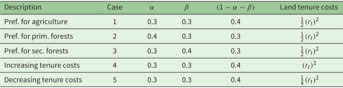
Equations (13) and (14) also tell us the deforestation and reforestation rates along the forest transition. Table 1 provides the parameters that differentiate various cases. Case 1 is the benchmark case, where the representative land user assigns more weight to agriculture and is indifferent between primary and secondary forests. This is the usual way development has proceeded in countries with forests. Other cases are used to examine the various drivers of the model. Notice that the variations of land tenure costs (cases 4 and 5) are built on the benchmark case (case 1). Indeed, a larger preference for agriculture, consistent with a lower $\alpha$ and $\beta$, is more prevalent in a developing economy, whose tenure is costly to secure unless land is cleared.

Table 1. Parameter values

4.1 Speed of deforestation and reforestation in the transition

From (10), the speed at which primary forests are deforested decreases with rents from primary forests, increases with preferences for agriculture (or agricultural rent), and increases with net marginal benefit of forest conversion. Equation (11) shows that the speed of reforestation increases with preferences for secondary forests (or secondary forests rent), decreases with preferences for agriculture, and decreases with marginal land tenure costs. From these results, the following proposition can be inferred:

Figure 2 illustrates these results. Referring to the benchmark case in the figure, agricultural land area surpasses 50 per cent of total land area by 100 time periods. The turning point occurs just before time period 150. While the initial stock of primary forest covers 80 per cent of total land, it ends up at a level of only 20 per cent after 200 time periods.

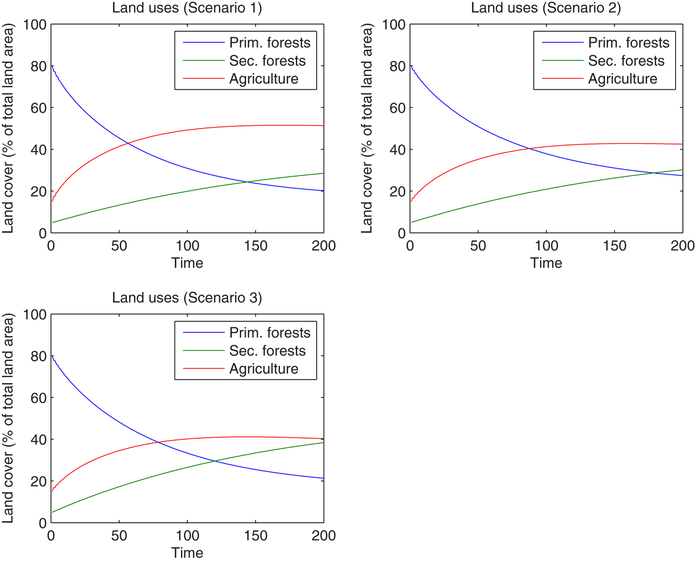
Figure 2. Variation in land uses under different preferences.

In cases 2 and 3, the relative preference is given to forests, either primary or secondary (see table 1). Overall, we note that deforestation proceeds more slowly than in the benchmark case. We also observe that case 2, when primary forests provide the highest rents relatively to agriculture and secondary forests, leads to a longer transition in time (i.e., later occurrence of a turning point) and this ultimately results in a preservation of more primary native forest cover. This suggests that while the period of net deforestation is longer, more biodiversity contained in primary forests is preserved.

4.2 Analyzing forest cover at the turning point

As described in section 2, the turning point is of particular importance in forest transition theory. At this point, net forest cover no longer decreases and reforestation compensates for deforestation. Two characteristics of the turning point can be considered in our model. The first is forest cover at the turning point, which gives an indication of the cumulative nature of deforestation during the development phase. Second, the time at which the turning point occurs is important as it indicates the length of the net deforestation (deforestation minus reforestation) phase.

The turning point takes place when the gain in secondary forest offsets the loss of primary forests, assuming that there is a unique point upon initial endowments, this takes place when $d_{t}=r_{t}$ and provided that $\Phi ^{\prime \prime }(r_{t})=C^{\prime \prime }(d_{t})=1$. Using this expression with (8) and (9) yields:

(15)\begin{equation} f^{\prime }(F_{t})+g^{\prime }(S_{t})=2h^{\prime }(1-F_{t}-S_{t})+\delta \lbrack p_{F}-C^{\prime }(d_{t})+\Phi _{t}^{\prime }(r_{t})]. \end{equation}

Equation (15) shows that the turning point between primary and secondary forests occurs when the double marginal return from agriculture equals the total marginal rents from all forest cover, minus the discounted profit from primary forest timber sale and the marginal cost of land tenure. This result is consistent with the scarcity path of the forest transition theory. Indeed, we see that the turning point occurs when the marginal value associated with forests equals that of converting.

As a conclusion, the forest stock at the turning point is higher when preferences and rents for primary and secondary forests are higher, and lower when timber price or preferences for agriculture are higher.

This result is confirmed by our simulations. It is straightforward to see from case 2 that the turning point occurs at a lower forest cover when preferences for agriculture are stronger. Propositions 1 and 2 therefore bring some interesting insights about the turning point: higher rents on primary forests decrease the speed of deforestation and postpone turning point occurrence, and they increase the forest stock once this turning point is achieved; higher rents on secondary forests, in contrast, imply that turning points are reached more quickly.

4.3 Role of land use and tenure costs to the length of the transition

In assessing transition length, our analysis uncovers two important issues: land-user preferences and land tenure costs. Another interesting piece of information comes from revisiting the length of the forest transition. From equation (15), ceteris paribus, a slower speed of deforestation indicates a longer transition, in the sense that it takes longer for the deforestation rate $d_t$ to equal that of reforestation $r_t$. The same type of reasoning can be made with reforestation: a slower speed of reforestation results in longer transition.

We can therefore reason that the length of forest transition increases with preferences for primary forests and decreases with the marginal benefit from primary forest conversion, since they decrease the speed of deforestation. Further, the forest transition length decreases with preferences for secondary forests and increases with marginal land tenure costs, which increase the speed of reforestation. Finally, the forest transition length may either increase or decrease with preferences for agriculture, since this increases both the speed of deforestation and decreases the speed of reforestation.

This result is visible in our simulations. Case 2 results in a lower rate of deforestation. In the same manner, when preferences for secondary forests are low, the reforestation rates are lower. Finally, when the preferences for agriculture are low, they tend to decrease the deforestation rate and to increase the reforestation rate. The combination of these three effects produces a longer forest transition.

In contrast, case 3 presents a relatively short forest transition. Here, higher preferences for secondary forests increase the speed of reforestation. Conversely, low preferences for primary forests increase the speed of deforestation. Lower agricultural preferences increase the reforestation rate and decrease the deforestation rate. In sum, a shorter forest transition results.

Our findings provide interesting and unexpected insights into the cumulative nature of deforestation. Indeed, when preferences for primary forests are higher, the net deforestation phase lasts longer, yet the cumulative amount of deforestation will be smaller. Thus, having positive net rates of deforestation is not necessarily critical for a country: it may simply mean that the forest transition phase will be longer, but with lower cumulative deforestation. In the same manner, high deforestation rates may suggest that the forest transition will appear more rapidly and potentially end with smaller cumulative deforestation. These are key results and suggest that the timing of policy aimed at reducing deforestation is much more complicated than previously thought.

The magnitude of tenure cost also influences the length of transition. Equation (15) and figure 3 illustrate this. The occurrence of the turning point is clearly affected by the land tenure costs. An increase in these costs (case 4) delays the turning point in forest cover relative to the reference case (case 1); the turning point occurs around 20 time periods later. On the contrary, not only does a decrease in these costs (case 5) significantly accelerate the occurrence of the turning point, but it appears at a time period with a higher total forest cover. This result is particularly relevant for public policies such as REDD+. Obviously, one way to accelerate transitions in developing countries is to reinforce property rights and political stability in order to decrease tenure costs.

Figure 3. Changes in land tenure cost.

In all, and from a long-term perspective, our model establishes that focusing only on current deforestation rates may be misleading in terms of predicting the final result of cumulative deforestation, and it is this final result that is of most interest to the rest of the world. We now provide an analysis of the steady states.

4.4 Steady-state analysis

Studying the steady state is of particular interest since it is likely that a given country reaches this condition after development. For example, France experienced its turning point during the 19th century, while the US reached its in the early 1900s, and the forest cover of both countries can therefore be considered as stationary from the perspective of the forest transition hypothesis.

Before the stationary point is reached, our model shows that clearing an additional hectare of primary forests provides $h^{\prime }(1-F_{t}-S_{t})+\delta \lambda _{t}$, while sustainable primary forests management gives $f^{\prime }(F_{t})+\dot {\lambda _{t}}$. Likewise, an additional hectare of secondary forests yields $g^{\prime }(S_{t})+\dot {\mu _{t}}$ while agriculture gives $h^{\prime }(1-F_{t}-S_{t})+\delta \mu _{t}$. The steady state is given by $\dot {F_{t}}=\dot {\lambda _{t}}=0$ and $\dot { S_{t}}=\dot {\mu _{t}}=0$. With $C^{\prime }(0)=\Phi ^{\prime }(0)=0$, in the steady state the marginal benefit from converting a hectare of natural old-growth forest is $\delta p_{F}+h^{\prime }(1-F_{\infty }-S_{\infty })$, which equals the marginal return from conserving primary forest $f^{\prime }(F_{\infty })$.

Concerning the dynamics of secondary forests, the steady state can be written as the equality of the marginal rents from a hectare of agriculture $h^{\prime }(1-F_\infty -S_\infty )$ and the marginal rents of a hectare of plantations $g^{\prime }(S_\infty )$. The representative agent is then indifferent between allocating an additional hectare of land either to agriculture or to the secondary forests.

Equalizing the steady states of the two types of forests by the marginal return from agriculture $h^{\prime }(1-F_{\infty }-S_{\infty })$ yields:

(16)\begin{equation} f^{\prime }(F_{\infty })-\delta p_{F}=g^{\prime }(S_{\infty }). \end{equation}

This result shows that, in the steady state, the marginal benefit from secondary forests equals that of primary forests minus the discounted sale price of timber obtained from clearing primary forests. This can be explained by the delay between the period of planting and realization of high ecosystem service benefits. Equation (16) implicitly also describes the tradeoff between primary and secondary forests. It follows that forest composition differs when preferences lean toward primary or secondary forests. As a result, total forest cover in the steady state is composed of both primary and secondary forests depending on the relative preferences for primary and secondary forests. Figure 4 provides some illustrative data on this point.

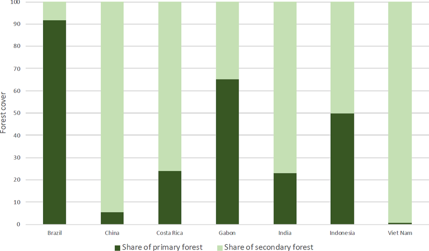
Figure 4. Forest composition in eight countries in 2010.

Costa Rica and Vietnam, which just passed the turning point, have a significantly different forest composition. According to the Forest Resources Assessment from FAO (Reference FAO2010), in Vietnam almost no primary forests were saved during the transition.Footnote ³ Since this type of forest can be viewed as a nonrenewable resource, its land area can only be equal or lower in the steady state. We can deduce the following proposition.

When primary forests are preferred, such as in cases 2 and 3, they represent a larger share of the forest cover in the long run. This result clearly indicates the validity and the importance of separately considering the dynamics of deforestation and reforestation as we do in our model. Indeed, when considering preferences for forests without distinguishing between their types, one would miss this composition effect. We can also argue that, despite similar total forest covers, case 2 is preferable in terms of biodiversity and carbon stocks, while case 3 better performs in terms of timber harvesting.

5.1 Reduction of land tenure costs

Consider the implication of a significant decrease in land tenure costs. Basically, we study a situation in which it is assumed that property rights are absent, as they are in frontier tropical forest areas where the transition is important, and where secondary forests are still considered a lower-valued use to agriculture by government laws. Thus, the costs of ‘tenure security’ that we use in our model represent costs that a private land user must spend to secure protection for various types of land; these costs are representative of what individual land users need to spend in order to protect their investments in the absence of property rights protections for forests by the government.

This type of reduction may come from the first phase of REDD+ implementation where strengthening tenure security is frequently mentioned as a key element before carbon redistribution. Moreover, previous results confirm that public policies should be targeted toward improving land institutions in order to retard deforestation (e.g., Bohn and Deacon, Reference Bohn and Deacon2000; Wolfersberger et al., Reference Wolfersberger, Delacote and Garcia2015).

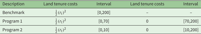
For this reason, we now revisit tenure costs in our model. We present two programs of public policies in complement to our benchmark case. Table 2 details the policy programs we examine.

Table 2. Parameter values for policy programs of land tenure cost reductions

For comparison purposes, preferences are assumed equal for the three cases, based on the benchmark ($\alpha =\beta$ $=0.3$ and $(1-\alpha -\beta )=0.4$). The first policy program is implemented halfway to the transition point and could correspond to countries such as Brazil or Indonesia. The second policy program is implemented earlier on the downward sloping arm of the forest transition curve, and could correspond to countries with a lower level of historical deforestation, such as the Democratic Republic of Congo or Gabon. The representative land user is assumed to face zero tenure costs under application of one of the programs.

Results are given in table 3. It is important to note here that numerical results have no significance per se (in terms of per hectare values for instance), but they are useful to give an idea on the qualitative interpretation of our model. Adding the shares of both types of forest at the end of forest transition ($t=200$), we find that programs 1 and 2 allow a country to preserve more total forest cover during development than in the benchmark case. This shows the effectiveness of the public policy. Also, when any program is implemented, net forest depletion halts earlier than in the benchmark (i.e., the turning point occurs earlier).

Table 3. The impact of reductions in tenure costs

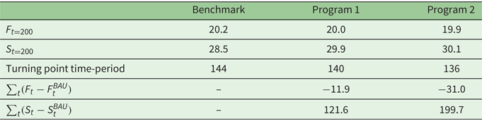
Two effects have to be distinguished. First, the policy has a direct effect of boosting reforestation. Since it is implemented at time period 10, program 2 always provides the best output in terms of reforestation. This therefore ends net emissions from forestry earlier than in the benchmark case. It is interesting to note the cumulative nature of reforestation here (last line of table 3). In terms of carbon balance, the second program is preferable to the first one, as the public policy of reforestation is set up earlier, which is more valuable in terms of carbon benefits. This result underlines the need to implement forest policies earlier during the transition, in order to benefit from the sequestration effect.

Second, the policy has an indirect effect on deforestation. Indeed, the more aggressive is the policy reform to tenure costs for reforestation (Program 2 $>$ Program 1 $>$ Benchmark), the lower is the amount of primary forests at the end of the transition ($t=200$). Also, the difference between the total area of primary forests with and without the program $\sum _{t}(F_{t}-F_{t}^{BAU})$ shows a loss of 11.9 and 31 land units in programs 1 and 2, respectively. These losses correspond to carbon releases due to deforestation. Then, under our assumptions, a public policy favoring reforestation also promotes deforestation of primary native forests. This corresponds to empirical observations. Given this indirect effect of the public policy, care must be exercised when designing a REDD+ strategy, since it can be harmful for primary native forests that have the highest ecological value.

Finally, examining welfare in the economy, we find logically that the earlier the program is implemented (i.e., the farther away from the transition), the higher is the level of welfare. This is explained by the fact that the REDD+ program removes a financial cost for the representative agent of the recipient economy. Assuming that the implementation of the program is costless for the representative land user, the difference in welfare between the economy under laissez-faire and the economy with REDD+ represents a social cost of not protecting the forests. The later the program is implemented, the higher is this cost.

5.2 Increasing the costs of deforestation

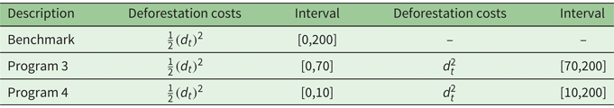
Now consider the implication of an increase in the cost of deforestation, $C(d_{t})$. We compare our BAU – business as usual – case with two cases where deforestation costs are double at different times. Table 4 details the policy programs we examine.

Table 4. Parameter values for policy programs of increasing deforestation costs

For comparison purposes, we keep preferences unchanged ($\alpha =\beta$ $=0.3$ and $(1-\alpha -\beta )=0.4$). The reform targeting primary forests is implemented at time period 10 and 70. The increase in the cost of deforestation may correspond to different possible actions, such as the implementation of protected areas, the use of monitoring/measuring, reporting, and verifying systems or an increase of decentralization associated with a higher control of corruption. It may also globally correspond to a reduction in access to primary forests, for example by framing the construction of new roads. Results are given in table 5.

Table 5. The impact of increasing deforestation costs

Again, the simulations allow us to identify both direct and indirect effects. Indeed, the rise in deforestation costs increases the stock of primary forests. For example, in Program 4, we find that compared to the benchmark, 378.9 units of primary forest cover are saved over the total transition. The indirect effect logically affects the stock of secondary forest, with a loss of 63.2 units reflecting the land use competition between the two forest types.

This is important to consider for REDD+, in order to reach the most valuable ecological outputs, depending on a country's context. Intuitively, in countries such as Guyana or the Democratic Republic of Congo, with a significant share of primary forests remaining, the REDD+ national strategy should target deforestation costs. Favoring plantations through a tenure cost reform could be harmful for old-growth natural forest that contains the largest quantity of biodiversity and carbon stock. Additionally, under some circumstances, policies to block deforestation in some areas can have positive spillovers leading to natural regeneration in surrounding areas, as Gandour (Reference Gandour2018) found for the Brazilian Amazon.

On the contrary, in countries where only a low quantity of primary forests remains, targeting deforestation costs would be ineffective. In those countries, a policy of land tenure costs reduction seems more appropriate. Eventually, it is important to keep in mind that despite the presence of an indirect effect, all policy programs lead to an increase in total forest area (primary and secondary forests taken together), and a decrease in total agricultural area, in comparison with the benchmark case.