1. Introduction
Marine fishery resources are under extreme pressure worldwide. According to recent studies (Garcia and Grainger, Reference Garcia and Grainger2005; FAO, 2010), three-quarters of fish stocks are maximally exploited or over-exploited. Moreover, the proportion of marine fish stocks which are intensively exploited is growing. Hence, sustainability is nowadays a major concern raised by international agreements and guidelines to fisheries management. Standard approaches to the sustainable management of fisheries such as MSY (maximum sustainable yield), MEY (maximum economic yield) or ICESFootnote 1 precautionary approaches usually address each exploited species separately (Grafton et al., Reference Grafton, Kompas and Hilborn2007). These management approaches have not succeeded in avoiding biodiversity loss, over-exploitation and fishing overcapacity worldwide (Hall and Mainprize, Reference Hall and Mainprize2004). The ecosystem approach for fisheries (EAF) or ecosystem-based fisheries management (EBFM) advocate an integrated management of marine resources to promote sustainability (FAO, 2003). Such a management policy requires first to account for the complexity of ecological mechanisms that encompass community dynamics, trophic webs, geographical processes and environmental uncertainties (habitat, climate). Furthermore, by putting emphasis on sustainability, this type of approach strives to balance ecological, economic and social objectives for present and future generations and to handle a large range of goods and services provided by marine ecosystems (Jennings, Reference Jennings2005), including both monetary and non-monetary values.
However, operationalizing the EBFM approach remains unclear and challenging. It requires models, indicators, reference points and adaptive management strategies. Plaganyi (Reference Plaganyi2007) provides an overview of the main types of modeling approaches and analyzes their relative merits for fisheries assessment in an ecosystem context. Modeling approaches and metrics useful for planning implementing and evaluating EBFM are also discussed in Marasco et al. (Reference Marasco, Goodman, Grimes, Lawson, Punt and Quinn2007), with particular emphasis on management strategy evaluation. The use of ecosystem indicators is analyzed by Rice (Reference Rice2000) and Cury and Christensen (Reference Cury and Christensen2005). In particular, Link (Reference Link2005) emphasizes the need for a multi-criteria approach to achieve ecological, economic and social objectives.
This article discusses the sustainable management of a multi-species and multi-fleet fishery from an ecosystem-based perspective for the small-scale fishery of French Guiana. Taking an EBFM approach to this case study was challenging. The fishery is characterized by various complex features including a high equatorial fish biodiversity impacted by several non-selective fleets and demographic growth which could potentially affect local food demand and consequently the production of this fishery.
2. Case study
The continental shelf of French Guiana is a tropical ecosystem under the influence of the Amazon estuary, as is the entire North Brazil Shelf Large Marine Ecosystem (LME) which contains a high biodiversity (Leopold, Reference Leopold2004). With 350 km of coastline, French Guiana benefits from a 130,000 km2 exclusive economic zone (EEZ) including 50,000 km2 of continental shelf. The coastal fishery operates 16 km offshore at depths of 0–20 m. Several landing points are spread along the coastline, and this fishery currently involves about 200 wooden boats locally named pirogues (P), canots créoles (CC), canots créoles améliorés (CCA) and tapouilles (T). Pirogues are canoes equipped with an outboard engine, which fish for periods of a few hours essentially in estuaries using ice stored in an old refrigerator. Compared to pirogues, Canots créoles are more adapted to sea navigation. Canots créoles améliorés have cabins and ice tanks which make it possible to fish for several days. Tapouilles are wider boats with a cabin and an inboard diesel engine. The gears used are drift or fixed nets, with mesh sizes between 40 and 100 mm. The type of fleet, the length of gill nets, the number of days spent at sea and the location of fishing activities all have an influence on the quantity of fish landed and on the species composition of the total harvest. Of the numerous coastal species, 30 are exploited and about 15 species, including weakfish, catfish and sharks, represent more than 90 per cent of the production. Annual landings have been estimated at approximately 2,700 tonnes for the past few years, as reported in the IfremerFootnote 2 Information System (http://www.ifremer.fr/guyane/Chiffres-cles).
The coastal fishery plays an important socioeconomic role for all the small towns along the coastline where more than 90 per cent of the population is located. However, assessment of this fishery only began in 2006 with data collection monitored by Ifremer. Production and fishing effort values are collected on a daily basis at the main landing points by observers from local communities. An exhaustive sampling is performed due to the small number of boats (approximately 200). Seventy five per cent of the fishing activity is observed on a daily basis from January to December. Each year, some 3,600 landings are recorded. For each landing, the production by species is estimated or weighed by the observers or reported by the fishermen. Other information is also collected, such as trip duration, net length and fishing area. Since the boats are under 12 m in length, fishermen are not obliged to provide this information. The data collection system depends significantly on the fishermen's collaboration. Economic assessment started in 2009 with a survey on production costs and selling prices carried out in the field. The coastal fishery in French Guiana remains largely informal despite: (1) the founding of the French Guiana fishers' cooperative (CODEPEG) in 1982; (2) the implementation of a system of professional licenses in territorial waters by the regional fisheries committee in 1995; and (3) the progressive application of national and European regulations (role of crew, safety inspections of boats, etc.). There is no quota for catches, and no limitation concerning exploited species and their size.
This coastal fishery provides an interesting case study from the perspective of EBF management. The current state of this fishery is usually postulated as safe, and the biodiversity associated with this resource does not seem to be threatened by fishing activity. Nevertheless, the sustainability of the fishery could be threatened by increasing local demand for fish linked to the demographic projections suggesting a 100 per cent increase in the local population over the next 20 years. Consequently, this increasing demand for local fish will affect fishing pressure. The question arises whether both the marine ecosystem and the fishing sector can cope with such changes and contribute to food security.
To examine these issues, this paper proposes a theoretical and empirical modeling of EBFM, using a multi-species and multi-fleet model integrating Lotka–Volterra trophic dynamics and profit functions. The dynamic model is calibrated on a monthly basis with 13 species and four fleets (P, CC, CCA and T) using catch and effort data from 2006 to 2009 derived from the Ifremer fishery information system. Ecological and economic performance of contrasting fishing scenarios including status quo, total closure, economic and viable strategies are examined and compared.
The main contribution of this work is two-fold. First, it proposes for the first time decision support tools for the management of the French Guiana coastal fishery by providing a bio-economic model, analysis and scenarios using time series on catch and fishing effort together with economic parameters. In the broader context of small-scale fisheries, such a bio-economic work relying on a perennial database is new to the best of our knowledge. It is acknowledged that small-scale fisheries are poorly managed due to a lack of tools and data adapted to their complexity, while these fisheries are crucial to sustaining many communities especially in developing or underdeveloped countries (Garcia et al., Reference Garcia, Allison and Andrew2008). The second contribution of this study is to advocate the use of co-viability approaches as a fruitful modeling framework for EBFM and sustainability issues. By accounting for complex and non-linear dynamics in a trophic and multi-fleet context and by addressing biodiversity issues, the paper shows that viability modeling (Bene et al., Reference Bene, Doyen and Gabay2001) can be applied to high- dimensional environmental systems. Moreover, this work points out that, by balancing ecological and economic goals with production and food security objectives over the next 40 years, the viability approach is well suited to coping with sustainability due to its multi-criteria perspective and the fact that it takes intergenerational equity into account, as in Péreau et al. (Reference Péreau, Doyen, Little and Thébaud2012).
The paper is structured as follows. Section 3 is devoted to the description of the ecosystem-based model together with bio-economic indicators and scenarios. Section 4 provides the calibration results and the outputs of the different fishing scenarios with respect to biodiversity and socioeco-nomic indicators. Results are discussed in terms of sustainability, EBFM and management tools in section 5. The final section provides a conclusion.
3. Methods
The numerical implementations of the model are carried out with the scientific software SCILAB 5.2.2.Footnote 3
3.1. The ecosystem-based model
Among the 30 exploited species, 13 were selected for the model as shown in table 1. These species represent 88 per cent of the total landing from 2006 to 2009. A virtual 14th species which stands for all the other marine producers was added. A potential trophic web (see figure a in the online appendix, available at http://journals.cambridge.org/EDE) was built with these selected species, according to their diet (Leopold, Reference Leopold2004) and their trophic level (table 1).
Table 1. The 13 selected species representing about 90% of the catches of the fishery

The ecosystem-based model is a multi-species, multi-fleet dynamic model described in discrete time with a monthly step. The states of the species in the ecosystem-based model are supposed to be governed by a complex dynamic system based on Lotka–Volterra trophic interactions and fishing efforts from the different fleets which play the role of controls in the system. Thus, at each step t, the biomass B i(t + 1) (kg) of species i at time t + 1 depends on other stocks B j(t) and fishing efforts e k(t) of fleet k (time spent at sea, in hours) through the relation:
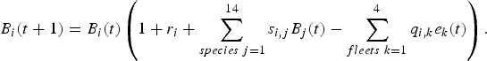 $$B_{i}\lpar t+1\rpar =B_{i}\lpar t\rpar \left(1+r_{i}+\sum_{species\, j=1}^{14}s_{i\comma j}B_{j}\lpar t\rpar -\sum_{fleets\ k=1}^{4}q_{i\comma k}e_{k}\lpar t\rpar \right).$$
Here r i stands for the intrinsic growth rate of the population i and s i, j the trophic effect of species j on species i (positive if j is a prey of i and negative if j is a predator of i). The parameter q i, k measures the catchability of species i by fleet k. It corresponds to the probability of a biomass unit of species i being caught by a boat of fleet k during one fishing effort unit. The number of the fleet k from k = 1 to k = 4 corresponds respectively to CC, CCA, P and T.Footnote 4
The catches H i, k of species i by fleet k at time t are thus given by the Schaefer production function:
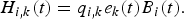 $$H_{i\comma k}\lpar t\rpar = q_{i\comma k}e_{k}\lpar t\rpar B_{i}\lpar t\rpar .$$
3.2. Model and calibration inputs
Values used to define the model parameters came from different sources. Daily observations (catches and fishing efforts) from the landing points all along the coast are available from January 2006 to December 2009. Every month during this 48-month period, for each of the four fleets, fishing effort and catches were identified for the 13 species, for a total of 2,688 observations. The literature (Leopold, Reference Leopold2004) and FishbaseFootnote 5 provided qualitative trophic interactions concerning the sign of the relationship between species and intrinsic growth rates to start the calibration. In particular, only prey–predator and mutual competition relationships are considered in the Lotka–Volterra model, and not symbiotic relationships between species. Initial stocks, catchabilities, trophic intensities and refined intrinsic growth rate values of this ecosystem were estimated through a least square method. This method consisted of minimizing the mean square error between the monthly observed catches  $H_{i\comma k}^{{\rm data}}$ and the catches H i, k simulated by the model, as defined by equations (1) and (2):
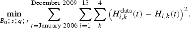 $$\min_{B_{0}\semicolon \, s\semicolon \, q\semicolon \, r}\sum_{t={\rm January}\ 2006}^{{\rm December}\ 2009} \sum_{i=1}^{13}\sum_{k}^{4}\big(H_{i\comma k}^{{\rm data}}\lpar t\rpar -H_{i\comma k}\lpar t\rpar \big)^{2}.$$
 Here  $\lpar B_{0}\semicolon \; \ s\semicolon \; \ q\semicolon \; \ r\rpar $ is the set of parameters to identify. B 0 = B(t 0) is the vector (14 × 1) of initial stocks (t 0= December 2005), s the matrix
  $\lpar 14\times14\rpar$ of trophic interactions, q the matrix (14 × 4) of catchabilities, and r a vector (14 × 1) of intrinsic growth rates.
Several simple biological and productive constraints on parameters were taken into account for the optimization process (equation 3). In particular, several intra-specific interaction coefficients were set to zero (typically B.catfish, F.mullet and P.mullet, i = 10, 12, 13), prey–predator relationships (A. weakfish serve as prey for sharks s 5, 1 > 0 and sharks are predators of A. weakfish s 1, 5 < 0), common prey relationships (A. weakfish also serve as prey for G. groupers s 11, 1 > 0) and mutual competition (the predators shark and G. grouper prey on each other, s 5, 11 < 0 and s 11, 5 < 0) were considered (table a, online appendix). Some catchability parameters q i, k were also set at zero since some species are not caught by fleets, typically fleet T (table b, online appendix). The non-linear optimization problem (equation 3) was solved numerically using the Scilab routine entitled ‘optim_ga’ which relies on an evolutionary (or genetic) algorithm.Footnote 6
3.3. Model outputs: ecological indicators
After calibration, ecological and economic indicators were computed to assess the performance of both the ecosystem and the fishery. We first focused on biodiversity indices. Although the choice of a biodiversity metric remains controversial as pointed out in Magurran (Reference Magurran2007), we selected the species richness, Simpson and marine trophic indicators provided by equations (4), (5) and (6).
3.3.1. Species richness
Species richness SR(t) indicates the estimated number of species represented in the ecosystem. It is measured by an indicator function based on abundances N i(t), computed as the ratio between the biomass B i(t) and the common weight w i of each species, derived from the Fishbase information system:
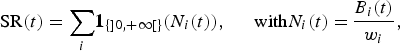 $${\rm SR}\lpar t\rpar = \mathop {{\sum_i} {\bf 1}_{\lcub ] 0\comma + \infty [ \rcub } \lpar N_i \lpar t\rpar \rpar \comma \; \, \quad {\rm with} N_i \lpar t\rpar = }\displaystyle{{B_i \lpar t\rpar } \over {w_i }}\comma$$
where the function  ${\bf 1}_{\lcub ] 0\comma +\infty [ \rcub }$ corresponds to the characteristic functionFootnote 7 of positive reals. Thus, it is assumed that a species disappears whenever its abundance falls to zero (Worm et al., Reference Worm, Barbier and Beaumont2006). It should be noted that rare species have a relatively huge impact on the species richness index.
3.3.2. Simpson's diversity
The Simpson index SI(t) is expressed as:
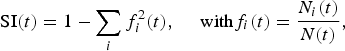 $${\rm SI}\lpar t\rpar =1-\sum_{i}f_{i}^{2}\lpar t\rpar \comma \; \quad {\rm with} f_{i}\lpar t\rpar =\displaystyle{{N_i\lpar t\rpar } \over {N\lpar t\rpar }}\comma$$
where  $N\lpar t\rpar =\sum\limits_{i}N_{i}\lpar t\rpar$. The index SI estimates the probability of two individuals belonging to the same species. The index varies between 0 and 1. A perfectly homogeneous community would have a Simpson diversity index score of 1. Such a metric gives more weight to the more abundant species. The addition of rare species causes only small changes in the value.
3.3.3. Marine trophic index
The trophic level indicates the location of a species in a food web, starting with producers (e.g., phytoplankton, plants) at level 0, and moving through primary consumers that eat primary producers (level 1) and secondary consumers that eat primary consumers (level 2), and so on. In marine fishes, the trophic levels vary from two to five (top predators). The marine trophic index MTI(t) of the ecosystem (Pauly and Watson, Reference Pauly and Watson2005) is computed from the trophic level of each species T i (table 1) and their relative abundances f i (see equation 5):
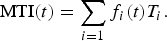 $${\rm MTI}\lpar t\rpar =\sum_{i=1}f_{i}\lpar t\rpar T_{i}.$$
3.4. Model outputs: economic indicators
We now turn to the assessment of the fishing sector through production and profitability values of the fishery provided by equations (7) and (8).
3.4.1. Food supply
We first considered the total catches H(t) within the fishery which play the role of food supply:
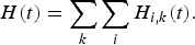 $$H\lpar t\rpar =\sum_{k}\sum_{i}H_{i\comma k}\lpar t\rpar .$$
This supply must be compared with local food demand, which is expected to increase at an exogenous rate provided by demographic scenarios and projections over the next 20 years.
3.4.2. Profits
The profit πk(t) of each fleet k was derived from the landings of each species H i, k, the landing prices p i, k, fixed costs  $c_{k}^{f}$, variable costs
  $c_{k}^{v}$ and the crew share earnings βk as follows:
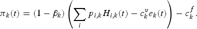 $$\pi _{k}\lpar t\rpar =\lpar 1-\beta _{k}\rpar \left(\sum_{i}p_{i\comma k}H_{i\comma k}\lpar t\rpar -c_{k}^{v}e_{k}\lpar t\rpar \right)-c_{k}^{f}.$$
 Prices, variable costs and fixed costs are those collected for 2008 (table c, online appendix). They were assumed to remain unchanged throughout the simulations. Share contract β is the salary system commonly used in this fishery for the CCA fleet (k = 2) and T fleet (k = 4). Crews are remunerated with a share of the landing value minus the variable costs. CC fleet (k = 1) and P fleet (k = 3) crews are mostly made up of boat owners, occasionally assisted by a family member. If there is a pay system for these fleets, it differs from one owner to another. Hence, to simplify, we set βk = 0 for CC and P fleets and βk = 0.5 for CCA and T fleets. Variable costs  $c_{k}^{v}$ include fuel consumption, ice, food and lubricants. Equipment depreciation, maintenance and repairs are incorporated in the fixed costs
  $c_{k}^{f}$.
The total profit π(t) is the sum of profits over all fleets:
 $$\pi\lpar t\rpar = \sum_k \pi_k\lpar t\rpar .$$
3.5. Fishing scenarios
From the calibrated model, scenarios were simulated according to different fishing efforts over 40 years. We distinguished four scenarios: closure (CL), status quo (SQ), economic (PV) and co-viability (CVA). The set of ecological and economic indicators introduced previously were evaluated for these four scenarios.
3.5.1. The closure scenario (CL)
The CL scenario corresponds to the implementation of a no fishing zone over the whole French Guiana coastal area:
 $$e_k \lpar t\rpar = 0\comma \; \quad \forall k=1\comma \; \ldots \comma \; 4\quad \forall t=t_{1}\comma \; \ldots \comma \; t_{f}$$
where t 1 corresponds to January 2010 and t f to December 2050.
3.5.2. The status quo scenario (SQ)
The SQ scenario simulates a steady fishing effort based on the mean pattern of the efforts between 2006 and 2009:
 $$e_{k}\lpar t\rpar =\overline{e}_{k}\comma \; \quad \forall k=1\comma \; \ldots \comma \; 4\quad \forall t=t_{1}\comma \; \ldots \comma \; t_{f}$$
with  $\overline{e}_{k}$ representing the mean efforts between 2006 and 2009 for the fleet k as follows:
 $$\overline{e}_{k}=\displaystyle{{1} \over {t_{1}-1}}\sum_{t=t_{0}}^{t_{1}-1}e_{k}\lpar t\rpar \comma \;$$
where t 0 and t 1 − 1 correspond to January 2006 and December 2009, respectively.
3.5.3. The economic scenario (PV)
The PV scenario maximizes the present value of all the future profits aggregated among the fleets π (t) defined by equation (9). The present value depends on fishing effort patterns as follows:
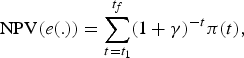 $${\rm NPV}\lpar e\lpar .\rpar \rpar =\sum_{t=t_{1}}^{t_{f}}\lpar 1+\gamma \rpar ^{-t}\pi \lpar t\rpar \comma \;$$
where γ is the discount rate set at γ = 3 per cent. The optimal program underlying the PV scenario is defined by
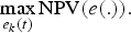 $$\max_{e_{k}\lpar t\rpar }{\rm NPV}\lpar e\lpar .\rpar \rpar .$$
 In this scenario, it is assumed that the fishing efforts e k(t) rely on a control strategy that can be adapted every 5 years.Footnote 8 In other words, eight decisions  $\lpar e_{k}\lpar t_{1}\rpar \comma \; e_{k}\lpar t_{2}\rpar \comma \; \ldots \comma \; e_{k}\lpar t_{8}\rpar \rpar $ are available for each fleet k as follows:
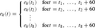 $$e_{k}\lpar t\rpar = \left\{\matrix{ e_{k}\lpar t_1\rpar & {\rm for} t=t_1\comma \; \ldots\comma \; t_1+60 \cr e_{k}\lpar t_2\rpar & {\rm for}t=t_2\comma \; \ldots\comma \; t_2+60 \cr \quad\vdots \cr e_k\lpar t_8\rpar & {\rm for}t=t_8\comma \; \ldots\comma \; t_8+60} \right.$$
where t 1 and  $t_{n}=t_{n-1}+60$, for n = 2 to 8, are decisive months.
The optimal effort e k(t) solutions of the intertemporal program (equation 11) were approximated numerically by again using an evolutionary algorithm, in particular the routine entitled ‘optim_ga’ in Scilab.
3.5.4. The co-viability scenario (CVA)
The purpose of the CVA scenario is to provide a satisfactory balance over time between fleet profitability, biodiversity and local food demand. Thus, viable levels of fishing effort aim at complying with the bio-economic constraints below:
• A profitability constraint:
 $\pi_{k}\lpar t\rpar \geq 0\comma \; \ \forall t=t_{1}\comma \; \ldots\comma \; t_{f}\comma \; \ \forall k=1\comma \; \ldots\comma \; 4$
• A species richness constraint:
${\rm SR}\lpar t\rpar \geq 11\comma \; \ \forall t=t_{1}\comma \; \ldots\comma \; t_{f}$• A food security constraint:
$H\lpar t\rpar \geq H\lpar 2009\rpar \cdot \lpar 1+d\rpar ^{t}\comma \; \ \forall t=t_{1}\comma \; \ldots \comma \; t_{f}$,


where d stands for the growth rate of the population. The profitability constraint holds for each fleet separately and not for the aggregated rent as in the PV scenario. Concerning the biodiversity constraint, no co-viability path maintaining the whole set of 13 species was exhibited. This explains why the species richness required was relaxed to only 11 species. Finally, the food security constraint assumed an increase in the local fish demand at the annual rate of d = 3 per cent, according to the demographic scenario which predicts a doubling of French Guiana's population by 2030 (INSEE, 2011). Moreover, it was assumed that fish species can be substituted, in the sense that a drop in the consumption of one species can be compensated for by a rise in the consumption of other species.
Following DeLara and Doyen (Reference De Lara and Doyen2008) and Doyen and De Lara (Reference Doyen and De Lara2010), viable efforts for the CVA scenario were obtained by maximizing the following criterion:
 $$\max_{e_k\lpar t\rpar }\prod_{t=t_1}^{t_f}{\bf 1}_{\lcub ] 0\comma +\infty [ \rcub } \lpar \pi _k\lpar t\rpar \rpar {\bf 1}_{\lcub ] 0\comma +\infty [ \rcub } \lpar {\rm SR}\lpar t\rpar -11\rpar {\bf 1}_{\lcub ] 0\comma +\infty [ \rcub }\cdot \lpar H\lpar t\rpar -H\lpar 2009\rpar \cdot \lpar 1+d\rpar ^{t}\rpar$$
where again, efforts e k(t) are meant to be control strategies that can change every 5 years as in equation (12), and  ${\bf 1}_{\lcub ] 0\comma +\infty [ \rcub }$ represents the characteristic function on positive reals. The numerical method again relies on the evolutionary optimization routine.
3.6. Sensitivity analysis and uncertainty margins
A sensitivity analysis was carried out to evaluate the role played in the bio-economic outputs by the different calibrated parameters (tables a and b, online appendix). To achieve this, we ran additional simulations based on the SQ scenario. Given the large number of parameters, we limited the sensitivity analysis by simultaneously perturbing all the parameters of the same group, i.e., initial stocks B 0, catchabilities q, trophic intensities s and intrinsic growth rates r. For each group of estimated biological parameters, a noise ranging from −10 per cent to +10 per cent of the calibrated values was added to the parameters. The relative differences in bio-economic outputs including average catches per annum  $\overline{H}=\displaystyle{{12} \over {t_{f}-t_{1}}}\sum\limits_{t=t_{1}}^{t_{f}}H\lpar t\rpar $, net present value (NPV) and specific richness SR(t f) were computed. Sensitivity analysis was also carried out to examine the impact of the choice of time horizon on the outputs. Therefore, other simulations with the SQ scenario were performed, increasing the simulation length t f from December 2060 to December 2100. The corresponding bio-economic results were compared with those obtained with
  $t_f={\rm December}$ 2050.
In line with this, in order to assess the reliability of the outputs for each effort scenario, simulations were replicated 400 times by introducing uncertainties in the estimated parameters (r, s, q, B 0). For each simulation, a noise ranging from −10 per cent to +10 per cent of the calibrated values was again randomly added to the parameters.
4. Results
4.1. Calibration and sensitivity results
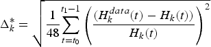
Figure 1 presents the historical and simulated catches by fleet, with 95 per cent confidence intervals. For each fleet k, confidence intervalsFootnote 9 were computed from the mean relative errors Δk between observed and simulated catches from January 2006 to December 2009,
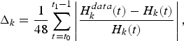 $$\Delta _{k}=\displaystyle{{1} \over {48}}\sum_{t=t_{0}}^{t_{1}-1}\left\vert \displaystyle{{H_{k}^{data}\lpar t\rpar -H_{k}\lpar t\rpar } \over {H_{k}\lpar t\rpar }}\right\vert\comma \;$$
where  $H_{k}\lpar t\rpar =\sum_{i}H_{i\comma k}\lpar t\rpar $ stands for catches by fleet k at time t over the whole 13 species i. The mean relative errors equalFootnote 10
 $\Delta _{1}=0.259$ for CC,
  $\Delta _{2}=0.13$ for CCA,
  $\Delta _{3}=0.354$ for P and
  $\Delta _{4}=0.176$ for T.

Figure 1. Comparison by fleet k between historical catches  $\displaystyle \sum_{{\rm species} i}H^{{\rm data}}_{{\rm species} i\comma k}\lpar t\rpar $ (solid lines) and simulated catches
  $\displaystyle \sum_{i}H_{i\comma k}\lpar t\rpar $ (dashed lines), with the confidence intervals at 95% (dotted lines)
Figure 2 displays the sensitivity results. They stress the fact that the parameters with the greatest impact were intrinsic growth rates r i and trophic interactions s ij. The relative changes in NPV and average catch outputs appear to be approximately linear functions of the perturbations with slopes between 0 and 1.8 highlighting bounds for the marginal effects of the parameters. In particular, the impact of initial biomasses was small since the relative changes were less than the perturbation magnitude for these biomasses. Trophic intensities and intrinsic growth rates were the inputs for which a perturbation entailed larger relative changes in the outputs. The non-linear nature of the species richness index is captured by the staircase shape of the relative change as well as the peaks observed. Moreover, the relative changes in bio-economic outputs in comparison to the 2050 time horizon show a reduced impact of the temporal target in the results. In particular, the NPV is not affected by a change of horizon mainly because of the discount involved. Of interest is the fact that species richness is stabilized after 2070. The average annual catches continue to rise with the time horizon, which emphasizes the fact that overall fishery production does not collapse after year 2050 and could even be enhanced.

Figure 2. Relative changes of NPV (solid line), average annual catches  $\overline{H}$ (dotted line), species richness SR(t f) (dashed line), according to variations in input parameters by 1% increments from − 10% to + 10% (a, b, c and d), and time horizon (e). The baseline is status quo scenario SQ
4.2. Scenarios, effort levels
Figure 3 displays the effort multipliers  $\displaystyle{{e_k\lpar t\rpar } \over {\overline {e}_k}}$ by fleet for each fishing scenario. These effort multipliers are based on the comparison between effort e(t) and the mean pattern of efforts
  $\overline{e}_{k}$ between 2006 and 2009 defined in equation (10). The SQ effort multiplier is equal to one, as expected. It turns out that the PV scenario induces the largest decrease in fishing efforts to maximize the present value of aggregated rent. In particular, the PV scenario implies stopping fishing activity for the CC and CCA fleets during the entire simulation period. With regard to the T fleet, fishing effort is increased in the first two decades of the simulation and stopped in the last decade. By contrast, the fishing effort of the P fleet follows an opposite pattern. Effort is nil during the first two decades of the simulation and is increased after 2030. The multiplier for the T fleet reaches 2.4 in the first part of the simulation, while for the P fleet, multipliers range from 2.2 to 7.8 for the second part of the simulation. In contrast, the CVA scenario guarantees an activity for every fleet throughout time. On average, its effort level is lower than the baseline SQ except for the T fleet, which exhibits an effort multiplier ranging from 0.9 to 6.8. The average multiplier of the viable strategy is 0.7 for CC, 0.51 for CCA, 0.75 for P and 3.0 for T.

Figure 3. Fishing effort multiplier  $u_{k}\lpar t\rpar =\displaystyle{{e_{k}\lpar t\rpar } \over {\overline{e_k}}}$ by fleet and scenario: SQ (solid line), economic PV (dotted line), co-viability CVA (dashed line)
4.3. Ecological results
Trends in the evolution of species richness according to the scenarios are plotted in figure 4 (marine trophic and Simpson diversity evolutions are available in figures b and c in the online appendix). The ‘mean’ trajectories induced by the calibrated values are plotted together with margin errors of 400 simulations derived from the perturbation of the parameters selected randomly in  $[ -10\hbox{ per cent}\semicolon \; +10\hbox{ per cent}] $. First it appears that a loss of species occurs for every scenario, as species richness decreases in every case except in the CL scenario, as expected (at least when the parameters are not perturbed). In other words, implementing a no fishing zone should maintain species diversity. By contrast, the baseline SQ scenario leads to the worst result in terms of diversity loss. Species richness ranges from 11 to 8 at the end of the simulation period. The mean simulation provides nine species at the end and species like Crucifix catfish, Common snook, Silver croaker and Bressou catfish disappear. With the PV scenario, both Crucifix catfish and Bressou catfish collapse. The final state of species richness with the CVA scenario is qualitatively identical to the PV scenario since 11 species remain at the end while the same species disappear. From mean estimated parameters, two species (Crucifix catfish and Bressou catfish) become extinct in the SQ, CVA and PV scenarios, but the extinction periods are not identical: species extinctions are delayed in proportion to the reductions in effort level. Extinction periods of these two species correspond to years 2020–2032 for the SQ scenario, 2022–2040 for the CVA scenario and 2031–2047 for the PV scenarios respectively.

Figure 4. Species richness SR(t) evolution by scenario (solid lines), with uncertainties (vertical lines)
The trajectories of the two other biodiversity indices are more complex and difficult to interpret. The species abundances change considerably in the simulation period. In particular, a major change occurs around 2015 for all ecological indicators when certain species start to decline. This decrease is illustrated by the decline in catches between 2015 and 2020 for the SQ scenario (figure 5). At the start of the mean simulation, the total biomass is not equally distributed among the species with SI = 0.5, and the marine ecosystem is dominated by species with a low trophic level, MTI = 2.5. At the end of the mean simulation, for all scenarios, diversity indices are better than those at the beginning (SI ranges from 0.61 to 0.77, MTI from 2.79 to 3.08, according to the scenario).

Figure 5. Total catches H(t) by scenarios (solid lines) vs. local fish demand (dashed line), with uncertainties (vertical lines)
The impact of uncertainties is significant, as the ecological indices appear volatile in particular for the last years. This indicates that the results should be considered with caution.
4.4. Economic results
Catches and profits for the SQ, PV and CVA scenarios are plotted in figures 5–8. The main biomass changes in years 2015–2020 also affect the catches and profits. The SQ scenario seems economically viable in terms of profitability, as annual profits are positive during almost the entire period for all fleets. However, exceptions occur for the CC and CCA fleets in the first years of the simulation and for the P fleet in the 2010–2011 and 2026–2034 periods. Not surprisingly, the PV scenario yields the highest cumulative discounted profit, between € 1.125 and 2.399 billion vs. €123.2–203.3 million vs. for the SQ scenario and € 84.7–239.9 million for the CVA scenario. The greatest fishing activity occurs in the second part of the simulation for the P fleet. One explanation can be found in the high value of the selling prices for this fleet (table c, online appendix). On average, the CVA scenario provides positive annual profits for each fleet throughout the simulation despite the fact that the CVA fishing effort is lower than the SQ effort. However, as the CVA scenario effort levels were computed from the mean estimated parameters, the uncertainties may alter the profitability in certain years.

Figure 6. Profit πk(t) by fleet for the SQ scenario (solid lines), with uncertainties (vertical lines). The dotted line stands for profitability threshold

Figure 7. Profit πk(t) by fleet for the PV scenario (solid lines), with uncertainties (vertical lines). The dotted line stands for profitability threshold

Figure 8. Profit πk(t) by fleet for the CVA scenario (solid lines), with uncertainties (vertical lines). The dotted line stands for profitability threshold
Comparison of the fish demand curve with the supply curves by scenario (figure 5) shows that yield levels may differ broadly from local fish demand projections. In particular, for a period of several years, the mean production is lower than the fish demandFootnote 11 except for the mean CVA scenario, as expected. In the same vein, the mean cumulative supply over 40 years of the CVA scenario with  $H=\sum_{t}H\lpar t\rpar \approx 262$ Ktons is the closest to the cumulative fish demand of 144 Ktons as compared to the SQ and PV scenarios with H = 284 and H = 986 Ktons respectively. However, it also appears that the food security constraint of the CVA scenario may be violated during some years when uncertainties are taken into account.
5. Discussion
5.1. Co-viability as a step towards sustainability
Let us first analyze our results in terms of sustainability. Obviously, a total fishery closure is not a satisfactory solution either economically or socially in terms of jobs, income and food consequences. It turns out that maintaining constant efforts through the SQ scenario is also not a suitable and sustainable strategy. In fact, aside from the fact that the CC and P fleets do not realize any profit in the first years, the SQ scenario does not satisfy the constraint of local consumption from years 2028–2038 in the mean regime and provides the worst performance for species richness. The calibration context can partially explain the negative profits of these fleets at the beginning of the simulation. Indeed, economic data are based on year 2008 which was unusual: fuel prices reached a record and thus production costs rose considerably. More generally, the low prices at first sale and the production costs did not allow every vessel to generate profits. Not surprisingly, the largest cumulative discounted profit and the most important fish supply are obtained with the PV scenario. However, this scenario may not be socially acceptable since profits are not evenly distributed between fleets over time. This happens because this scenario imposes that the CC and CCA fleets cease their activities, inducing negative profits for these fleets due to fixed costs (figure 7). That some fleets exhibit negative profits is consistent from the social planner's point of view underlying the PV approach, since aggregated profits are optimized by favoring the most efficient fleets. A better balance between biodiversity and socioeco-nomic performance can be reached with the CVA scenario, at least on average. Although two species disappear, this scenario appears to be the best compromise: it allows annual positive mean profits for every fleet and satisfies local consumption during the 40 years of simulation. However, the variability of outputs due to noise in parameters suggests that a stochastic or robust approach would be fruitful to guarantee this viability in an uncertain context.
In addition to analysis on the case study, this work advocates an integrated and multi-criteria approach. A wide range of stakeholders are involved in fisheries, including: industrial, artisanal, subsistence and recreational fishermen; suppliers and workers in allied industries; managers, environmentalists, biologists, economists; public decision makers and the general public. Each of these groups has an interest in particular outcomes from fisheries, and the outcomes that are considered desirable by one stakeholder may be undesirable for another group (Hilborn, Reference Hilborn2007). Considering this multi-dimensional nature of marine fisheries management is a way to guarantee the reasonable exploitation of aquatic resources, allowing the creation of conditions for sustainability from economic, environmental and social viewpoints. The present work is fully in line with these considerations. First, of interest is the use of bio-economic models and assessments articulating ecological and socioeconomic processes and goals as in Bene et al. (Reference Bene, Doyen and Gabay2001); Doyen et al. (Reference Doyen, Thébaud and Béné2012); Péreau et al. (Reference Péreau, Doyen, Little and Thébaud2012). Moreover, by focusing on sustainability and viability, the present model exhibits management strategies and scenarios that account for intergenerational equity. As emphasized in Martinet and Doyen (Reference Martinet and Doyen2007) and DeLara and Doyen (Reference De Lara and Doyen2008), viability is closely related to the maximin (Rawlsian) approach with respect to intergenerational equity. In this respect, the CVA strategy turns out to be a promising approach.
5.2. Co-viability as a step towards EBFM
Several authors have proposed the viability approach as a new, innovative and well-suited modeling framework for EBFM (Cury et al. Reference Cury, Mullon, Garcia and Shannon2005; Doyen et al. Reference Doyen, Thébaud and Béné2012). They argue that the viability approach, especially co-viability, is relevant in handling EBFM issues because it may simultaneously account for dynamic complexities, bio-economic risks and sustainability objectives balancing ecological, economic and social dimensions for fisheries. In particular, Cury et al. (Reference Cury, Mullon, Garcia and Shannon2005) and Doyen et al. (Reference Doyen, De Lara, Ferraris and Pelletier2007) show how the approach can potentially be useful for integrating ecosystem considerations for fisheries management. Mullon et al. (Reference Mullon, Cury and Shannon2004), Bene and Doyen (Reference Bene and Doyen2008) and Chapel et al. (Reference Chapel, Deffuant, Martin and Mullon2008) emphasize the ability to address complex dynamics in this framework. The computational and mathematical modeling methods proposed in this paper through the CVA strategy are motivated by a similar prospect. One major advantage of the co-viability approach is the fact that the viability framework is dynamic and thus makes it possible to capture the interactions and co-evolution of marine biodiversity and fishing. The dynamics can potentially include complex mechanisms such as trophic interactions, competition, metapopulation dynamics or economic investment processes. Here the focus is both on trophic and technical interactions through a multi-fleet and multi-species context as in Doyen et al. (Reference Doyen, Thébaud and Béné2012).
Projections over 40 years for different fishing scenarios highlight the complexity of mechanisms at play, particularly their non-linearity. With regard to this point, the trajectories of ecological indicators are representative and should not be interpreted separately. The species richness for the CL scenario can be sustained, meaning that all species are present at the end of the mean simulation. However, the Simpson and marine trophic indices reveal that species abundances change over the simulation period, even more when uncertainties on estimated parameters are considered. Diversity index (SI, MTI) values at the end of the mean simulation lead to the following findings: (1) total biomass is better distributed among species and (2) the species with a high trophic level are better represented. Thus, the effects of fishing on the species can be deduced: fishing leads to ecosystem specialization.
5.3. Decision support for the French Guiana small-scale fishery
Small-scale fisheries remain poorly managed because of their heterogeneity, difficulties in getting consistent and perennial data and the lack of regulation tools. The problem is more acute in a tropical context with a high-level informal activity and high biodiversity with low stock biomass (this is typically valid for reef ecosystems). In French Guiana, waters are very turbid and productive due to the proximity of the Amazon river. There are no reefs, but biodiversity is high, as is biomass. The bio-economic database monitored from 2006 with the help of local communities who collected time series data offers the opportunity to go a step further towards building management tools. Since the decline of the French Guiana industrial shrimp fishery (Chaboud et al., Reference Chaboud, Vendeville, Blanchard and Viera2008), the coastal fishery has become a sector with a high potential for development. In 2008, coastal fishery production was higher than shrimp and red snapper landings. However, as previously stated, there is no quota for catches, and no limitation concerning exploited species and their size. Regulation tools are derived from commonly used national and European fisheries management systems. These standards concern the gear selectivity (mesh size) and the global size of the fleet through total engine power and total vessel capacity. However, due to the lack of studies on the stock status for the main exploited species, rules relating to overall fleet size have not been adapted to the changing level of fish stocks. The only aim of the current management strategy is to prevent fishing activity by unauthorized boats. The present bio-economic study should contribute to the design of more scientific and relevant assessments and regulations for both the marine ecosystem and this small-scale fishery. At this stage, we would like to point out the methodological interest of sustaining the fishery information system to achieve such goals.
Fishing scenario outputs show that fishing performance, including food supply and profitability of fleets, can be increased or sustained. In particular, this suggests that the marine ecosystem and the fishing sector could cope with food demand and contribute to food security. This could have positive consequences for the development of French Guiana, since the coastal fishery plays an important socioeconomic role for the small towns along the coastline where more than 90 per cent of the population is located. However, there is a risk of losing fish biodiversity due to fishing pressure. This loss of biodiversity could potentially alter some ecosystem services (not taken into account in the current model) and the outcomes of the fishery itself in the long run. Thus, some fish stocks should be evaluated more specifically in order to anticipate their depletion (Crucifix catfish, Bressou catfish). Depending on the endangered stocks, conservation measures for the productive and reproductive capacities of these stocks should be taken. This could be achieved by banning fishing in nursery areas or providing incentives for using more selective fishing techniques. In this way, the co-viability approach could enable long-term management of the French Guiana coastal fishery. The CVA scenario suggests that such a multi-functional sustainability would be maintained with a small increase in the T fleet's effort and a relative reduction for the other fleets (CC, CCA or P). This management strategy entails implementing limitations on fishing effort. Nevertheless, this scenario may remain attractive for the different stakeholders involved since the profitability constraint for each fleet, the species richness constraint and the food security constraint are all satisfied. In this sense, the CVA strategy could be potentially operationalized with the fishermen's cooperation.
6. Conclusion
This work provides a bio-economic model and analysis for the coastal fishery in French Guiana. It relies on a multi-species and multi-fleet model integrating Lotka–Volterra trophic dynamics and profit functions. The dynamic model is calibrated using data from the Ifremer fishery information system. Ecological and economic performance of contrasting fishing scenarios including status quo, total closure, economic and viable strategies are compared. The major contribution of the paper is two-fold. First, it proposes for the first time decision support tools for the management of the small-scale fishery in French Guiana. Small-scale fisheries are poorly managed due to a lack of tools and data, although these fisheries are crucial to sustaining many communities especially in developing or underdeveloped countries (Garcia et al., Reference Garcia, Allison and Andrew2008). The present work emphasizes the interest of bio-economic models which rely on a perennial database in this context of small-scale fisheries. The second contribution of this study is to advocate the use of viability approaches as a relevant modeling framework for EBFM and sustainability issues. Such sustainability is known to be difficult to achieve because economic, social and ecological goals can contradict each other (Pitcher, Reference Pitcher2001). The paper points out that, by balancing ecological and economic goals with production and food security objectives over several decades, the viability approach is well suited to address sustainability. By accounting for complex and non-linear dynamics and by addressing biodiversity issues, the paper also shows how viability modeling can be applied to high-dimensional environmental systems. More generally, the present work suggests that adopting the viability method would enable other objectives of the EBFM approach to be taken into account. For instance, fisheries are urged to transform their practices progressively, to favor eco-friendly technologies, to reinforce the quality and reliability of products and services and to create jobs. New management policies integrating all these dimensions in accordance with public goals need to be defined, especially in this kind of small-scale coastal fishery (Blanchard and Maneschy, Reference Blanchard and Maneschy2010).
Due to the uncertainties underlying the calibrated parameters, the results of this paper should be interpreted with caution. The reliability of some parameters needs to be reinforced to obtain a more accurate model. Up to now, only shrimp and red snapper fisheries have been widely studied in French Guiana. It turns out that certain parameters are estimated from Fishbase or from the literature. Consequently, it would be fruitful to integrate more values from local field studies dedicated to this ecosystem (for instance, intrinsic growth rates and trophic levels). Stomach content data analysis would also improve trophic interaction evaluations. Similarly, as landings are computed from catchabilities and initial stocks, it would be important to obtain a refined estimation of these parameters. These uncertainties suggest that a more robust approach based on stochastic viability methods should be used (Doyen and De Lara, Reference Doyen and De Lara2010; Doyen et al., Reference Doyen, Thébaud and Béné2012). Doing so would significantly strengthen the robustness of the outcomes and assertions of this dynamic complex model. At this stage, we would like to point out the advantage of sustaining the Fishery Information System with the help of local communities.
Furthermore, the ecosystem-based model is based on simplified dynamics. In fact, species in French Guiana's coastal ecosystem present different trophic levels (from 2.01 to 4.35), leading us to consider predator–prey relationships between the 13 species selected in the model. We used a basic Lotka–Volerra model because of the high number of species considered and the lack of biological data. Indeed, other models such as an individual-based model would have required us to calibrate even more biological parameters. In future work, we plan to refine the Lotka–Volterra model by adding a predator saturation effect, such as the Holling functional response (Holling, Reference Holling1959), when preys are abundant.
Many other issues could be addressed in future work. From an economic and social viewpoint, taking into account the demand mechanism and endogenous prices is necessary to improve the predictions of the model. A next step would be to integrate social indicators such as employment level and job satisfaction to evaluate the scenarios with regard to social performance (Blanchard and Maneschy, Reference Blanchard and Maneschy2010). From an ecological perspective, it would be interesting to extend the number of species in order to include the effects of fishing activities on the dynamics of other species (such as mammals, turtles or birds) and on plankton dynamics. In line with this, comparisons with the Ecopath (EwE) approach could be informative. Another interesting goal would be to include the effects of climatic changes, for instance sea surface temperatures (Thébaud and Blanchard, Reference Thébaud and Blanchard2011). Finally, a spatial extension of this model could also be considered to integrate, for instance, the effects of protected areas.