1. Introduction
The most exciting phrase to hear in science, the one that heralds new discoveries, is not Eureka! But ‘that’s funny …’ Isaac Asimov
1.1. The paradox
According to the transitivity axiom: ‘if A is preferred in the paired comparison {A, B} and B is preferred in the paired comparison {B, C}, then A is preferred in the paired comparison {A, C}’ (cf. Luce and Raiffa Reference Luce and Raiffa1957: 16). For economists, the power of this axiom is that it renders the binary comparison {A, C} superfluous; if transitivity holds, our preference in this new choice set can be deduced from our previous two decisions.
In choice under risk Allais (Reference Allais1953) challenged the descriptive validity of Expected Utility Theory (EUT); in response to Allais’ paradoxes, numerous more general theories of choice under risk were developed such as prospect theory (Kahneman and Tversky Reference Kahneman and Tversky1979). But with the notable exceptions of regret theory (Loomes and Sugden Reference Loomes and Sugden1982) and skew-symmetric bilinear utility theory (Fishburn Reference Fishburn1982) these non-EUT models retain the axiom of transitivity. Indeed, the transitivity axiom is still regarded as a defining characteristic of rational choice.Footnote 1 Anand (Reference Anand1993a, Reference Anand1993b: Ch. 4) offers the most comprehensive normative discussion of intransitive preferences, to which we return in detail in section 3 below. We will argue that contrary to general assumption, our faith in transitivity can be misplaced, even for individual choice under risk.
Consider the following scenario. A fund manager offers a reward to the broker who selects the portfolio that outperforms over the coming year. The decision maker’s preference is to maximize the probability of earning the greater return. Suppose there are three (statistically independent) portfolios; portfolio A yields $4m with probability
 ${2 \over 3}$
and $1m with probability
${2 \over 3}$
and $1m with probability
 ${1 \over 3}}$
; portfolio B yields $3m for sure; and portfolio C yields $5m with probability
${1 \over 3}$
and $2m with probability
${2 \over 3}$
.
${1 \over 3}}$
; portfolio B yields $3m for sure; and portfolio C yields $5m with probability
${1 \over 3}$
and $2m with probability
${2 \over 3}$
.
Suppose our broker begins by comparing {A, B}; she will choose portfolio A because A yields a higher outcome than B with probability
${2 \over 3}$
. Next she compares {B, C}; she chooses portfolio B because B will yield a higher outcome than C also with probability
${2 \over 3}$
. If she then invokes transitivity for choice set {A, C} she will select portfolio A over C. However, a closer look would reveal her faith in transitivity has led her to a Pareto inferior outcome. Her revealed preference in {A, C} should have been for C, because C yields a higher outcome than A with probability
 ${5 \over 9}$
, or 55.5%. To see this, notice that C wins whenever $5m occurs, which happens with probability
${5 \over 9}$
, or 55.5%. To see this, notice that C wins whenever $5m occurs, which happens with probability
 ${1 \over 3} = {3 \over 9}}$
. But C also wins when $2m occurs (with probability
${2 \over 3}$
) if A also produces a return of $1m (which happens with probability
${1 \over 3}$
). These outcomes therefore occur at the same time with probability
${1 \over 3} = {3 \over 9}}$
. But C also wins when $2m occurs (with probability
${2 \over 3}$
) if A also produces a return of $1m (which happens with probability
${1 \over 3}$
). These outcomes therefore occur at the same time with probability
 ${2 \over 3}*{1 \over 3} = {2 \over 9}$
. In total, C beats A with probability
${2 \over 3}*{1 \over 3} = {2 \over 9}$
. In total, C beats A with probability
 $\big({3 \over 9} + {2 \over 9}\big) = {5 \over 9}$
which exceeds 50%; see Figure 1. To follow the prescriptive advice of the transitivity axiom in this situation would not be a rational decision.Footnote
2
$\big({3 \over 9} + {2 \over 9}\big) = {5 \over 9}$
which exceeds 50%; see Figure 1. To follow the prescriptive advice of the transitivity axiom in this situation would not be a rational decision.Footnote
2
Figure 1. Comparison of portfolios A and C.
This particular cycle is an example of a statistical paradox first described by Steinhaus and Trybula (Reference Steinhaus and Trybula1959). As a mathematical puzzle this Steinhaus–Trybula paradox, which we denote STP for short, inspired an ongoing literature in applied statistics (e.g. Usiskin Reference Usiskin1964; Blyth Reference Blyth1972; Conrey et al. Reference Conrey, Gabbard, Grant, Liu and Morrison2016), though it has passed mostly unremarked in the decision theory literature.Footnote 3 It is perhaps best known through the concrete illustration of ‘intransitive dice’, first popularized by Gardner (Reference Gardner1970). Gardner attributes the idea to Dr Bradley Efron of Stanford, though its statistical origin lies in the paradox of three independent continuous random variables a decade earlier.
We can describe the paradox as follows: Let choice objects A, B, C be independent random variables with 3 attributes and let Pr(A>B) denote the probability that A yields a greater value than B. Steinhaus and Trybula (Reference Steinhaus and Trybula1959) and Trybula (Reference Trybula1961) proved that for three choice objects, each with three equiprobable attributes, the theoretical maximum ‘minimum’ (max-min) winning probability for pairwise comparisons in a triple is given by the conjugate of the Golden Ratio, φ − 1. That is, if Pr(A>B) = Pr(B>C) = Pr(C>A) = t, the maximum
 $ \rm{t} {\rm{ }} = \rm{\varphi} - 1{\rm{ }} = {{\sqrt 5 - 1} \over 2}$
or 61.8%. It is because this value exceeds 50% that rational preference cycles may arise. In other words, contrary to both intuition and common assumption, the comparator ‘stochastically greater than’ is not always a transitive relation. In our example of the fund manager, the smallest of the three ‘winning’ probabilities is 55.5%.
$ \rm{t} {\rm{ }} = \rm{\varphi} - 1{\rm{ }} = {{\sqrt 5 - 1} \over 2}$
or 61.8%. It is because this value exceeds 50% that rational preference cycles may arise. In other words, contrary to both intuition and common assumption, the comparator ‘stochastically greater than’ is not always a transitive relation. In our example of the fund manager, the smallest of the three ‘winning’ probabilities is 55.5%.
As the STP relies on a preference for the most probable winner, it might appear to have limited relevance for descriptive decision theory. But as there is growing recognition that preferences are themselves often stochastic, violations of transitivity are perhaps less controversial than they once were. Recently, Butler and Pogrebna (Reference Butler and Pogrebna2018) designed sets of statistically independent lotteries that were inspired by the structure of the STP to elicit (not induce) preferences. They find compelling evidence that preference cycles not only do occur, but that cycles can even be modal. These conclusions remain even after they conduct various checks to rule out the alternative explanation for the occurrence of some cycles: stochastic but transitive preferences. See Butler and Pogrebna (Reference Butler and Pogrebna2018) for details of these tests.
The STP also demonstrates a hitherto overlooked contradiction in the popular Wilcoxon–Mann–Whitney rank-sum U test: using Steinhaus and Trybula’s proof for continuous random variables, this test will show A to be significantly stochastically larger than B, B larger than C and yet that C is larger than A. Steinhaus and Trybula gave a hypothetical application to testing the relative strength of randomly selected steel bars A, B, C, for which successive comparisons could reveal A as stochastically stronger than B, B than C but with C stochastically stronger than A. The degree of statistical significance is potentially without limit; the greater the number of comparisons, the more statistically significant the contradiction will become.Footnote 4
1.2. Paradox lost?
In our initial reactions to paradoxes we struggle to revise our intuitions, even when the logic or arithmetic required are fairly basic. For the Monty Hall paradox, which involves a simple transition from an unconditional to a conditional probability, the great mathematician Paul Erdős refused to accept the truth until he was later shown the results of simulations of the strategies. Marilyn vos Savant, who first explained the correct solution in a newspaper column, was greeted with great hostility and denial for presenting a ‘wrong’ answer which was, in fact, correct.Footnote 5
We recognize that strong arguments for intransitive decisions are currently as welcome to economists as a poke in the eye with a sharp stick. But initial resistance to other unwelcome paradoxes eventually gave way, not just to a grudging acceptance, but to an embrace of the paradox which then catalysed agenda-setting breakthroughs in those fields. For example, the St Petersburg paradox led to Bernoulli’s expected utility theory; the Allais paradox, to the burgeoning field of generalized non-expected utility theories and arguably, even behavioural economics. We consider next one particularly pertinent example.
1.2.1 The voting paradox
Arrow (Reference Arrow1951) generalized a result first described by Condorcet (Reference Condorcet1785) that shows there is no rule for aggregating individual preferences into an always-coherent social choice that also respects a few very basic principles. His ‘impossibility’ result has led some to question whether the goal of a truly democratic society is little more than a seductive but incoherent illusion (Riker Reference Riker1982). However this paradox is also now accepted, without its implications being seen as a counsel of despair. And once again the consequence of this embrace has been a breakthrough in our understanding of social choice and voting mechanisms in groups and societies.
1.2.2 The voting paradox … with a single voter?
One key difference between the STP and the voting paradox is that the latter occurs for a collection of individuals seeking to aggregate individual preferences into a social preference, rather than the STP which occurs for an individual aggregating over the attributes of objects to form a preference over the objects of choice. Transitivity is imposed only after the individual’s aggregation over attributes occurs, when choices are to be made between the alternatives comprised of those attributes.
Luce and Raiffa (Reference Luce and Raiffa1957: 353) also observed that an aggregation paradox can occur in individual choice: ‘Each attribute orders the alternatives and the individual amalgamates this profile of preferences over the relevant attributes when giving his individual ordering’ though they didn’t develop the insight. Kavka (Reference Kavka1991: 157–160), writing in this journal, considers these issues in some depth. He focuses on the analogies between paradoxes of individual and social choice where he also speculates (p. 145), correctly, the former are likely to arise less frequently than the latter.
To shed more light on these connections, we note that the STP is indeed an analogue of the Condorcet (Reference Condorcet1785) voting paradox in social choice. We may think of the STP as the voting paradox when individual preferences (‘voting profiles’) are independent random variables. Whereas in the standard illustration of the voting paradox, individual preferences (‘voting profiles’) are not independent from each other. By viewing the STP as a more restrictive version of Condorcet’s paradox, in requiring the voting profiles to be independent, it is clear that the likelihood of observing the ST paradox will be less than for Condorcet.
Stated differently, the STP in choice under risk (in the von Neumann and Morgenstern (Reference von Neumann and Morgenstern1944) framework where choice alternatives are independent probability distributions over money consequences) is more elusive than the STP in choice under uncertainty (in the Savage (Reference Savage1954) framework where the objects of choice are acts mapping from states of the world to outcomes, not independent random variables). We will say more about the likelihood of encountering both the STP and the voting paradox in the next section.
How may we reconcile the ST paradox with theorists’ conviction that transitivity is essential to the definition of rational choice? For instance, Regenwetter et al. (Reference Regenwetter, Dana and Davis-Stober2011: 414) worries: ‘if preferences are not consistent with strict weak orders, then we may have to give up modelling choice through numerical representations. This would have far-reaching consequences, for example, in modelling economic behaviour’. The philosophers Handfield and Rabinowicz are no less alarmed by: ‘the havoc in axiology which would result from abandoning the transitivity or the asymmetry of better-than’ (Handfield and Rabinowicz Reference Handfield and Rabinowicz2018: 13), or in this journal see also Voorhoeve’s (Reference Voorhoeve2013) critique of the rare philosopher to question transitivity, Larry Temkin (Reference Temkin2012).Footnote 6
We argue the consequences of the STP are not necessarily as dire, just as the consequences from accepting earlier paradoxes were not. Numerical representations will remain always suitable for modelling choice under risk when objects differ significantly in their expected value (see section 2). Nevertheless, when those objects have similar expected values, a unique numerical representation is not always justified; but this ‘crisis’ also presents an opportunity. Discoveries arise when anomalous observations and arguments are scrutinized and their implications explored, not when they are ignored or denied.
2. Conditions for the STP in choice under risk
How likely is it that a rational decision maker will choose intransitively? To find out, we now take a deeper look into the structure of the elements of the choice sets satisfying the STP. To gain some insights we consider the simple case where all lottery outcomes are monetary and a decision maker has a linear (Bernoulli) utility function over money. We restrict attention to lotteries with the simplest of forms; each lottery will have three, equiprobable, consequences. Intransitive cycles cannot occur over fewer than three objects, when each is comprised of fewer than three attributes per object (see proof in Tversky Reference Tversky1969).
For three-attribute objects, the set of possible triples increases with the range of integers, n, used to represent money outcomes. From a decision theory perspective, the set of possible triples drawn, for example, from integers 1–10 will include a large majority that are simply positional rearrangements of the same underlying gambles. Eliminating such duplications, the formula we derive is:
 $$X\left( n \right) = {{K\left( n \right)\left( {K\left( n \right) + 1} \right)\left( {K\left( n \right) + 2} \right)} \over 6}\quad\quad{\rm{where}}:K\left( n \right) = {{n\left( {n + 1} \right)\left( {n + 2} \right)} \over 6}$$
(1)
$$X\left( n \right) = {{K\left( n \right)\left( {K\left( n \right) + 1} \right)\left( {K\left( n \right) + 2} \right)} \over 6}\quad\quad{\rm{where}}:K\left( n \right) = {{n\left( {n + 1} \right)\left( {n + 2} \right)} \over 6}$$
(1)
Equation (1) is the expression for ‘double tetrahedral’ numbersFootnote 7 which relates integer range and size of the sample space to find the number of unique triples of lotteries. Equation (1) applies generally for calculating the number of unique gambles, with three attributes on each of three lotteries, for any desired range of integers.
The number of triples in (1) that also meet the STP is given by the following Equation (2):
 $$ M\left( n \right) = {{n\left( {n - 1} \right)\left( {n - 2} \right)\left( {n - 3} \right)\left( {n - 4} \right)} \over {24}}\cr\quad\bigg\left[ {{{n - 4} \over 5} + {{\left( {n - 5} \right)\left( {n - 6} \right)\left( {n + 1} \right)} \over {120}} + {{\left( {n - 5} \right)\left( {n - 6} \right)\left( {n - 7} \right)( {n - 8} )} \over {3024}}} \right]$$
(2)
$$ M\left( n \right) = {{n\left( {n - 1} \right)\left( {n - 2} \right)\left( {n - 3} \right)\left( {n - 4} \right)} \over {24}}\cr\quad\bigg\left[ {{{n - 4} \over 5} + {{\left( {n - 5} \right)\left( {n - 6} \right)\left( {n + 1} \right)} \over {120}} + {{\left( {n - 5} \right)\left( {n - 6} \right)\left( {n - 7} \right)( {n - 8} )} \over {3024}}} \right]$$
(2)
Table 1 shows the ratio of triples satisfying the STP for various values of n. The proportion of intransitive triples increases in the range of integer values up to an asymptotic limit:
 $$\mathop {\lim }\limits_{n \to \infty } {{M\left( n \right)} \over {X\left( n \right)}} = {1 \over {56}}$$
Table 1. Intransitive cycles and integer range
Using (1) and (2), Table 1 shows that for integer range 1–5 the ratio is 1:7770, for 1–10 it is 1:464, for 1–50 it is 1:83 and for n=1–∞ it is 1:56. That there are no intransitive triples for range 1–4 shows that at least 5 different ‘levels’ of any attributes are required if a cycle is to be a possibility. This is because if only 4 levels are available to construct the alternatives, the max-min winning probability would need to exceed the 61.8% limit.
Table 2 displays the 12 lottery triples created using integers 1–6 from Table 1. The final row of Table 2 is the unique case for integer range 1–5 that inspired the creation of our opening example.Footnote 8 A closer look at Table 2 reveals the beginnings of an interesting pattern: object A is similar to a ‘P’-bet and object B to a ‘$’-bet which together were introduced by Lichtenstein and Slovic (Reference Lichtenstein and Slovic1971) as part of the ‘preference reversal (PR) paradox’. Object C is either a certainty equivalent (CE) or is very nearly so.
Table 2. The set of 12 intransitive triples, for integer range 1–6

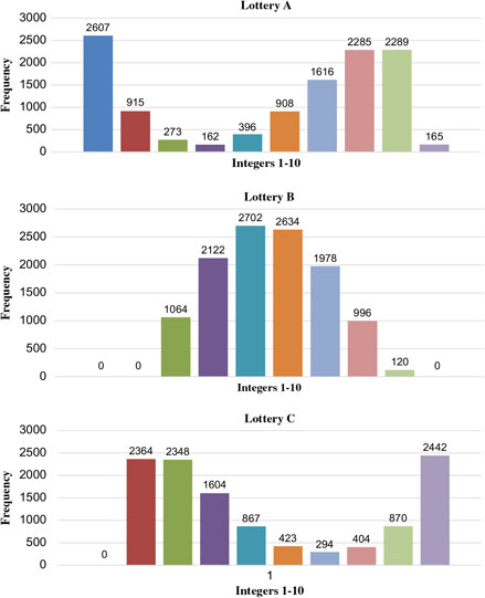
Expanding the integer range to 1–10, the distribution of integers for each of the three objects for the 3872 STP sets is shown in Figure 2. To identify these triples we first needed to generate a program for Matlab as (1) only tells us how many intransitive triples there are, not what they are. It is apparent that the PR-type pattern observed in Table 2 sharpens as the integer range expands. The reason for this goes back to the minimum of 5-levels for our original example. Lottery A comprises
${1 \over 3}$
of the worst and
${2 \over 3}$
of the second best. Lottery B has all of the middle ranks. Lottery C has
${1 \over 3}$
of the best and
${2 \over 3}$
of the second worst. This underlying structure for the three lotteries becomes smoother as the range of integers increases. By comparison, the equivalent PR structure for the $-bet is
${1 \over 3}$
of the best and
${2 \over 3}$
of the worst, and the P-bet is
${2 \over 3}$
. of the second best and
${1 \over 3}$
of the second worst.
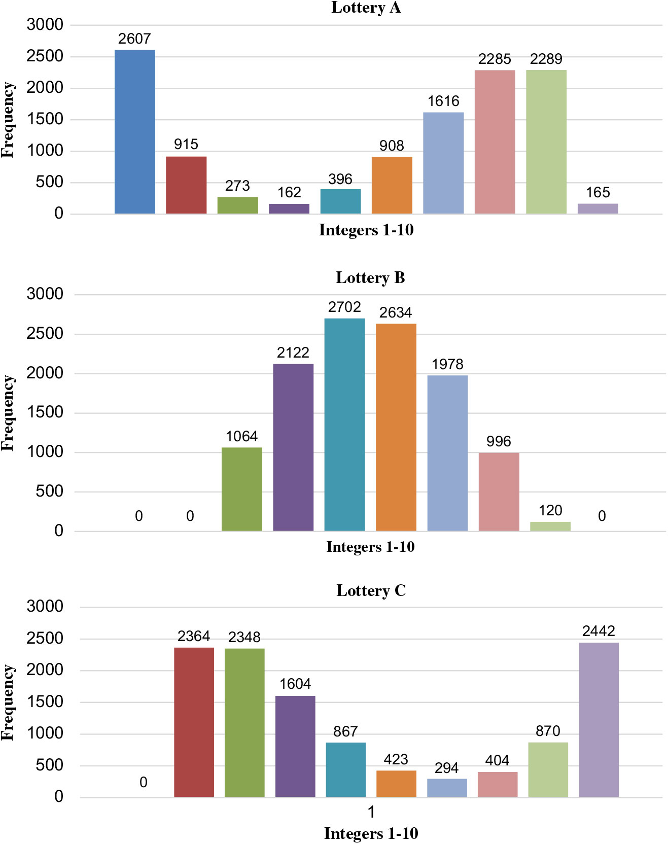
Figure 2. Distributions of integers (range 1–10) for 3872 intransitive triples.
For integer range 1–10, we can inspect the 3872 STP sets to calculate the greatest proportionate difference in expected value (EV) between the lotteries in any set. Figure 3 shows the distribution of these differences which also reveals that 92% differ less than ± 15% from the mean. Indeed, fewer than 2% of these triples differ more than ± 20%, and among any three such lotteries, the greatest proportionate difference occurs for a triple which has an EV of
 $\pound 4{2 \over 3} \pm \pound 1{2 \over 3}$
or ± 35.7%. This suggests that for preferences over lotteries, a context-independent, transitive preference ranking will result for any lottery parameters, even if an extremely non-linear comparative choice rule is used, if the objects are more distinct in EV than this. Naturally, many real world pairwise decisions are likely to have utilities which are sufficiently close that the STP will have descriptive relevance. For instance, if a choice set contains many alternatives and a decision maker uses a two-stage approach by eliminating first all obviously inferior alternatives (cf. Luce Reference Luce1959), then the reduced choice set in the second stage is likely to contain a few alternatives that are similar to each other in expected value. We might then expect intransitivity to be a distinct possibility in the second stage.
$\pound 4{2 \over 3} \pm \pound 1{2 \over 3}$
or ± 35.7%. This suggests that for preferences over lotteries, a context-independent, transitive preference ranking will result for any lottery parameters, even if an extremely non-linear comparative choice rule is used, if the objects are more distinct in EV than this. Naturally, many real world pairwise decisions are likely to have utilities which are sufficiently close that the STP will have descriptive relevance. For instance, if a choice set contains many alternatives and a decision maker uses a two-stage approach by eliminating first all obviously inferior alternatives (cf. Luce Reference Luce1959), then the reduced choice set in the second stage is likely to contain a few alternatives that are similar to each other in expected value. We might then expect intransitivity to be a distinct possibility in the second stage.
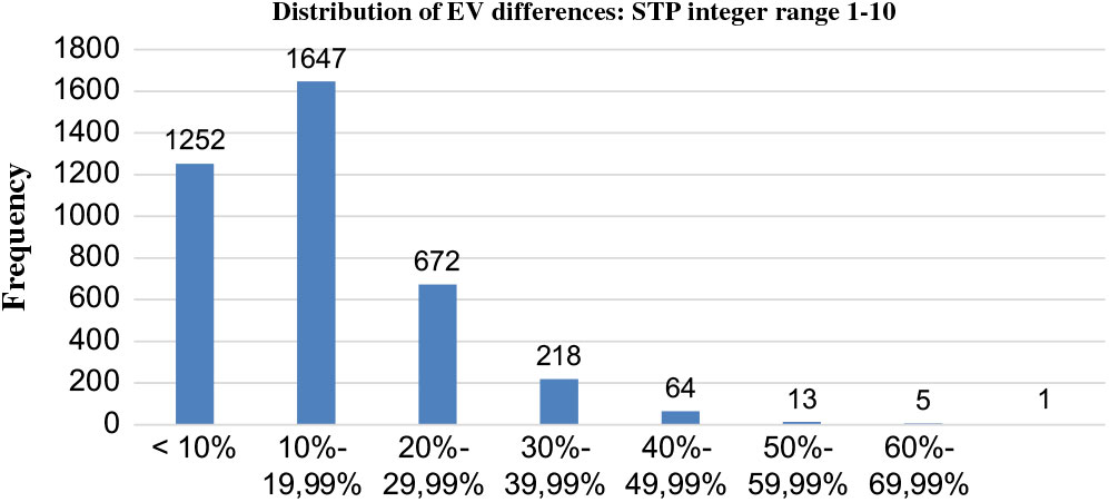
Figure 3. Distribution of max EV differences within intransitive triples.
Suppose next we consider sets comprised of more than three lotteries, where each lottery has more than three consequences. A larger proportion of cycles occurs for such sets; but these increasingly complex sets and objects are of diminishing interest to decision theorists. Suffice to note that the maximum smallest margin of victory in any paired comparison yielding a cycle increases with the number of choice objects from
 ${{\sqrt 5 - 1} \over 2}$
(i.e. 61.8%) to an asymptotic maximum of
${{\sqrt 5 - 1} \over 2}$
(i.e. 61.8%) to an asymptotic maximum of
 ${3 \over 4}$
if a choice set has a very large number of many-attribute lotteries (e.g. Usiskin Reference Usiskin1964).
${3 \over 4}$
if a choice set has a very large number of many-attribute lotteries (e.g. Usiskin Reference Usiskin1964).
We can now clarify the relative frequency of the occurrence of the ST paradox with that of the Condorcet paradox. The likelihood for the voting paradox with 3 voters and 3 alternatives is
 ${{12} \over {216}} = {1 \over {18}}$
, or 5.55% (cf. De Meyer and Plott Reference De Meyer and Plott1970). The majority of social preference orderings will not exhibit the voting paradox. Condorcet needs voters to have preference orderings that are very different from each other for the aggregation paradox to bite, which is why the frequency of a cycle at
${{12} \over {216}} = {1 \over {18}}$
, or 5.55% (cf. De Meyer and Plott Reference De Meyer and Plott1970). The majority of social preference orderings will not exhibit the voting paradox. Condorcet needs voters to have preference orderings that are very different from each other for the aggregation paradox to bite, which is why the frequency of a cycle at
 ${1 \over {18}}$
may seem low. Recall that the max-min winning probability in a binary comparison for the 3×3 STP is 61.8%, whereas in Condorcet the equivalent figure is 66.67%, so the latter paradox has greater latitude to arise than the STP.
${1 \over {18}}$
may seem low. Recall that the max-min winning probability in a binary comparison for the 3×3 STP is 61.8%, whereas in Condorcet the equivalent figure is 66.67%, so the latter paradox has greater latitude to arise than the STP.
The STP would share Condorcet’s frequency of
${1 \over {18}}$
if the three lottery’s consequences were contingent on the same states of the world and were thus jointly, not independently, distributed variables. Given statistical independence, the STP frequency is
 ${1 \over {56}}$
, or a little less than one-third as likely as its Condorcet equivalent, offering support to Kavka’s (Reference Kavka1991: 145) intuition for the frequency of the individual aggregation paradox.
${1 \over {56}}$
, or a little less than one-third as likely as its Condorcet equivalent, offering support to Kavka’s (Reference Kavka1991: 145) intuition for the frequency of the individual aggregation paradox.
In summary, our results show that the ST paradox occurs with a relatively low frequency (up to
${1 \over {56}}$
or 1.8% of all possible triples), though we note this is not too dissimilar from other influential paradoxes. The paradox emerges when three risky lotteries are reasonably close in expected value, one lottery is positively skewed, one lottery is negatively skewed and the remaining lottery is nearly degenerate (i.e. it yields one outcome nearly always). Given this clearly identifiable set of decision problems where the STP is descriptively relevant, we address next normative objections to intransitive preferences in general, of which the ST paradox is one example.
3. Objections to intransitive preferences
What are the roadblocks to the ST paradox gaining general acceptance and even facilitating breakthroughs in decision theory? We address two classes of related misunderstandings in the sub-sections below, in the hope that general acceptance of this paradox by social scientists can catalyse research that would otherwise be seen as irrational and so not pursued.
3.1. Decidability, expansion/contraction consistency and the money pump
3.1.1 Decidability
Rubinstein and Segal (Reference Rubinstein and Segal2012: 2484), using a similar STP example to ours, conclude that individuals with cyclical preferences over the binary subsets of a ternary set face an indecisiveness trap:
The indecisiveness argument is used to justify the transitivity assumption in decision theory. Suppose that A≻B, B≻C and C≻A. If the decision maker has to choose from the set {A, B, C} he will be frozen: for each alternative he may choose, he will find a better one.
Applying their claim to our original example, it is correct for a DM who selects one portfolio from {A, B, C} if she anticipates another person selecting one of the remaining two portfolios. However this decidability critique is not a decisive argument for transitivity if the chooser can identify the maximal element in the ternary set. To do so for {A, B, C} she would need to compare all three portfolios together; basic arithmetic reveals that in {A, B, C}, A will win
 ${4 \over 9}$
(when $4m occurs for A and $5m does not occur for C), B wins
${4 \over 9}$
(when $4m occurs for A and $5m does not occur for C), B wins
 ${2 \over 9}$
(when $1m occurs in A and $2m occurs in C) and C wins
${2 \over 9}$
(when $1m occurs in A and $2m occurs in C) and C wins
 ${3 \over 9}$
(whenever $5m occurs).
${3 \over 9}$
(whenever $5m occurs).
So, every person with a preference for the probable winner, including the DM in our fund manager’s example, should reveal A≻C≻B if asked to rank portfolios in the ternary choice set. However, this decidability means the preferred ranking of elements in the ternary choice set can differ from that implied by the preferred elements of the component binary sets.
3.1.2 Expansion and contraction consistency
If our ranking of lotteries in a set changes for any of its subsets, our decision would violate contraction consistency. Analogously, we would violate expansion consistency if our pairwise preference ranking reverses when it is embedded within a larger choice set. Contraction and expansion consistency together constitute transitivity’s corollary of ‘Independence of Irrelevant Alternatives’ (IIA).Footnote 9
The traditional examples used to show the attraction of IIA involve three (riskless) menu choices, e.g. chicken, beef and fish. Given the choice set {chicken, beef}, if chicken ≻ beef, then adding fish into the mix must lead either to a choice of the chicken or a choice of the fish. IIA says it is irrational to switch to the beef in the new ternary choice set {chicken, beef, fish}. IIA seems intuitively obvious for these (and many other) riskless objects, but does this analogy extend also to our earlier STP example of the ternary choice set {A, B, C}?
Notice a key implication of the decidability we established above: in the binary set {A, C} she revealed C ≻A; but with the addition of B to {A, C} in the ternary set {A, B, C}, she reveals her preference ordering is A≻C≻B. Given either ‘probable winner’ preferences or an incentive to win, she will reverse her pairwise preference ordering of A and C when these two portfolios are subsumed into the ternary set. Her reversal violates IIA even though both her binary and ternary rankings are her best decisions, in their respective choice sets, to achieve her goals.
This example demonstrates a fallacy of decomposition at a normative and most fundamental level: we cannot always use the preference ranking in the ternary set to predict choices in the component binary subsets, nor impose transitivity on revealed preferences over binary sets to predict the ternary preference ordering. Common descriptive examples of a fallacy of decomposition include the asymmetric dominance effect: adding an alternative that is dominated by one available choice option but not the other increases the chances that the dominant alternative is chosen (e.g. Huber et al. Reference Huber, Payne and Puto1982; Herne Reference Herne1999; Dhar and Simonson Reference Dhar and Simonson2003) and the attraction effect: adding an alternative that is nearly dominated by one available choice option but not the other increases the chances that the nearly dominant alternative is chosen (e.g. Huber and Puto Reference Huber and Puto1983; Simonson and Tversky Reference Simonson and Tversky1992; Tversky and Simonson Reference Tversky and Simonson1993).Footnote 10 Realizing that binary preferences do not always cohere with ternary preferences can help us to address next the famous ‘money pump’ critique of intransitive choices.
3.1.3 The money pump
If a series of pairwise comparative evaluations of choices were to end with the selection of a Pareto inferior outcome, many would argue the choice rule responsible would be one to avoid.Footnote 11 The best known such criticism of intransitive preferences is the famous ‘money pump’ originally presented by Davidson et al. (Reference Davidson, McKinsey and Suppes1955), based on an example suggested to them by Dr Norman Dalkey from the Rand Corporation (Davidson et al. Reference Davidson, McKinsey and Suppes1955: 146, fn 4).
Suppose your preference order as revealed from two binary comparisons is C≻A≻B but where B≻C for the third comparison. The money pump argument presents the following scenario. Assume you are endowed with B while I have A and C, and ɛ represents the smallest coin. I offer you A in exchange for (B + ɛ) and you accept; I then offer C for A on the same terms; again, you accept; then I offer B for C on the same terms; you accept once again. Your endowment is now (B − 3ɛ) which is dominated by the B you began with. Nor does it stop here; you will face this sequence of offers repeatedly until you are left holding B but the rest of your wealth is gone.
Several authors have put forward counterarguments to the money pump (Anand Reference Anand1987; Loomes and Sugden Reference Loomes and Sugden1987; Cubitt and Sugden Reference Cubitt and Sugden2001). The essence of their claims is that to operate a money pump profitably would require the decision maker to have neither memory of previous trades nor expectations of future trades in the money pump. In this scenario, a decision maker (DM) with neither memory nor foresight can be pumped to bankruptcy, but is such a circumscribed agent capable of rational choice at all? An unscrupulous casino could likely make money by offering a money pump game along these lines, though it would need a steady stream of novice players to make much money. This is because a less circumscribed DM will decline all trades after one cycle due to their perceiving a retrospective (and prospective) ternary choice set for the three alternatives.
Anand (Reference Anand1993a: 342; Reference Anand1993b: 62) argues that a binary preference for A over B could be viewed as a counterfactual proposition; if the DM were endowed with B and were offered A in exchange for B and a small commission fee ∊ then the DM would accept such a swap. The money pump argument is a dynamic choice problem that involves a sequence of binary choice sets {A, B}, {B, C} and {A, C}. Yet, the aggregation of three antecedent conditions of the individual counterfactual propositions does not necessarily result in the aggregate consequent of these counterfactuals (cf. Anand Reference Anand1993a: 343; Reference Anand1993b: 64).
Earlier replies left open which of the three objects the DM would, or should, choose and hold after one round of the money pump. We can take this extra step by explaining how to identify the maximal element in the ternary set. We have seen that a preference ordering from a ternary set is just as decidable as a binary preference and that contraction and expansion consistency need not always hold between binary and ternary sets. After one round of a money pump, a DM who has memory of previous exchanges must recognize the fact that a sequence of binary choice sets {A,B}, {B,C} and {A,C} exposes him or her to the union of these binary choice sets, which is a ternary set {A,B,C}. Thus, the DM should rationally choose the maximal element in the ternary set {A,B,C} which de facto originates from a sequence of binary choice sets {A,B}, {B,C} and {A,C}. At this realization, she should continue to exchange only until she is in possession once again of her preferred element from the ternary set. At this point, no further exchanges can improve her position.
Using our opening example to illustrate, she will refuse further trades once she is in possession of portfolio A. She may lose at most 2∊, with probability
${1 \over 3}$
, if she needs two trades to return to her top preference from the ternary set. This tiny penalty is a consequence of her incomplete information at the outset of the pump. But as the money pump has an expected value of just 1∊ it cannot lead to bankruptcy. As Fishburn (Reference Fishburn1991) observes: ‘it is a clever device, but one that applies transitive thinking to an intransitive world’.
3.2. On goals, primitives, reasonable rules
3.2.1 Goals and primitives
Some researchers who see the fund manager scenario of our original example accept that her pairwise preferences are rational but go on to deny that the choice sequence is intransitive. Although our example draws on the only one of 7,770 possible triplesFootnote 12 to be intransitive using the definition of Luce and Raiffa, the criteria these researchers use would suggest there is no important distinction between this triple of lotteries and the other 7,769 triples. So what is the definition of an intransitive cycle for these researchers, if it is not the one stated so clearly by Luce and Raiffa?
Their argument is perhaps best exemplified by Baron (Reference Baron2008: 247) which we interpret along the following lines. Transitivity must be understood in terms of the DM’s goals and ‘utility theory is a way of deriving choices from our beliefs and our utilities (which reflect our goals)’. In our example if the goal is to obtain the greater reward, the DM rationally selects the portfolio which maximizes that probability. If this probability is maximized by choosing A over B, then B over C, then C over A, this sequence is consistent with the rational pursuit of a fixed goal. In the above sequence, notice that the second time any portfolio is made available, it is paired with a different portfolio than in its first appearance, which means it is no longer the same portfolio with respect to its likelihood of achieving the reward.
Up to this point we are in agreement with Baron, but his argument then proceeds as follows. He claims transitivity should not be applied to these portfolios if the choice-set within which each portfolio is embedded, is changing. Re-specifying the primitives on which transitivity is defined, such that each of our preferences is conditioned on the choice set it is presented in, means instead of {A, B, C} we would now write {A|B, B|A, B|C, C|B, A|C, C|A} where x|y is a lottery that pays out if x beats y. If so, we find that {A|B ≻ B|A}; {B|C ≻ C|B}; {C|A ≻ A|C}. This move eliminates intransitivity from the preference order,Footnote 13 as |y is not the same on both occasions A is offered; but Anand (Reference Anand1993a, Reference Anand1993b) develops clear arguments against this rearguard re-specification of the choice primitives. In particular, Chapter 7 of Anand (Reference Anand1993b: 103–107) presents a series of arguments that show why, without constraints on which choices are admissible as primitives, all intransitive behaviour can be redescribed as transitive, and all transitive behaviour can be redescribed as intransitive.
The re-specification tactic can remove intransitivity only at a major cost, the consequences of which its advocates should recognize. First, in weakening transitivity to be choice-set dependent, we strip the axiom of its normative power to predict choices across choice sets. Second, it assumes the von Neumann and Morgenstern (vNM) axioms permit this switch from the assumption that ‘consequences’ are the objects of choice, to ‘consequences’ are choice-set dependent objects of choice. As far as we can tell, no explanation of how this interpretation is consistent with the vNM axiom system has yet been offered (see Sugden (Reference Sugden1996) for a related claim). Third, it loses its capacity, in combination with the other axioms, to establish the existence of any utility representation for preferences. For the purposes of economists at least, this defence needs to sacrifice the transitivity axiom in order to save it.
Interestingly, the above defence has appeal to philosophers, who like Baron, view transitivity as a property applied only to choices from fixed choice sets. From their perspective, Luce and Raiffa’s definition is ‘super-transitive’ because it applies across choice sets (e.g. Handfield Reference Handfield2016). For an economist, it is Luce and Raiffa’s definition that is transitive and the philosopher’s re-specification is one we might label ‘sub-transitive’. We agree with Anand (Reference Anand1990), who argues that if we use Baron’s and the philosophers’ interpretation, transitivity would become more a feature of language than of behaviour. This argument, however, is not specific only to the transitivity axiom; it is equally applicable to other axioms such as the independence axiom of expected utility theory.
3.2.2 An unreasonable choice rule?
It may be insightful to begin this sub-section with another famous paradox: The Prisoner’s Dilemma. This paradox was introduced to the world in a seminar by Tucker in 1950, based on a payoff matrix developed first by Flood and Dresher at the Rand Corporation, earlier that same year (Flood Reference Flood1952). They saw that for this ranking of consequences, pursuing one’s best response, dominant strategy, choice leads to an equilibrium that is Pareto inferior for both players than would be their outcomes from the non-equilibrium, dominated choice. Several years after Tucker’s description of the game, Luce and Raiffa (Reference Luce and Raiffa1957: 96–97) wrote: ‘The hopelessness that one feels in such a game as this cannot be overcome by a play on the words “rational” and “irrational”; it is inherent in the situation. There should be a law against such games!’ Should the STP be added to decision theorist’s list of banned constellations of consequences?
Today we accept the prisoner’s dilemma at face value, without rejecting the logic of choosing the best reply, even though Pareto inferior outcomes can result. Although just
 ${1 \over {78}}$
of possible unique orderings of 2×2 payoffs (up to relabelling of strategies and players) produces this paradox of rationality, its unique configuration of consequences has since set the agenda for a far deeper understanding of the tension between individual and collective interests in human society. Should we then conclude that choosing a ‘best reply’ or even a ‘dominant strategy’ is a bad decision rule and not use it? If not, why then reject probable winner preferences because of the possibility of intransitivity? In both cases it is better to simply be cognizant where and when rules such as dominance, best replies or transitivity can lead to Pareto inferior outcomes.
${1 \over {78}}$
of possible unique orderings of 2×2 payoffs (up to relabelling of strategies and players) produces this paradox of rationality, its unique configuration of consequences has since set the agenda for a far deeper understanding of the tension between individual and collective interests in human society. Should we then conclude that choosing a ‘best reply’ or even a ‘dominant strategy’ is a bad decision rule and not use it? If not, why then reject probable winner preferences because of the possibility of intransitivity? In both cases it is better to simply be cognizant where and when rules such as dominance, best replies or transitivity can lead to Pareto inferior outcomes.
Business may employ incentives such as those in our fund manager example and individuals may make pairwise comparisons for simplicity, blissfully unaware of the potentially inferior outcomes that lie in wait if they proceed to rely on transitivity for their final rankings. Indeed, Saari (Reference Saari1995) concludes ‘one must expect that many of the mathematical paradoxes from the decision and statistical sciences have been manifested by groups unknowingly selecting inferior alternatives’, a claim we argue should be extended also to individuals.
4. Conclusion: paradox regained?
Most triples of lotteries differ sufficiently in expected value that all decision takers, with either context independent (transitive) or context dependent (potentially intransitive) preferences will choose consistently with transitivity. Yet analogously to Condorcet, we have shown that for a small fraction of triples of multi-attribute choice objects evaluated in binary and ternary choice sets, rational decision makers will choose intransitively; moreover individuals who rely on the logic of transitivity will make Pareto-inferior choices from among those alternatives.
It would be a misunderstanding of the implications of the STP to argue for core utility functions without transitivity, such as Fishburn’s Skew-Symmetric Bilinear utility (Reference Fishburn1982) or Blavatskyy’s Probable Winner utility (Reference Blavatskyy2006). To see why, we need to take a step back and ask how we make choices under risk. A decision maker first looks to choose any available alternative that yields a clearly greater, context independent, expected utility. Transitivity must hold if a value attaches to each option without reference to other available alternatives (choice-set independence).
But often, no such option is apparent, so she must then proceed to compare the attributes of the available options to identify where her preference lies.Footnote 14 This cognitive effort is required to avoid welfare losses from arbitrary choice; a growing body of evidence shows preferences are often known imperfectly (inter alia, Butler and Loomes Reference Butler and Loomes2007, Reference Butler and Loomes2011). Eye-tracking experiments provide clear empirical evidence against choice-set independence when expected utilities are sufficiently ‘close’ to prompt a DM to compare the attributes of the alternatives (Russo and Dosher Reference Russo and Dosher1983; Arieli et al. Reference Arieli, Ben-Ami and Rubinstein2009; Noguchi and Stewart Reference Noguchi and Stewart2014).
A context-independent value can still result from comparing and contrasting the attributes of the available choice options. But such a process will produce an equivalent value only if utility is sufficiently ‘linear in the differences’ between the options’ attribute values; see Tversky (Reference Tversky1969); Fishburn (Reference Fishburn1982) or Loomes and Sugden (Reference Loomes and Sugden1982) for details. The STP is created from an extremely non-linear additive-difference choice rule, for which a larger difference in an attribute’s magnitude carries no extra weight. Cycles can still occur even if larger differences receive more weight than smaller differences when comparing alternatives, albeit with reduced frequency; see Butler and Pogrebna (Reference Butler and Pogrebna2018) for some examples.
To summarize, our choices will often bear the stamp of the unchosen options in their respective choice sets (Noguchi and Stewart Reference Noguchi and Stewart2014). Nor are context-dependent preferences easily dismissed as resulting from flawed decision-making heuristics which we can or should avoid. Louie et al. (Reference Louie, Haw and Glimcher2013) show how the value representations in the brain that guide our decisions take a relative, not absolute, form. Indeed, Louie et al. (Reference Louie, Glimcher and Webb2015) conclude ‘context-dependent choice behaviour may be intrinsic to biological decision-making mechanisms’ and even claim ‘context-dependent value coding may reflect an adaptive response to the intrinsic constraints of computing with biological circuitry’ (Louie et al. Reference Louie, Glimcher and Webb2015: 91).
In a world where choice alternatives are compared vis-à-vis other available alternatives, a decision process selected as most suited to human survival across deep time, we have shown that these relative evaluations, such as the likelihood that one random variable yields a better outcome than another random variable, can and sometimes should lead to intransitive revealed preferences. Yet, such intransitive preferences become ‘irrational’ when we abstract our valuations and subsequent decisions away from the context of any particular choice set. We argue that it is the latter process of stripping options from their context that is in need of justification, rather than the former. Within the context of choice sets (which differ across decision problems) such intransitive preferences can be normative, as in the STP, as well as descriptive.
Although any utility theory is supposed to represent preferences over all sets of lotteries, the existence of small, compact, locations in parameter space from which bespoke lottery pairs may create intransitive preferences, while satisfying transitivity for all others, is a challenge to all utility theories.Footnote 15 The STP demonstrates that transitivity cannot be imposed on an unrestricted domain of preference profiles to define rational choice under risk.
Rather than modelling individuals as possessing one core utility function (transitive or intransitive), typically ‘transitive’ individuals should be ‘intransitive’ in the circumstances we identify and ‘transitive’ outside of them. As this is a key lesson of the STP, it would be futile to propose a new general functional form for utility which is exclusively transitive or intransitive. Stewart et al. (Reference Stewart, Reimers and Harris2015) reach a similar conclusion: ‘The shape of the revealed utility…function is, at least in part, a property of the question set and not the individual.’ To fully account for the STP a new approach to preference representation for individual choice under risk is needed.
Acknowledgements
We thank in particular Ganna Pogrebna for her contributions to this paper. We also thank seminar participants at numerous departments and conferences for comments on earlier versions of this manuscript.
Financial support
David Butler acknowledges the support of the Australian Research Council (grant: DP1095681).
David Butler is a Professor of Economics at Griffith University, Queensland. He obtained both his Bachelor’s and Master’s degrees in economics at the University of York, UK, and his PhD from UWA (Australia). He has previously taught at the Universities of Western Australia, Arizona and Murdoch. His research interests are in experimental economics, behavioural decision theory and behavioural game theory. Particular interests include the consequences of imprecise preferences and social preferences in experimental games. His research has been published in numerous international journals, including the American Economic Review. He is a former President of the WA branch of the Australian Economic Society.
Pavlo Blavatskyy is a Professor of Economics at Montpellier Business School. He previously worked as a Professor of Economics at Murdoch University (Australia) and as a Professor of Experimental Economics at the Institute of Public Finance of the University of Innsbruck as well as an Assistant Professor at the Institute for Empirical Research in Economics of University of Zurich. He received his PhD in economics from CERGE-EI, Charles University of Prague and an MPhil in economics from the University of Cambridge. His main research interests are decision making under risk/uncertainty, probabilistic choice and intertemporal choice.