


1. INTRODUCTION
A basic premise in modern economics is that aggregate outcomes should be explained in terms of individual choices. When applied to economic modelling, this implies that models should be built by first specifying the determinants of individual behaviour (preferences, constraints), and then characterizing aggregate outcomes generated by such models in terms of individual choice parameters.
In static, single-period, models the implementation of this requirement is straightforward. The feature of these models that makes the exercise simple is that the relationship between individual behaviour and aggregate outcomes is unidirectional: individual behaviour determines aggregate outcomes, without the possibility of aggregate outcomes influencing individual behaviour. These models are, however, not suitable for analysis of a variety of intertemporal problems that involve decision-making under uncertainty.
In dynamic models suitable for this type of analysis, the implementation of the ‘bottom-up’ modelling strategy is a non-trivial issue. In multi-period models involving uncertainty, aside from the impact of behaviour on outcomes, there is the possibility that outcomes may affect behaviour. In these models, agents’ decisions are based on their expectations regarding the future, and it is possible that expectations may be revised in face of particular realizations of outcomes. From the point of view of the model-builder whose objective is to characterize equilibrium outcomes in terms of individual choices, the problem is to decide what properties of the equilibrium process the agents in the model should be assumed to know. The endogeneity of both expectations and outcomes, however, seems to make this problem unsolvable: specification of one of the determinants of agents’ behaviour (viz., their expectations) requires the knowledge of the equilibrium outcomes, which, in turn, have to be characterized in terms of the consequences of that behaviour. How does one proceed?
A deceptively simple answer was provided by Muth (Reference Muth1961). Muth exploited the interdependence between expectations and outcomes and suggested that individual expectations should be “essentially the same as the predictions of the relevant economic theory”. In other words, the proposed way out of the impasse is to postulate that expectations and outcomes coincide. The resulting model is strong-form consistent in the sense that the model solution, which is based on a set of agents’ expectations, confirms those expectations. This assumption became known as the assumption of rational expectations (RE), and has been widely used in a variety of models.Footnote 1
It should be noted that the assumption of RE plays two roles in this setting: (i) it ensures that the model is internally consistent by relating expectations and outcomes in a particular way, and (ii) it imposes restrictions on the behaviour of agents by specifying the type of knowledge agents are assumed to possess. The knowledge requirements turn out to be very strong: agents are assumed to know no less than the equilibrium stochastic process that characterizes the outcomes generated by the model, implying that they do not make systematic mistakes in their forecasts.
A large literature on the psychology of individual decision-making suggests that individual behaviour does not conform to the dictums of RE.Footnote 2 This literature has identified a variety of ad hoc rules in actual behaviour (extrapolation of past trends, decisions based on benchmarks, etc.), and found that decision-making based on these types of rules often leads to systematic and persistent errors. These findings have led some researchers to abandon the assumption of RE, and build models based on more plausible behavioural postulates.Footnote 3 Dispensing with RE, however, means that one gives up a simple solution to the endogeneity problem that at the same time ensures that the model is internally consistent. Furthermore, given that, as we shall see, the RE consistency criterion is not relevant to the non-RE models, the question of the relevant criterion arises as well. What criterion should be used? How is internal consistency of these models to be assessed? These are the questions we propose to answer in this paper.
We suggest that the assumption of rational beliefs (RB), based on the theory of rational beliefs introduced by Kurz (Reference Kurz1994), is a viable alternative to RE that addresses the behavioural concerns voiced by critics of RE. The key difference between RE and RB is that in the latter the assumption of complete knowledge of the equilibrium stochastic process is replaced by the assumption that agents know only a subset of its properties. By weakening the requirement of complete knowledge, RB allows for a wider variety of behavioural patterns than admitted under RE. At the same time, by assuming that agents do know a subset of the properties of the equilibrium process, RB establishes a link between expectations and outcomes, and thus ensures model consistency. It is clear, however, that the resulting consistency requirement is weaker than the one implied by RE. Consequently, it will be referred to as the weak-form consistency. Given that the requirements imposed by the RB assumption are in a sense minimal, we argue for the use of the weak-form consistency as a threshold consistency requirement that models without RE should satisfy.
To assess internal consistency of non-RE models using the proposed criterion, we introduce a test, and show how to apply it to a non-RE model in Cecchetti et al. (Reference Cecchetti, Lam and Mark2000). This exercise also provides an illustration of the difficulty of establishing explanatory credibility of the non-RE models that do not pass the minimal requirements that would ensure their internal consistency.
The presentation is organized as follows. In Section 2, we set up a conceptual framework suitable for representation of dynamic models under uncertainty and distinguish between restrictions on agents’ beliefs and model consistency conditions. We explain how the RE assumption ensures model consistency, what is involved in relaxing it, and introduce the RB assumption as an alternative to RE. In Section 3 we propose a test of model consistency based on the RB criterion, and illustrate its use by applying it to a non-RE model. The last section contains some thoughts on the implications of the results obtained.
2. MODEL CONSISTENCY AND BELIEF CONSISTENCY
In this section we set up a conceptual framework in which the issue of the relationship between agents’ expectations and outcomes can be given a more formal expression. The key concept needed is that of model consistency, by which we mean the existence of a relationship between agents’ expectations and outcomes generated by a model. As explained in the Introduction, the issue is relevant to stochastic dynamical models that feature decision-making under uncertainty.
Before proceeding, we need to be more precise about the meaning of “outcome” in such models. In models without uncertainty, an outcome is simply a point, such as equilibrium price and quantity at the intersection of demand and supply curves. In models with uncertainty, outcomes are not points but rather distributions over possible outcomes. When considered over time, these models can be viewed as stochastic dynamical systems, and the outcomes can be characterized as stochastic processes. In this setting, model consistency is the question of the relationship between agents’ expectations and the properties of stochastic processes generated by these models.
Denote the data a model-builder is interested in by (x 1, . . ., xN) ∈ X. The data to be explained can be viewed as being generated by an unknown process, represented as a stochastic dynamical system. Denote this system as R. The model-builder's objective is to propose a theory that explains R. The theory takes form of a model, M, consisting of i (types of) agents, i = 1, . . ., I. M can be used to generate realizations of variables of interest. Explanatory power of the model is established by comparing realizations of M to the available data generated by the true data-generating process R.
Constructing the model M involves specifying the behaviour of agents and the rules of interaction. Assumptions related to the behaviour of agents will determine what agents know, how they understand the problem, etc. This information is summarized by assuming that agents have their own models of R, which will be denoted by Mi, for each agent i. A theory, M, is a collection of models of agents’ behaviour and rules of interaction; M ≡ ((M 1, . . ., MI), φ), where φ is a proxy for interactions.Footnote 4
In representing R, Mi, and M as stochastic dynamical systems the following notation is used: X is the space of observables; Θ ≡ X ∞; (Θ, B (Θ), P) represents the probability space, where B (Θ) is a set of subsets of Θ, and P is the probability measure; (Θ, B(Θ), P, T) denotes the stochastic dynamical system, where T is the shift transformation.
We can now define the following concepts:
– True data-generating process,
where Π is the true probability measure associated with the observables.
– Model-builder's theory,
where Πm is the probability measure that characterizes the equilibrium dynamics of M.Footnote 5– Subjective models (agent i's model of the data-generating process),
where Qi represents the subjective probability measure. We also refer to Qi as the subjective belief of agent i.
To illustrate, consider a simple setting where the observables (x 1, . . ., xn) are drawn from a fixed distribution, independently over time. In that case, Π is the fixed true joint probability measure from which the data is drawn; Πm is the joint probability measure of these variables implied by the model; Qi is the joint probability measure, representing agent i's belief. More complex situations incorporating time- and distribution-heterogeneity can be accommodated within this setting in a straightforward manner.Footnote 6
Model consistency
Since M is a collection of individual models, M i, stochastic properties of M will depend on the stochastic properties of the models used by the agents.
The model M will be said to be internally consistent if there exists a mapping f (·) such that
Model consistency is the question of the existence of a mapping that establishes a relationship between agents’ beliefs and the outcomes generated by the model M.
To illustrate, consider the following example. Suppose that each of the I agents in the model decides on their demand today based on their belief about the price tomorrow. We will furthermore assume that their belief takes a simple form: each agent i believes that the prices tomorrow will be drawn from a normal distribution, with mean μi and variance σ2i. If, for simplicity, we focus on a two-period problem, each agent's belief, Q i, will take a simple form of N (μi, σ2i). Agents’ beliefs and preferences will determine the nature of their individual demand functions. We label agents’ demand functions by d i (Q i) to highlight their dependence on individual beliefs. Market demand, D, is a sum of individual demands, and its stochastic properties will depend on the properties of individual beliefs: D ≡ D(Q 1, . . ., Q I). Assuming for simplicity that the supply is constant over time, the equilibrium price will be a random variable whose stochastic properties, summarized by Πm, will be related to the stochastic properties of individual demands. The nature of the relationship between agents’ beliefs and the outcomes generated by the model will be summarized by the mapping f.
To demonstrate that a model is consistent, one has to prove the existence of f. In general, a precise characterization would be desirable as well. However, even in examples as simple as the one above, the nature of the relationship between individual beliefs and outcomes can be very complex, and a general characterization is a non-trivial exercise. Yet, without some further information regarding the nature of f, the above definition is not operational.
The way to proceed is based on the insight that underlies Muth's reasoning: rather than trying to establish general properties of f, one can impose restrictions on individual beliefs that relate these beliefs to outcomes. Since model consistency is the issue of the relationship between expectations and outcomes, by imposing restrictions on beliefs relative to outcomes, we can ensure model consistency in a direct way, and indirectly get additional information about f in particular circumstances. Consequently, we next introduce the notion of belief consistency.
Belief consistency
Belief consistency refers to the restrictions on agents’ beliefs relative to the outcomes generated by the model. An agent's belief is restricted by Πm, if there exists a mapping g(·) such that
This condition will be referred to as the belief consistency condition. Intuitively, this condition allows for a selection of a subset of properties of Q i and Πm according to the selection criterion g(·),Footnote 7 and requires that both measures coincide with respect to that subset.Footnote 8
Note that (2) is written in terms of the probability measure associated with M, rather than the true data-generating process R. This means that agents’ behaviour is evaluated relative to the belief of the model-builder. Under the admittedly strong assumption that Πm = Π, the restriction would be in terms of the properties of the true data-generating process, i.e. the process associated with the system R.Footnote 9 From the point of view of assessing the beliefs of agents in the model, however, the pertinent measure is Πm.
We now give the forms of (1) and (2) for some specific cases.
2.1 Rational expectations
Under the assumption of RE,
This corresponds to Muth's (Reference Muth1961) statement that agents’ expectations are “essentially the same as the predictions of the relevant economic theory”, where the ‘relevant economic theory’ is that of the model-builder. Beliefs consistency condition (2) holds trivially in this case, for any selection function g. Since Q i and Πm are assumed to coincide, all of their properties will coincide, regardless of which subset of properties is selected by g.
By combining (3) and the model consistency condition (1), we get
The models with RE are strong-form consistent, since there is coincidence of agents’ beliefs and outcomes along all dimensions.
To illustrate, consider an example in Lucas (Reference Lucas1978), where a representative agent has to choose optimal consumption and portfolio holdings in an uncertain environment when his endowments fluctuate randomly. The agent's decision depends on the equilibrium prices expected to prevail in the future. Conditional on his beliefs about the prices tomorrow, the agent solves his optimization problem. Given the agent's decisions, the market-clearing conditions determine the equilibrium price.
“We close the system with the assumption of rational expectations: the market clearing price function p implied by consumer behavior is assumed to be the same as the price function on which consumer decisions are based.”Footnote 10
In our terminology, the stochastic properties of equilibrium price implied by the model, summarized by Πm are the same as the stochastic properties of prices assumed by the agent in solving his optimization problem: Q i = Πm.
2.2 Irrational agents
Relaxing the assumption of RE, means that
at least for some agents. Agents whose beliefs do not coincide with Πm are said to be irrational.
It is clear that all non-RE models will be inconsistent if judged against the RE. This is particularly apparent in the context of the representative agent models.Footnote 11 To see this, consider first the model-consistency condition under RE. In a representative agent RE model, the condition (4) becomes
which implies that f must be an identity mapping. Thus, in a representative agent model with RE, coincidence of expectations and outcomes trivially ensures model consistency, which is reduced to a tautological requirement Q ≡ Πm. With an irrational agent, however, the RE model consistency condition cannot be used, since it directly contradicts the condition (5). Irrationality requires that Q ≠ Πm, while the RE model consistency criterion requires that Q = Πm.
Lucas’ reasoning can be used here as well. In that model, agent irrationality would imply that the market-clearing price implied by the agent's behaviour is not the same as the price function on which the agent's decisions are based. Equivalently the stochastic properties of equilibrium price implied by the model, summarized by IIm are not the same as the stochastic properties of prices assumed by the agent in solving his optimization problem.
The use of the RE-based model consistency condition may be inappropriate for non-RE models, but it is not obvious a priori what criterion to use to assess consistency of these models. Alternatively, how does one solve the endogeneity problem described in the Introduction, while relaxing the assumption that expectations and outcomes coincide?
2.3 Rational beliefs
The answer to these questions starts from the observation that the condition (5) does not preclude the possibility that g(Q i) = g(Πm), for some selection function g. In other words, even though agents’ beliefs and the equilibrium probability measure are not identical, it is still possible that they coincide on a subset of properties. This opens up the possibility of arriving at a notion of model consistency based on a coincidence on a subset of properties of expectations and outcomes. The key issue becomes to decide on what that subset should be. A priori, there seem to be many possibilities. Here, we describe one option, based on the theory of rational beliefs, introduced by Kurz (Reference Kurz1994).
The theory of rational beliefs relaxes the assumption that beliefs and outcomes coincide, so that the starting point, given by (5), is the same as in any non-RE model. But, rather than taking this to imply that g(Q i) ≠ g(Πm), it explicitly specifies a subset of properties on which expectations and outcomes are required to coincide. This subset is used to restrict the types of beliefs agents are allowed to hold, and to ensure model consistency.
The RB restrictions are closely related to a particular primitive assumption that underlies the theory of rational beliefs. The theory is built on the premise that agents operate in non-stationary but stable environments. Intuitively, a non-stationarity environment is an environment which, at the extreme, does not display any regularities that can form a (statistical) basis for knowledge. At the other end of the spectrum is the assumption of stationarity which can be interpreted to mean that the environment displays a particularly strong set of regularities, which can form a basis for knowledge.Footnote 12
The assumption of stability is best understood as imposing restrictions on the extent of non-stationarity. A stable environment is an environment which, while non-stationary nonetheless displays some regularities that can form a basis for knowledge.Footnote 13 The implications of stability are two-fold:
– It precludes the possibility of complete knowledge. Partial knowledge in the theory of RB is not a consequence of agents’ optimizing behaviour in which the costs of acquisition of complete knowledge exceed the expected benefits, but a consequence of non-stationarity of the environment.
– It provides the restriction on agents’ beliefs. The assumption of stability implies the existence of a stationary distribution function associated with a stochastic dynamical system. The use of this distribution to restrict agents’ beliefs is the key to ensuring model consistency.
Denote the stationary distribution associated with agents’ models (M i) by m Qi, for each agent i, and the stationary distribution associated with the model (M) by m Πm. Let g be the selection criterion such that g(Q i) = m Qi for all agents i, and g(Πm) = m Πm. Under the theory of rational beliefs, the belief consistency condition (2) takes the form
Drawing on Lucas’ reasoning again, (6) states that the subset of properties of the stochastic process characterizing the behaviour of equilibrium price in the model, given by m Πm, coincides with the same subset of properties of the stochastic properties of prices assumed by the agent in solving his optimization problem, mQi.
The key differences between (3) and (6) are that the latter permits diversity of agents’ beliefs and allows for a much wider range of behaviour of individual agents than is permitted under RE. The cost of introducing diversity is that in these environments strong-form consistency has to be replaced by the consistency criterion
The condition (7) is clearly weaker than the condition (4), since it posits the existence of a relationship using only a subset of properties of the equilibrium probability measure Πm.Footnote 14
3 A TEST OF MODEL CONSISTENCY WITH AN EXAMPLE
3.1 The test
Suppose we are given a model in which the assumption of RE has been replaced by an ad hoc behavioural postulate. We would like to know whether this model satisfies the minimal requirements of the weak-form consistency given by (7). The proposed test relies on the comparison of mQi and m Πm, the stationary distributions associated with individual models, M i, and the aggregate model M.Footnote 15 The test is based on the observation that the stationary distribution functions determine the behaviour of the long-run moments in the model. Therefore, if the model is consistent, the long-run moments computed under mQi and m Πm will coincide. The test is performed in two steps:Footnote 16
(i) Compute the equilibrium price mapping in the model, given the selection of beliefs of agents.
(ii) Simulate the economy either under the probability measure Πm or under the subjective beliefs of any agent. Under the rationality of beliefs assumption both procedures should yield the same long-term empirical moments of all observed variables. Should this turn out not to be the case, we conclude that the model is not weak-form consistent.
3.2 An example
The equity premium puzzle, originally identified by Mehra and Prescott (Reference Mehra and Prescott1985), refers to the inability of a particular type of asset pricing model to explain the difference in observed returns on bonds and equity (Kotcherlakota, Reference Kocherlakota1996). In a recent attempt to explain the puzzle, Cecchetti et al. (Reference Cecchetti, Lam and Mark2000)Footnote 17 relax the assumption of RE in Mehra and Prescott's model and replace it by the assumption that the representative agent is persistently irrational. Keeping the other features of the original model intact, CLM demonstrate that, for a judicious choice of parameters, their model can explain the puzzle. Given that this is a non-RE model, the question is whether it is weak-form consistent. To verify this, we perform the test described in Section 3.1. The reader is referred to Misina (Reference Misina2006) for a detailed investigation of the implications of the findings of this paper.
3.2.1 A brief description of the model
The data that the model-builder is interested in explaining consists of historical returns on stocks and bonds, and, more specifically, their observed differences. The data are assumed to have been generated by some underlying process R = (Θ, B(Θ), Π, T). The model-builder proposes a theory M to explain R. The standard model, used by Mehra and Prescott (Reference Mehra and Prescott1985) as well as by CLM is a model of an exchange economy in which there are two assets-stocks and bonds. The model has, in effect, only one agent, whose actions are determined by a specification of preferences, endowments, and agent's expectations. These three ingredients yield the subjective model, M i used by the agent. There are, by construction, no interactions in the model.
Stochastic properties of equilibrium prices and returns in this model will depend on agent's beliefs about the process underlying the endowment uncertainty. The model is built on the assumption that at any given time, endowments can take one of the two possible values – high or low – which is selected randomly. The probability of getting endowments in each state is ![]() . The true relationship between endowments today and tomorrow is given by the transition matrix, Γ. Elements of this matrix are πij – probabilities of being in state j tomorrow if the current state is i.
. The true relationship between endowments today and tomorrow is given by the transition matrix, Γ. Elements of this matrix are πij – probabilities of being in state j tomorrow if the current state is i.
CLM assume that, rather than using Γ, the representative agent uses a different matrix, ![]() , and solves his optimization problem. Given the agent's decision, the market-clearing conditions determine the equilibrium prices and returns. The equity premium, ep, implied by the model is then computed as the difference in returns on stocks and bonds.
, and solves his optimization problem. Given the agent's decision, the market-clearing conditions determine the equilibrium prices and returns. The equity premium, ep, implied by the model is then computed as the difference in returns on stocks and bonds.
Since there are two exogenously specified transition matrices, Γ and ![]() in this model, there are four possible ways to obtain equilibrium price and returns:
in this model, there are four possible ways to obtain equilibrium price and returns:
a. using Γ to compute equilibrium prices and returns,
b. using
to compute equilibrium prices and returns,c. using
to compute equilibrium prices and F to compute returns, andd. using Γ to compute equilibrium price and f to compute returns.
Whereas the multiplicity of ways to do the computations may be unsettling, this will in general be the case in non-RE models, including the RB models. The RB assumption will, however, imply that the long-run statistics will be identical in all these cases. To test whether the CLM model satisfies the minimal requirements of weak-form consistency, we compute and compare the long-run statistics under Γ and ![]() .
.
3.2.2 Results
Table 1 contains the results for this model. Rows 2–5 of the table correspond to different specifications of the parameter values (risk-aversion, subjective discount rate, etc.), which, according to the authors solve the puzzle.Footnote 18 For each set of specifications of parameter values (Cases 1 to 4), we have computed prices and expected returns using the methods a.–d. The numbers in the table are the equity premia generated by the model. For example, epa corresponds to the equity premium when Γ is used to compute both equilibrium prices and returns in the model.
Table 1. Results of the weak-form consistency test.
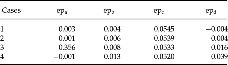
Given that the parameter values in a given case are the same, the values of ep for that case should be identical if the model is weak-form consistent, regardless of which method of computation is used. For example, model consistency would imply that for Case 1, epa = epb = epc = epd. The same would hold for cases 2, 3, and 4 as well.
As is clear from Table 1, the long-run statistics generated by this model under different computations are vastly different: the equality epa = epb = epc = epd does not hold in any of the cases considered. We therefore conclude that the CLM model is not weak-form consistent.
We are now presented with a puzzle: Which one of these four different sets of results should be taken as representative? CLM report the third case, epc, and claim explanatory success. Sceptics need only point to the other three sets of results and claim explanatory failure. Although one could argue that this is the symptom of a lack of consensus on the criterion for selecting results, it is more plausibly viewed as a symptom of an internally inconsistent model whose explanatory credibility is questionable.
4 CONCLUDING REMARKS
The assumption of rational expectations (RE) plays two roles in economic models: it imposes restrictions on behaviour of agents, and it ensures model consistency. Dissatisfaction with RE on behavioural grounds has led some researchers to replace it by more behaviourally plausible postulates. However, in these undertakings the issue of model consistency seems to have been ignored, with potentially serious implications for explanatory credibility of the resulting models.
In this paper we introduced a conceptual framework that facilitates the analysis of this issue, and pointed to potential problems that the abandonment of RE entails. The key difficulty is that in non-RE models, the strong-form consistency associated with the RE models is inapplicable. The challenge is to propose an alternative consistency condition that would at the same time address the concerns of the critics of RE.
We proposed the theory of rational beliefs as an alternative that fulfills both tasks: it ensures model consistency while addressing the concerns associated with learning and behavioural implications voiced by critics of RE. The weak-form consistency implied by the RB condition is in a sense a minimal requirement. Whether it is satisfied in a given model can be tested using the method described in this paper.
The rationality of beliefs assumption and the test proposed in this paper can be used in two ways. First, if the model builder decides to impose the RB condition a priori, the model will be consistent and there is no need for further demonstration. Second, if beliefs are not restricted a priori and RB is used as the relevant beliefs consistency condition, the test can be used to establish whether a given set of beliefs satisfies this condition. Positive evidence would constitute a demonstration that the model used is consistent.
Are there other ways of ensuring model consistency? Once the concept of model consistency is extended to include weaker-form consistency conditions, and once one starts thinking about the relationship between expectations and outcomes in terms of restrictions of the former on a subset of the latter, the set of possibilities becomes rather large. Within the general framework of this paper the issue becomes a matter of choice of a particular subset of properties of outcomes that would be used to restrict agents’ beliefs. Theory of rational beliefs uses a particular subset, and one might argue that, given the weak nature of requirements implied by RB, any alternative would likely contain RB as a special case, but the question is an open one, and an interesting avenue for further exploration.
The key message of this work is that to relax the assumption of RE is not simply a matter of replacing it by an ad hoc behavioural postulate, but rather a matter of arriving at an alternative equilibrium concept, which addresses the issue of interdependence of expectations and outcomes, and deals with the problem of model consistency. We urge great caution in using non-RE models in which these issues are not explicitly addressed, and suggest the use of the test in this paper to determine whether such models satisfy at least the minimal consistency conditions implied by RB. In light of the explanatory problems with inconsistent models illustrated in Section 3.2, we propose that any aspiring non-RE model be considered inconsistent until proven otherwise.
The above findings may result in a rather pessimistic assessment of the overall prospects. Given, on the one hand the evidence against RE, and, on the other hand, a rather dubious status of models without it, why not simply reject the latter and accept the idea that humans are intrinsically irrational and that explanations of such behaviour that rely on rationality are simply not feasible? We believe that such pessimism would be premature. First, this paper gives at least one alternative to RE that allows for behaviour which from the RE perspective would be judged irrational, but still does not yield “anything goes” results. Second, the message of behavioural psychologists is that “though this be madness, yet there is method in it.” Whereas researchers in the area have identified a number of deviations from rational behaviour, there is a pattern to these deviations.Footnote 19 Systematic and persistent deviations could be indicative of an inappropriate criterion used to judge rationality as much as the behavioural problem itself.

