1. INTRODUCTION
The strong consistency of least squares estimators in a vector
autoregression with deterministic terms is studied. Autoregressions
generally have three types of asymptotic behavior in that they may be
stationary, a random walk type process, or an explosive process. For the
econometric analysis of nonexplosive time series it usually suffices to
use weak consistency and weak convergence arguments as in the work by
Phillips (1991) and Johansen (1995). When a time series has explosive features it is
mathematically more natural to use strong consistency arguments exploiting
that explosive processes tend to follow persistent trajectories with
probability one.
The first results showing consistency for explosive first-order
autoregressions were due to Rubin (1950) and
Anderson (1959), with some generalizations by,
for instance, Fuller, Hasza, and Goebel (1981)
and Jeganathan (1988). A general strong
consistency result for vector autoregressions was given by Lai and Wei
(1985), and this is generalized here to a
situation with deterministic terms as seen in econometric models. The
techniques employed are to a large extent based on methods presented by
Lai and Wei (1982, 1983a, 1983b, 1985) and Wei (1992).
The paper is organized so that Section 2 presents the model and an
overview of the main results. The proofs follow in Section 3–10 and
will be outlined in Section 2.
The following notation is used throughout the paper. For a matrix
α let α[otimes ]2 = αα′, whereas α
[otimes ] β is the Kronecker product and equals for example
(α11 β,α12 β) if α ∈
R1×2. Further
diag(α1,…,αn) is a block
diagonal matrix with diagonal blocks αj. When
α is symmetric then λmin(α) and
λmax(α) are the smallest and the largest eigenvalue,
respectively. The choice of norm is the spectral norm ∥α∥ =
[λmax(α[otimes ]2)]1/2,
implying that ∥α−1∥ =
[λmin(α[otimes ]2)]−1/2.
Whereas
is a conditional expectation, the notation
(Yt|Zt)
denotes the residual of the least squares regression of
Yt on Zt. The
abbreviation a.s. is used for properties holding almost
surely.
2. THE AUTOREGRESSIVE MODEL AND MAIN
RESULTS
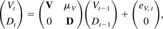
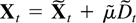
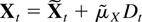
The model in this paper is for a p-dimensional time series,
X1−k,…,X0,…,XT
satisfying a kth-order vector autoregressive equation
where Dt−1 is a deterministic term
and εt an innovation term.
The innovations are required to satisfy the local
Marcinkiewicz–Zygmund conditions for convergence of explosive
processes introduced by Lai and Wei (1983a).
These are that (εt) is a martingale difference
sequence with respect to an increasing sequence of σ-fields
with the properties that some conditional moments of higher order are
bounded and that the conditional variance has positive definite limit
points.
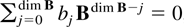
Each of the Assumptions 2.1 and 2.2 excludes the possibility that the
innovations could be autoregressive conditional heteroskedastic (ARCH) as
proposed by Engle (1982). Therefore these
conditions would probably be perceived as too strong for nonexplosive
situations, but for general autoregressions they are convenient.
The deterministic term Dt is a vector of
terms such as a constant, a linear trend, or periodic functions such as
seasonal dummies. Inspired by Johansen (2000)
the deterministic terms are required to satisfy the difference
equation
where D has characteristic roots on the complex unit circle.
For example
will generate a constant and a dummy for a biannual frequency. The
deterministic term Dt is assumed to have
linearly independent coordinates, which is formalized as follows.
Assumption 2.3. |eigen(D)| = 1 and
rank(D1,…,Ddim D)
= dim D.
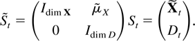
With this type of deterministic term the time series can be written
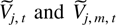
conveniently in companion form. The stacked process
Xt−1 =
(Xt−1′,…,Xt−k′)′
satisfies
when defining matrices B and μ and a process
eX,t as
whereas St =
(Xt′,Dt′)′,
which combines Xt with the deterministic
process Dt, satisfies
where S and eS,t are
defined as
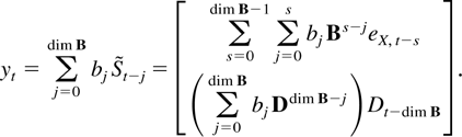
The main object of interest is the least squares estimator for the
parameters
A1,…,Ak,μ,
which has the form
where St−1[otimes ]2 is
the outer product St−1
St−1′. The partial estimator for
the dynamic parameters
A1,…,Ak can
correspondingly be written in terms of the residuals
(Xt|Dt)
from regressing the companion vector Xt on
the deterministic terms Dt as
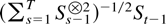
whereas the least squares variance estimator satisfies
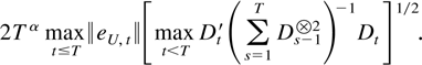
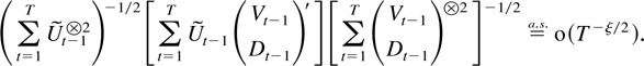
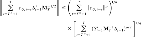
The first main result gives a bound for a studentized version of the
joint estimator.
THEOREM 2.4. Suppose Assumptions 2.1–2.3 are
satisfied. Then
The remainder term can be decomposed as a sum of the following
terms:
Special cases have been proved by Pötscher (1989, Lemma A.1) for dim D = 0 and ξ = 0
and by Nielsen (2001a), who proves a univariate
version holding in probability.
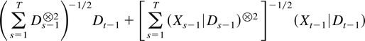
The proof of Theorem 2.4 relies on a separation of the stochastic and
deterministic components using that
can be rewritten as
by partitioned inversion. For the least squares estimator itself a
more complete understanding of the interaction between the deterministic
components and unit root processes appearing in the denominator matrix is
needed. Such results are not available as yet, and the following
consistency results are therefore only partial although they do represent
some improvement over previous results and include a complete description
of the pure stationary and purely explosive cases where
|eigen(B)| ≠ 1.
THEOREM 2.5. Suppose Assumptions 2.1–2.3 are
satisfied. Then
If B and D have no common
eigenvalues then
The issue of consistency of the least squares estimator was first
discussed for a univariate, explosive, Gaussian first-order
autoregression, with dim X = 1, dim D = 0, by Rubin
(1950) and Anderson (1959). Lai and Wei (1985,
Theorem 4) studied strong consistency for the special case without
deterministic terms, so dim D = 0, and gave a weaker result with
ξ = 0. A related generalization has previously been presented by
Duflo, Senoussi, and Touati (1991, Theorem 1) in
the case where the explosive roots have multiplicity one, whereas their
Theorem 2 seems false in suggesting that the least square estimator for
B otherwise is inconsistent.
A direct consequence of Theorem 2.4 concerning the studentized least
squares estimator is that the least squares variance estimator can be
estimated consistently.
COROLLARY 2.6: Suppose Assumptions 2.1–2.3 are satisfied.
Then
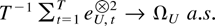
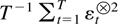
Although Assumptions 2.1 and 2.2 suffice to ensure that the sequence
is relatively compact with positive definite limit points as argued by
Lai and Wei (1985), some further structure is
needed to get convergence to an interpretable matrix. In light of
Assumptions 2.1 and 2.2 it is convenient to apply the following sufficient
condition used by Chan and Wei (1988).
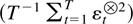
Assumption 2.7.
where Ω is positive definite.
This gives rise to the following convergence result.
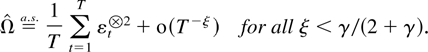
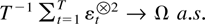
THEOREM 2.8. Suppose Assumptions 2.1 and 2.7 are satisfied.
Then
Corollary 2.6 and Theorem 2.8 lead to an immediate result for the
least squares variance estimator.
COROLLARY 2.9. Suppose Assumptions 2.1, 2.3, and 2.7 are
satisfied. Then
There is potential for many other econometric applications of Theorem
2.4. An example is lag length determination, where it is conceptually
important to establish the lag length before determining the location of
the characteristic roots; see Pötscher (1989), Wei (1992), and
Nielsen (2001b). Other examples are unit root
testing (Nielsen 2001a) and cointegration
analysis (Nielsen, 2000), where the asymptotic
inference results also can be used without knowledge about the
characteristic roots.
The remainder of the paper gives the proofs of these results. To a
large extent the proofs follow those of Lai and Wei (1983b and 1985) but with
many modifications because of the deterministic term. The proofs are
outlined as follows. In Section 3 the process
Xt is decomposed into autoregressive
components
Ut,Vt,Wt
with characteristic roots outside, on, and inside the unit circle,
respectively. The order of magnitude of the deterministic process,
Dt, and the process itself,
Xt, is discussed in Sections 4 and 5,
respectively. The next sections are concerned with the order of magnitude
of the denominator matrix
.
As a first step the sample correlation of Ut
and Dt is considered in Section 6. The order
of magnitude of the largest and the smallest eigenvalue of
MT is then discussed in Sections 7 and 8,
respectively. The next step is to discuss sample correlations of all
possible combinations of the processes
Ut,Vt,Wt,Dt
in Section 9, and finally the main results are proved in Section 10.
3. DECOMPOSITIONS OF THE PROCESS
The process Xt is decomposed in two ways
to facilitate the subsequent asymptotic analysis. The first decomposition
concerns the stochastic part of the process whereas the second
decomposition disentangles deterministic and stochastic parts of the
process.
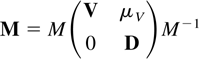
The first decomposition separates the eigenvalues of the companion
matrix B for the stochastic part of the process. Following
Herstein (1975, p. 308) there exists a regular,
real matrix M that transforms B into a real block
diagonal matrix with blocks U, V, and W having
eigenvalues with absolute value less than one, equal to one, and larger
than one, respectively. That is,
For the purpose of proving the results of Section 2 it can be assumed
without loss of generality that B =
diag(U,V,W) is block diagonal and
St =
(Ut′,Vt′,Wt′,Dt′)′.
The second decomposition seeks to separate the stochastic and
deterministic components and is based on two arguments. The processes
Ut,Wt,Dt
are first separated by a similarity transformation using that the matrices
U, W, and D have no common eigenvalues, whereas
the processes
Vt,Dt have to be
discussed in more detail because the matrices V and D
may in general have common eigenvalues.
The processes
Ut,Wt are linear
functions of the deterministic process Dt,
and they are first shown to satisfy the relationships
with
.
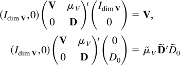
The argument is the same in both cases. Taking
Ut as an example consider the companion
matrix for the vector
(Ut′,Dt′)
and apply a similarity transformation of the form
The result (3.1) then follows by arguing that
can be chosen so
.
Because the matrices U and D have no common eigenvalues
a unique solution
can be found according to Gantmacher (2000, p.
225).
In the special case where B has no eigenvalues in common with
D the same argument can be made for the entire process
Xt as for the
Ut,Wt processes.
That is,
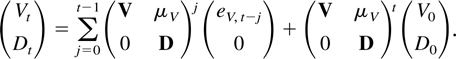
When it comes to the general situation where V and D
are allowed to have common eigenvalues it is convenient first to discuss
the special case where V and D have their eigenvalues at
one and are both Jordan matrices
with (Λ,E) = (1,1). In that situation
Vt will be shown to satisfy
with
and where
is of the form (3.4) with
.
To see this write the process
(Vt,Dt) in
companion form as
which has the solution
The result (3.5) is therefore a consequence of the following two
properties:
for some matrices
.
The second property is proved as follows. Because V and
D are both Jordan blocks of the form (3.4) with eigenvalues at
one a real matrix M exists so that
is a block diagonal matrix with diagonal elements that are Jordan
blocks of the form (3.4) with (Λ,E) = (1,1). The left-hand
side of (3.7) can then be written as a sum:
for some matrices
μj,Dj,0 and Jordan
blocks Dj. Writing the vector
Dj,0 as T(0,1)′ where
T is an upper triangular band matrix and noting that upper
triangular band matrices commute then
μjDjtDj,0
=
μjDjtT(0,1)′
=
μjTDjt(0,1)′.
This in turn can be written as
,
ensuring the desired result (3.7) with
.
In general V and D can have eigenvalues anywhere on
the unit circle. Suppose these occur at l distinct complex pairs
exp(iθj) and
exp(−iθj) for 0 ≤
θj ≤ π, which of course reduce to a single
eigenvalue of 1 or −1 if θj equals 0 or
π. Following Herstein (1975, p. 308) and
using Assumption 2.3 to D there exist regular, real similarity
transformations MV and
MD that block-diagonalize V and
D as
where the subblocks Vj,m and
Dj are real Jordan matrices of the form (3.4)
and where (Λ,E) is one of the pairs
Using the same argument as before it therefore holds in general that
Vt has representation (3.5) where
has subcomponents
of dimension dim Vj and dim
Vj,m, respectively, and
has subcomponents
of dimension
.
Combining the results (3.1), (3.2), and (3.5) with the notation
shows that the process without loss of generality can be represented
as
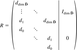
It is convenient also to introduce the dimensions
and also the maxima
4. LIMITING RESULTS FOR THE DETERMINISTIC
COMPONENT
In the following discussion the order of magnitude of the
deterministic process Dt and the denominator
matrix
will be described.
The main result is formulated using normalization matrices
THEOREM 4.1. Suppose Assumption 2.3 is satisfied. Then it
holds that
Two lemmas concerning the order of
are needed.
LEMMA 4.2. Let Dj,1,0 denote the last
element of the initial vector Dj,0.
Then
where f is the polynomial vector f(n + 1,u)
=
[un/(n!),…,u0/(0!)]′.
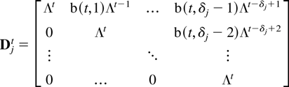
Proof of Lemma 4.2. The process
Dj,t satisfies
Dj,t =
DjtDj,0
where
and b(·,·) is the binomial coefficient. The desired
result then follows by noting that
uniformly in t whereas ∥Λn∥ ≤
∥Λ∥n = 1. █
LEMMA 4.3.
Proof of Lemma 4.3. (i) By Lemma 4.2 the cross-product satisfies
Trigonometric identities show that
ΛjtDj,1,0
Dj,1,0′(Λjt)′
equals
Ej∥Dj,1,0∥2/dim
Λj + Rj where
Rj = 0 for dim Λj = 1
and Rj = cos(2θt)A +
sin(2θt)B for some constant matrices
A,B when dim Λj = 2. When dim
Λj = 1 the desired result follows immediately,
whereas when dim Λj = 2 it follows from the
result
for any constant a; see Gradshteyn and Ryzhik (1965, 2.633.2).
(ii) Note that the vector f (n,u) can be
expressed as a nonsingular linear transformation of the first n
Legendre polynomials, p(n,u), say, which have
the property that
giving the positive definiteness.
(iii) Use the same type of arguments as in (i), noting that
ΛjtDj,1,0
Dm,1,0′(Λmt)′
equals cos(2θt)A + sin(2θt)B
for some constant matrices A,B. █
(i)The result follows from Lemma 4.2 by stacking the
processes Nδj
Dj,t and using the triangle
inequality.
(ii) Lemma 4.3 implies that
converges to a block diagonal matrix with positive definite diagonal
elements.
(iii) The desired result follows from (i) and (ii) and
replacing each Dt with
ND Dt.
█
5. THE ORDER OF MAGNITUDE OF THE
PROCESS
In the following discussion the order of magnitude of the process
Xt is investigated. This is a generalization
of Lai and Wei (1985, Theorem 1) where the case
without deterministic components is considered. Subsequently a convergence
result is given for the explosive component
Wt.
To describe the order of magnitude of Xt
let λj denote the distinct eigenvalues of
B whereas mj is the multiplicity of
λj. Define the multiplicity of the largest
eigenvalue as
The following result then holds.
THEOREM 5.1. Suppose Assumptions 2.1 and 2.3 are satisfied. Then,
for ξ < γ/(2 + γ),
Proof of Theorem 5.1. By (3.9) it holds that
.
Lai and Wei (1985, Theorem 1) show the results
for the purely stochastic component
,
whereas the order of the deterministic component
follows from Lemma 4.2. █
When studying the process
Lai and Wei (1985) use the following
generalization of the Marcinkiewicz–Zygmund theorem.
THEOREM 5.2 (Lai and Wei, 1983a, Corollaries
3 and 4). Suppose Assumptions 2.1 and 2.2 are satisfied. Then for any
sequence of matrices At the series
converges a.s. if and only if the series
converges. If this holds, and At ≠ 0
for infinitely many t, then
for any variable Y that is
-measurable for some t.
This result yields a more precise statement about the order of
magnitude of the explosive component.
COROLLARY 5.3. Suppose Assumptions 2.1–2.3 are satisfied.
Then
Proof of Corollary 5.3.
6. CORRELATION BETWEEN STATIONARY AND
DETERMINISTIC COMPONENTS
One major difference between the results presented here and the work
of Lai and Wei (1985) is that deterministic
terms are included in the model. Before turning to the question of how big
the denominator matrix can be in Section 7 it is convenient to consider
the asymptotic order of magnitude of correlations between the zero mean
process with roots smaller than one,
,
and the deterministic component, Dt.
As a first step toward discussing the sample correlation of
,
results of Lai and Wei concerning the matrices
are stated. The results give conditions for relative compactness of
sequences of such matrices. Recalling that the relative compactness of a
sequence is the property that the limit points fall in a compact set, this
enables a discussion of the order of magnitude of the sequence under weak
assumptions. In particular, a condition is given ensuring that the limit
points are bounded away from zero.
THEOREM 6.1 (Lai and Wei, 1985, Theorem 2,
equation (3.7), Example 3). Suppose Assumption 2.1 is satisfied. Then,
with probability one, the matrix sequences
are relatively compact with the same limit points.
If in addition Assumption 2.2 is satisfied, the limit points are
positive definite.
Because eU,t is a linear
combination of εt the sequence
is therefore relatively compact. In addition the following results can be
shown.
THEOREM 6.2 (Lai and Wei, 1985, Theorem 2,
Example 3). Suppose Assumptions 2.1 and 2.2 are satisfied. Then it
holds with probability one that
and also it holds that
Before turning to the sample correlation of
it is useful to cite the following univariate result by Wei (1985).
LEMMA 6.3 (Wei 1985, Lemma 2). Suppose
Assumption 2.1 is satisfied. Let (xt)
be a sequence of random variables adapted to
with
.
Assume
for some η > 0. Then
The result for the sample correlation of
can now be stated and proved.
THEOREM 6.4. Suppose Assumptions 2.1–2.3 are satisfied.
Then, for all η > 0,
Proof of Theorem 6.4. Theorem 6.2 shows that
,
so it suffices to show that
.
The main contribution arises from the sum
for an α satisfying 1 > α > 0. With this in mind and using
the object of interest can be written as
The first two terms in (6.1) are o(Tη). To
see this bound their norm by
and use Theorems 4.1 and 5.1 and that
∥U∥Tα decreases
exponentially.
The third term in (6.1) is o(Tη). To see this
use Dt =
DsDt−s
and the normalization ND given in (4.1) to
rewrite it as
The norm of this expression is bounded by
Because the sum
converges it suffices to show that the last two components can be
approximated uniformly by a variable that is
o(Tη).
The sum
is approximately equal to
,
which converges to a positive definite matrix; see Theorem 4.1. The norm
of the approximation error,
,
is bounded by
,
because of Theorem 4.1.
In a similar way
is approximately
,
which is not dependent on s. Considering each element of this
matrix and applying Lemma 6.3 shows that this is
o(TηND−1).
The approximation error can be bounded by
Using Theorems 4.1 and 5.1 this is seen to be
o(Tα−ξ/2), which is o(1) for a small
α. █
Some immediate consequences of these results are the following
examples.
Example 6.5
Suppose Assumptions 2.1 and 2.7 are satisfied. Then Theorems 6.1 and
6.2 imply
and in particular
for some matrix ΩU, so
Example 6.6
Suppose Assumptions 2.1–2.3 are satisfied. Then Theorems 6.2 and
6.4 and equation (3.1) imply that the sequence of matrices
is relatively compact with positive definite limit points. Moreover,
this series converges almost surely if
is convergent. According to Example 6.5 this is for instance the case if,
in addition, Assumption 2.7 is satisfied.
7. THE LARGEST EIGENVALUE OF THE DENOMINATOR
MATRIX
The order of magnitude of the largest eigenvalue of the denominator
matrix
can now be described. This is followed by a convergence result for the
purely explosive case and a bound for the rate of convergence of sum of
powers of
.
First, the largest eigenvalue of MT is
considered in the following generalization of Lai and Wei (1985, Corollary 1).
THEOREM 7.1. Suppose Assumptions 2.1–2.3 are satisfied.
Then
Proof of Theorem 7.1. If max|eigen(B)| < 1
then
by (3.1). Lai and Wei (1985, Corollary 1) show
and the result then follows from Theorems 4.1 and 6.4. If
max|eigen(B)| ≥ 1 the result follows directly
from Theorem 5.1. █
For the explosive part of the process the following generalization of
Lai and Wei (1985, Corollary 2) can be
established.
COROLLARY 7.2. Suppose Assumptions 2.1–2.3 are satisfied
and min|eigen(B)| > 1 so
and recall the definition of W in Corollary 5.3. Then
where FW is positive
definite a.s.; hence
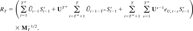
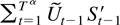
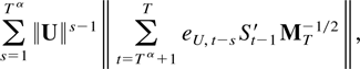
Proof of Corollary 7.2. Let RT denote the
difference between the matrices
.
The decomposition (3.2) shows
which vanishes for large T because of Theorem 4.1(i) and
Corollary 5.3(i). The desired result is then a direct consequence of Lai
and Wei (1983b, Theorem 2). █
Whereas Theorem 7.1 gives a bound for the sum of squares of the
process, the following result gives a bound for sums of higher order
powers of the stationary component.
THEOREM 7.3. Suppose Assumption 2.1 is satisfied. Then, for
all η > 0 and ζ < γ,
Proof of Theorem 7.3. For notational convenience define
.
Using Hölder's inequality it follows that
Summation over t then gives the following bound:
Changing summation index in the double sum, this can be bounded
further by
The first two sums converge, whereas the third term can be decomposed
as
The latter term is of order O(T) =
o(T1+η) by Assumption 2.1. The first term is a
martingale. Normalized by T1+η it converges to
zero a.s. on the set where
see Hall and Heyde (1980, Theorem 2.18).
Minkowski's inequality shows that this sum is finite if the sum
is finite. Assumption 2.1 ensures that this is the case. █
8. THE SMALLEST EIGENVALUE OF THE
DENOMINATOR MATRIX
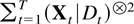
Three results are given concerning the order of the inverse of the
denominator matrix,
,
of the least square estimator in the nonexplosive case. Using the
techniques of Chan and Wei (1988) it can be
proved that T−1MT
is bounded from below in a weak convergence sense. The first result goes
some way toward an almost sure version of this result in showing that the
partial denominator matrix
is bounded from below, whereas the second result shows that the joint
matrix T−1MT is
bounded from below in the special case where B and D
have no common eigenvalues. In combination these results can be used to
establish the third result concerning the order of
maxTα≤t≤T
St′MT−1St
without actually establishing the order of
MT−1, and this will suffice
to prove the main theorems.
The first result concerns the partial denominator matrix
and is related to Lai and Wei (1985, Theorem
3).
THEOREM 8.1. Suppose Assumptions 2.1–2.3 are satisfied
and |eigen(B)| ≤ 1.
Then
To prove Theorem 8.1 the following lemma is needed. This lemma ensures
that Lai and Wei (1982, Lemma 1) concerning the
order of magnitude of normalized least squares estimators can be used.
LEMMA 8.2. Suppose Assumptions 2.1–2.3 are satisfied.
Then
Proof of Lemma 8.2. It suffices to show that
u′MTu > 0 for all
u ∈ Rdim S so u ≠ 0
and some T. Because
it is equivalent that
(S0,…,ST−1)R
spans Rdim S for some invertible matrix
R.
The decomposition (3.9) shows that
where
.
The Cayley–Hamilton theorem (see Herstein, 1975, p. 334) implies that if
with d0 = 1 is the characteristic polynomial of
then
and in particular
,
say. Define
and partition R as a (2 × 2)-block matrix so the upper
right block is a dim
-dimensional square matrix. The preceding properties then show
that
(S1,…,ST)R
is an upper triangular (2 × 2)-block matrix. The lower right block
is
,
which spans Rdim D by Assumption 2.3. It is
left to prove that the upper left block
spans Rdim X. The process
zt is a linear combination of the process
that satisfies a first-order autoregression without deterministic terms.
The desired result then follows from Lai and Wei (1985, Theorem 3) using Assumptions 2.1 and 2.2.
█
Proof of Theorem 8.1. Let m = dim X. Using the model
equation (2.3) and that
Dt−1−j =
D−1−jDt
the process Xt can be rewritten as
where eX,0 = X0,
eX,−t =
−μDt−1, and
X−t = 0 for t > 0. It
follows that
It is now argued that the lower bound in (8.1) satisfies
The norm of the difference between the left-hand side and the first
term on the right is bounded by
The first sum is finite, so when normalized by the denominator term it
is seen to be O(1) as a result of Lemma 8.2. The normalized second term is
O[(log T)1/2] as a result of Lai and Wei
(1982, Lemma 1), which can be used because of
Lemma 8.2.
Using Lai and Wei (1982, Lemma 1) once again
in combination with Theorem 6.2 shows that, for j <
k,
This in turn implies that
The proof is completed by combining (8.2), (8.3), and Theorem 6.2.
█
When B and D have no common eigenvalues Theorem 8.1
can be extended.
THEOREM 8.3. Suppose Assumptions 2.1–2.3 are satisfied
and B and D have no common
eigenvalues. Then lim infT→∞
λmin(T−1MT)
> 0 a.s.
Proof of Theorem 8.3. Because of the representation
given in (3.3) it suffices to show the result for sums of squares of
If
is the characteristic polynomial of B the Cayley–Hamilton
theorem (see Herstein, 1975, p. 334) implies
,
and hence
Because B and D have no common eigenvalues then
.
It follows that
using Theorems 4.1, 6.2, and 6.4 and Lai and Wei (1985, equation (3.19)). The argument is finished as in
the proof of Lai and Wei (1985, Theorem 3).
█
The final and more technical result addresses the order of
St′MT−1St.
Lai and Wei (1985, Lemma 4) show that
maxt≤T
St′MT−1St
vanishes when |eigen(B)| ≤ 1 and dim D
= 0. For the subsequent analysis it suffices to take a maximum over just
Tα ≤ t ≤ T for some 0 <
α < 1 requiring that 0 < |eigen(B)| but
allowing dim D > 0.
THEOREM 8.4. Suppose Assumptions 2.1–2.3 are satisfied and
that 0 < |eigen(B)| ≤ 1. Then
for all α,ζ so 0 < α < 1 and
ζ < min[γ/(2 +
γ),½].
Theorem 8.4 will be proved in a few steps following Lai and Wei (1983b). The first step is to strengthen their Lemma
3.
LEMMA 8.5. Let (at) be a
sequence of nonnegative numbers satisfying the following
conditions.
Then aT =
o(T−ρ) for all ρ <
min(1,κ/2).
Proof of Lemma 8.5. Condition (i) implies that for every 0 < ρ
< 1 it holds that
minT>t≥T−Tρ
at ≥ aT
− 2CTρ−κ for all large T.
In particular, choosing ρ to satisfy 0 < ρ <
min(1,κ/2), it is seen that
Combining this with (ii) it follows that
.
Because δ can be chosen arbitrarily small this proves the desired
result. █
The second step is to generalize Lai and Wei (1983b, Lemma 6ii).
LEMMA 8.6. Suppose Assumptions 2.1–2.3 are satisfied
and max|eigen(B)| ≤ 1. Define
T0 as in Lemma 8.2. Then
Proof of Lemma 8.6. The proof is the same as that of Lai and Wei
(1983b, Lemma 6ii) using the generalizations of
their Theorem 3 and Lemma 6i presented previously in Theorem 7.1 and Lemma
8.2. █
The third step is to generalize Lai and Wei (1983b, Lemma 7).
LEMMA 8.7. Suppose Assumptions 2.1–2.3 are satisfied and
that 0 < |eigen(B)| ≤ 1.
Then
Proof of Lemma 8.7. (i) Using Lai and Wei (1983b, Lemma 5i) in the same way as in the proof of
Lai and Wei (1983b, Lemma 7i) it holds that
where
This expression can be rewritten using the identities
for ι = (Idim X,0). The
desired result follows by noting that
according to Lai and Wei (1982, Lemma 1), which
can be used because of Lemma 8.2, whereas the term
by Theorem 8.1.
(ii) Noting that ST =
SST−1 +
eS,T it holds that
The norm of the first term is less than
by (i). This is in turn bounded by
because of Lemma 8.6(i). The second term equals
according to the identities (8.4) and is seen to be
o(T−ξ/2) by Theorems 5.1 and 8.1.
█
Theorem 8.4 can now be proved.
Proof of Theorem 8.4. Lemmas 8.6(ii) and 8.7(ii) show that the
conditions of Lemma 8.5 are satisfied for the sequence
St′Mt−1St
with κ = ζ/2 and therefore
tζ/4St′Mt+1−1St
= o(1) for large t. For t > T0
then Mt−1 >
Mt+1−1 so that
St′MT−1St
≤
St′Mt+1−1St,
and thus for all ε > 0 and almost every outcome a
T1 exists so that for all t,T so
that T > t ≥ T1 it holds that
St′MT−1St
≤
St′Mt+1−1St
< ε. This in turn implies that for all ε > 0 and almost
every outcome a T1 exists so that for all T
so that T > T1 it holds that
maxTα≤t<T
St′MT−1St
≤
St′Mt+1−1St
< ε as desired. █
9. SAMPLE CORRELATIONS
It has already been established in Section 6 that the sample
correlation of
and Dt vanishes asymptotically. In the
following discussion the remaining sample correlations of pairs of the
processes
are studied. A first result concerns the sample correlation of
Wt and
Ut,Dt.
THEOREM 9.1. Suppose Assumptions 2.1–2.3 are satisfied.
Then
The bound for the sample correlation of
should be viewed in light of the results of Anderson (1959). He found that
is convergent when the innovations εt are
independent, identically distributed, but in general divergent. The stated
result combined with Theorem 6.1 shows that the order of
YT is at most
o[T(1−ξ)/2] for martingale
difference sequence innovations.
Proof of Theorem 9.1. The norms of the two expression are bounded
by
where m is either of
The last two terms of (9.1) are convergent according to Corollaries
5.3 and 7.2. It holds that mD =
O(T−1) by Theorem 4.1, whereas
mU = o(T−ξ)
because Theorem 5.1 shows
,
whereas the denominator term is O(T−1) by
Example 6.6. █
For the sample correlation between Wt and
St=(Vt′,Dt′)′
a different type of proof is needed using the results of Section 8. This
is because the order of the smallest eigenvalue of
is unknown.
THEOREM 9.2. Suppose Assumptions 2.1–2.3 are satisfied.
Then, for all ζ < min[γ/(2 +
γ),½], it holds that
Proof of Theorem 9.2. For convenience define
Because
is convergent according to Corollary 7.2 it suffices to show that
.
Follow Anderson (1959, Theorem 2.2) in
writing
Because
it follows, for any 0 < α < 1, that
The first two terms in (9.3) vanish exponentially fast. Their norm is
less than
where
∥W∥Tα−T
vanishes exponentially, MT−1
= O(1) by Lemma 8.2, and the remaining terms are of polynomial order
according to Theorem 5.1 and Corollary 5.3.
The final term in (9.3) is o(T−ζ/8).
Its norm is less than
where the first two components converge (see Corollary 5.3) and the
last component is o(T−ζ/8) by Theorem
8.4. █
Remark 9.3. The bottleneck in the proof of Theorem 9.2 is the order of
magnitude of
maxTα<t≤T
St′MT−1St.
By extending the weak convergence results of Chan and Wei (1988) it can be proved that this term is
when |eigen(B)| ≤ 1, implying that the sample
correlation between Wt and
(Vt′,Dt′)
is
.
Wei (1992, Theorem A.1) considers the sample
correlation between Ut and
Vt in the univariate case dim X = 1
when Dt is absent and
εt is a martingale difference sequence
satisfying Assumptions 2.1 and 2.7. That result can be generalized and
strengthened by a proof resembling that of Theorem 6.4.
THEOREM 9.4. Suppose Assumptions 2.1–2.3 are satisfied.
Then, for all ξ < γ/(2 + γ),
Proof of Theorem 9.4. Define St,
S, eS,t, and
MT as in (9.2). Theorem 6.2 shows that
,
so it suffices to show that
.
Inspired by the proof of Theorem 6.4 and Wei (1992, Theorem A.1) write
for some 0 < α < 1 so that
The first term in (9.4) is
o[T(1−ξ)/2]. The norm of the
sum
is bounded by
,
which is of the desired order when α is chosen small enough and using
Theorem 5.1, whereas
MT−1/2 is bounded as a
result of the positive definiteness of MT
stated in Lemma 8.2.
The second term in (9.4) is o(1). By Cauchy–Schwarz inequality
its norm is bounded by
where ∥U∥Tα vanishes
exponentially and the other terms are O[(T log
T)1/2] as a result of Theorem 6.2 and Lemma
8.6(ii).
The third term of (9.4) is
o[T(1−ξ)/2]. Its norm is
bounded by
according to the triangle inequality. Hölder's inequality
implies
for 2 < p < 2 + γ and p−1
+ q−1 = 1. Because q/2 < 1 and
Tα > T0 for large
T, then
(St′MT−1St)q/2
≤
St′MT−1St
≤
St′Mt−1St,
so the last term is o(Tη) for all η > 0
according to Lemma 8.6(ii). Because of Theorem 7.3 then
uniformly in s. Overall the sum in t is therefore
o[T(1−ξ)/2] uniformly in
s. The desired result then follows because
converges. █
Tables 1 and 2
give an overview of the sample correlation results of Theorems 6.4, 9.1,
9.2, and 9.4. All pairs of
have been considered except for
Vt,Dt, which has
nonnegligible sample correlation when V and D have
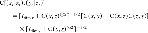
common characteristic roots. To produce these tables it is used that the
marginal sample correlation, C(x,y), of processes
xt,yt relates to
joint correlations by
according to the formula for partitioned inversion, and also by
Order of pairwise sample correlations, with η > 0 and ξ
< γ/(2 + γ)
Order of pairwise sample correlations, with η > 0 and ξ
< γ/(2 + γ)
As a consequence of the results summarized in Table
2 the condition |eigen(B)| ≤ 1 can be
eliminated in Theorem 8.1 concerning the lower bound for
.
COROLLARY 9.5. Suppose Assumptions 2.1–2.3 are satisfied.
Then
Proof of Corollary 9.5. Let Rt =
(Ut′,Vt′)′.
Using a similarity transformation M as described in Section 3 and
the results in Table 2 shows that
equals
a.s. Apply Theorem 8.1 to the upper left block and Corollary
7.2 and Theorem 9.1 to the lower left block. █
10. PROOFS OF MAIN RESULTS
The proofs of the main results in Theorems 2.4, 2.5, and 2.8 now
follow. The first of these results concerns the studentized least squares
estimator.
Proof of Theorem 2.4. The process St is a
linear combination of Rt =
(Ut′,Vt′,Dt′)′
and Wt. As a consequence of Theorems 9.1 and
9.4 the sample correlation of Rt and
Wt vanishes asymptotically; see also Table 1. The vector of interest therefore equals
so the nonexplosive and explosive components can be considered
separately.
For the explosive component note that the norm of
is bounded by
where the first two terms are convergent because of Corollaries 7.2
and 5.3. The order of the last term is given in Theorem 5.1.
For the nonexplosive part with max|eigen(B)| =
1 Lai and Wei (1982, Lemma 1) together with
Theorem 7.1 shows the desired result.
For max|eigen(B)| < 1 then Lemma 6.3
combined with Theorems 4.1, 6.2, and 6.4 shows the result. █
By combining Theorem 2.4 with results for the denominator matrix
established in Sections 7 and 8 the strong consistency result for the
least squares estimator can now be proved.
Proof of Theorem 2.5. Consider first the partial estimator.
Transforming Xt into
(Rt′,Wt′)
with Rt =
(Ut′,Vt′)′
using a similarity transformation M as described in Section 3
shows that
equals
The sample correlation between
(Rt−1|Dt)
and
(Wt−1|Dt)
vanishes asymptotically, so it suffices to prove the result for the two
special cases where max|eigen(B)| ≤ 1 so dim
W = 0 and where min|eigen(B)| > 1 so
dim R = 0. In the first case the desired order follows from
Theorems 2.4 and 8.1 whereas in the second case the statistic vanishes
exponentially fast as a result of Theorem 2.4 and Corollary 7.2.
The second result for the full estimator when B and
D have no common eigenvalues follows from Theorems 2.4 and 8.3.
█
Proof of Theorem 2.8. Assumption 2.7 shows that
mt =
a′(εt2 −
Ω)b for arbitrary dim X-vectors a and
b. Hall and Heyde (1980, Theorem 2.18)
show that if 1 ≤ p ≤ 2 then
on the set
.
This set has probability one if p ≤ 1 + γ/2 and
p(ζ − 1) < −1 according to Assumption 2.1.
These restrictions are satisfied when ζ < min[γ/(2 +
γ),½]. █