Published online by Cambridge University Press: 19 July 2005
This paper considers estimation and inference in panel vector autoregressions where (i) the individual effects are either random or fixed, (ii) the time-series properties of the model variables are unknown a priori and may feature unit roots and cointegrating relations, and (iii) the time dimension of the panel is short and its cross-sectional dimension is large. Generalized method of moments (GMM) and quasi maximum likelihood (QML) estimators are obtained and compared in terms of their asymptotic and finite-sample properties. It is shown that the asymptotic variances of the GMM estimators that are based on levels in addition to first differences of the model variables depend on the variance of the individual effects, whereas by construction the fixed effects QML estimator is not subject to this problem. Monte Carlo evidence is provided showing that the fixed effects QML estimator tends to outperform the various GMM estimators in finite sample under both normal and nonnormal errors. The paper also shows how the fixed effects QML estimator can be successfully used for unit root and cointegration tests in short panels.We are grateful to Karim Abadir, Stephen Bond, Jinyong Hahn, Marc Nerlove, Ingmar Prucha, and, especially, Manuel Arellano, Peter Schmidt, Peter Phillips (the editor), and four anonymous referees for helpful and constructive comments. We have also benefited from useful suggestions by participants at various seminars and conferences.
Over the past decade important advances have been made in the study of dynamic panel data models where both the time dimension (T) and the cross-sectional dimension (N) are large. See, for example, the surveys by Baltagi and Kao (2000) and Phillips and Moon (2000) and the references cited therein. In this paper we are concerned with the more traditional panel literature where N is large and T is short (typically 10 or less), which remains the prevalent setting for the majority of empirical microeconometric research.1
For references to much of this empirical work see, for example, Baltagi (2001).
As in single equation dynamic panel data models there are two main issues that need to be addressed in the study of PVARs. (i) The fact that T is fixed necessitates the modeling of the initial observations.2
For discussions of the initial observations in the single equation context see, for example, Anderson and Hsiao (1981, 1982), Bhargava and Sargan (1983), Blundell and Smith (1991), and Nerlove (1999).
Dealing with possible slope coefficient heterogeneity poses further complications and might not be feasible in dynamic panels where T is very short. See, for example, Hsiao, Pesaran, and Tahmiscioglu (1999).
See, for example, Anderson and Hsiao (1981) and Nickell (1981) for a discussion of this issue in the context of single equation models.
To overcome this problem generalized method of moments (GMM) estimation has been suggested in the literature. It is useful to distinguish between the “standard” GMM estimators proposed by Holtz-Eakin et al. (1988) and Arellano and Bond (1991) and their subsequent extensions by, for example, Ahn and Schmidt (1995), Arellano and Bover (1995), and Blundell and Bond (1998). The “standard” GMM estimators are based on orthogonality conditions that interact the lagged values of the endogenous variables with first differences of the model's disturbances, whereas the “extended” GMM estimators augment these orthogonality conditions with additional moment conditions implied by homoskedasticity and initialization restrictions.
This paper develops random and fixed effects QML estimators (RE-QMLE and FE-QMLE, respectively) when it is not known a priori whether the underlying series are stationary, have unit roots, or are cointegrated. It contributes to the discussion of the initialization of dynamic models with a fixed T by generalizing the stationarity restrictions proposed in the literature to settings involving unit roots and cointegration. New panel unit root and cointegration tests are proposed for panels with short T. Under certain regularity conditions it is shown that the QML estimators are consistent and asymptotically normally distributed (as N → ∞, with T fixed and short), irrespective of whether the underlying time series are (trend) stationary, integrated of order one, I(1), or I(1) and cointegrated. The paper also provides a generalization of the extended GMM estimators to PVARs and presents a comparative analysis of these estimation procedures in terms of their asymptotic properties and also their finite-sample performances using Monte Carlo experiments. The RE-QMLE is more efficient than the FE-QMLE, but it imposes moment homogeneity restrictions on the initial observations and requires the individual effects to be random draws from probability distributions with finite fourth-order moments. The standard and extended GMM estimators are also shown to impose restrictions on the distribution of the individual effects not needed under the fixed effects specification. It is shown that the asymptotic variance of the standard and extended GMM estimators conditional on the variance of the model disturbances increases as a function of the variance of the individual effects. This is an important result and shows that in dynamic panels the performance of the GMM estimators could be adversely affected, possibly substantially, when the individual effects exhibit considerable variations. By contrast, the FE-QMLE is by construction invariant to the variation of the individual effects and hence is not subject to the same problem. The importance of the variance of the individual effects for comparisons of the FE-QMLE and GMM estimators is also investigated by means of Monte Carlo experiments. It is documented that the FE-QMLE performs well under a variety of parameter configurations (including unit roots) and nonnormal errors.
The remainder of this paper is organized as follows. Section 2 introduces the PVAR model. Sections 3 and 4 develop the QML estimators under random and fixed effects specifications, respectively. Section 5 proposes new tests for unit roots and cointegration in panels with short time dimension. Section 6 discusses GMM estimation of the PVAR model. Monte Carlo simulation results regarding the finite-sample performance of the QML and GMM estimators are presented in Section 7, and Section 8 concludes and provides some suggestions for future research. The Appendix provides a proof of the dependence of the asymptotic variance of the standard GMM estimator on the variance of the individual effects.
Let wit be an m × 1 vector of random variables for the ith cross-sectional unit at time t and suppose that the wit's are generated by the following PVAR model of order one, PVAR(1):

for i = 1,2,…,N and t = 1,2,…,T, where Φ denotes an m × m matrix of slope coefficients, μi is an m × 1 vector of individual-specific effects, εit is an m × 1 vector of disturbances, and Im denotes the identity matrix of dimension m × m. For simplicity we restrict our exposition to first-order PVAR models.
We shall consider both random and fixed effects specifications of the individual-specific effects in the remainder of this paper, highlighting their differences and the implications these differences have for estimation and inference. However, for both the random and fixed effects specifications we make the following general assumptions.
Assumption (G1). The available observations are wi0,wi1,…,wiT, with T ≥ 2 but fixed as N → ∞.
Assumption (G2). The disturbances εit, t ≤ T, are independently and identically distributed (i.i.d.) for all i and t with E(εit) = 0 and Var(εit) = Ωε, Ωε being a positive definite matrix.
For panels with N and T sufficiently large and under certain conditions it is possible to relax the cross-sectional independence assumption; see, for example, Conley (1999), Phillips and Sul (2003), Bai and Ng (2004), Moon and Perron (2004), and Pesaran (2003, 2004). Exploring the issue of cross-sectional dependence in the context of the PVAR model with T fixed is beyond the scope of the present paper.
Let ξit = wit − μi and note that (2.1) can also be written as

with

When T is fixed, it is necessary to consider the initialization of the wit-process for estimation and inference. We make the following assumption.
Assumption (G3). The initial deviations, ξi0, are i.i.d. across i, with zero means and the constant nonsingular variance, E(ξi0ξi0′) = Ψξ0.
Under Assumption (G3), if all eigenvalues of Φ fall inside the unit circle, then the process (2.1) can either start from an infinite past or a finite past. If some of the eigenvalues of Φ are equal to unity, then the nonstationary direction can only start from a finite past.
The PVAR(1) model (2.1) is the generalization of the univariate dynamic panel data model considered, for example, in Ahn and Schmidt (1995) to the multivariate context,

which would be equivalent to (2.1) when all eigenvalues of Φ fall inside the unit circle. However, in the presence of unit roots the two specifications (2.1) and (2.3) will have different trend properties, with the unrestricted intercepts specification (2.3) exhibiting linear trends whereas the restricted specification (2.1) does not. In what follows we adopt (2.1) as the data generating mechanism, although for estimation purposes it is often more convenient to work with (2.3).
In this case the general assumptions, (G1)–(G3), need to be supplemented with additional assumptions on the individual-specific effects, μi. In particular, we make the following assumption.
Assumption (R1).

This is a standard assumption for the random effects model and together with the general assumptions (G1)–(G3) yields

where ai = (Im − Φ)μi,

Ωa = (Im − Φ)Ωμ(Im − Φ)′, Ω0a = Cov(wi0,ai), and Ω0 and Ωa are, respectively, positive definite and nonnegative definite matrices.5
Assumption (R1) could be relaxed, for example, to allow the individual effects μi to have a common nonzero mean. Nonzero correlations between the disturbances εit and the initial observations wi0/the individual effects μi could also be allowed for, but they will not be considered here because in general it is not possible to test whether these correlations are zero or nonzero. See Ahn and Schmidt (1995) for more detailed discussion of this in the single equation setting.
Assumption (R2). All elements of the cross-product matrices ritrit′, t = 1,2,…,T, have finite second-order moments.
Denote the [2m2 + 3m(m + 1)/2] × 1 vector of unknown coefficients by θ,

where φ = vec(Φ), σε = vech(Ωε), σa = vech(Ωa), σ0 = vech(Ω0), and σ0a = vec(Ω0a).
Assumption (R3). θ ∈ Θ, where Θ is a compact subset of

and the true parameter vector, θ0, falls in the interior of Θ.
Assumption (R1) can be derived from more primitive assumptions concerning the initialization of the wit process. For example, in the case when wit is stationary and has started in the infinite past we have6
For further details see Binder, Hsiao, and Pesaran (2004).

and

Let
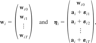
and note that ηi = Rwi, where R is a matrix of dimension m(T + 1) × m(T + 1) given by
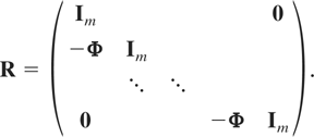
The RE-QML estimator of θ is derived by maximizing the following log-likelihood function, which assumes normally distributed errors, as the criterion function:

where7
Notice that Ση is nonsingular even if initialization restrictions such as Ωa = 0 and Ω0a = 0 that follow under Φ = Im are imposed. To allow the possibility of nonstationarity of initial observations and/or the case where the process is stationary but had not started from an infinite past, in our estimation setup Ωa and Ω0a will be treated as unrestricted coefficient matrices.

with ιT being a T × 1 vector of ones, and

We then have the following proposition.8
A proof can be established using familiar techniques as reviewed, for example, in White (1994).
PROPOSITION 3.1. Under assumptions (G1)–(G3), and (R1)–(R3), and assuming that (2.1) holds, then as N → ∞, SN,w converges almost surely to the nonstochastic matrix Σw, and the RE-QMLE of θ, defined by maximizing (3.3), is consistent. Furthermore, under these assumptions

where

with

being a positive definite matrix.
Remark 3.1. If time-specific effects are present, and wit is generated by9
The presence of N cross-sectional units allows us to consider a nonparametrically specified common trend for all cross-sectional units.

where δt is an m × 1 vector of time-specific effects, then upon redefining for estimation purposes
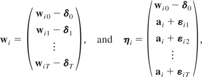
the log-likelihood function is again given by (3.3). It can be shown that the RE-QMLE of δt is given by

In the special case where δt = δt, t = 0,1,…,T, the RE-QMLE of δ can be obtained using the following weighted average of the unrestricted estimates,

:

where we have partitioned Σw−1 into (T + 1)2 blocks of dimension m × m,
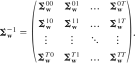
The RE-QMLE of the remaining parameters, θ, can be computed using the concentrated log-likelihood function.
Under the fixed effects specification no restrictions need to be placed on the probability distribution function generating the individual-specific effects μi in (2.1) (or, in unrestricted form, ai in (2.3)). In particular, Assumptions (R1) and (R2) are no longer required. It can then be allowed, for example, that (i) the individual effects are dependently distributed, (ii) the individual effects are heteroskedastic, (iii) the individual effects are (more generally) characterized by a joint probability distribution function with the number of unknown parameters increasing at the same rate as the number of cross-sectional observations in the panel, (iv) the individual effects do not have moments, and (v) the individual effects and the disturbances are correlated.
Following standard practice the μi's can be eliminated by first-differencing (2.1), namely,10
Hsiao, Pesaran, and Tahmiscioglu (2002) in the univariate context show that the QML estimator is invariant to the choice of the T × (T + 1) transformation matrix

that is of rank T and eliminates the individual-specific effects, namely, that has the property that

, with

being a vector of constants of dimension (T + 1) × 1. The argument in Hsiao et al. (2002) readily extends to the multivariate setting considered here.

To obtain a consistent QML estimator one needs to work with the unconditional joint probability distribution of (Δwi1,Δwi2,…,ΔwiT), or the distribution of (Δwi2,Δwi3,…,ΔwiT) conditional on Δwi1, and ensure that these distributions are free of the incidental parameters problem. The latter condition is obviously satisfied if the unconditional distribution of Δwi1 does not depend on any incidental parameters. Therefore, for the fixed effects specification we shall supplement Assumptions (G1)–(G3) with the following assumption.
Assumption (F1). The following moment restrictions are satisfied:
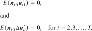
where κi0 = (Im − Φ)ξi0.
Combining this assumption with Assumptions (G1)–(G3) and using (2.2) we now have11
Assumptions (G3) and (F1) can be relaxed to allow for κi0 to have a constant nonzero mean and for Cov(κi0, εi1) and Cov(κi0,Δεit), for t = 2,3,…,T, to be nonzero and possibly time-varying (but still homogeneous across i).

where

with Ψξ0 already defined in Assumption (G3).
Remark 4.1. The first-differencing operation simultaneously deals with the incidental parameters and unit root problems. Unlike in time-series models, first-differencing in panels with T fixed still allows identification and estimation of the long-run (level) relations that are of economic interest irrespective of the unit root and cointegrating properties of the wit process.
Remark 4.2. It is important to note that Assumption (F1) imposes homogeneity restrictions on a linear combination of the initial deviations, (Im − Φ)ξi0, and the initial error terms, εi1, for all i, without imposing any such restrictions on the individual effects, μi, themselves.
The following moment and parameter space assumptions will also be needed.
Assumption (F2). The second moments of the cross-product matrix Δrit Δrit′, t = 2,3,…,T, with

exist.
Denote the [m2 + m(m + 1)] × 1 vector of unknown coefficients by ρ,

where φ = vec(Φ), σε = vech(Ωε), and ψ = vech(Ψ).
Assumption (F3). ρ ∈ Ξ, where Ξ is a compact subset of

and the true parameter vector, ρ0, lies in the interior of Ξ.
Let
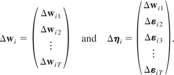
It follows that Δηi = RΔwi, where R is given by (3.2), but its dimension now is mT × mT, with

and
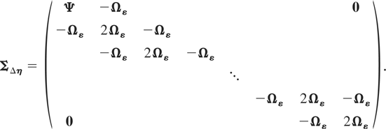
The QML estimator of ρ is obtained by maximizing the following log-likelihood function based on the joint probability distribution of (Δwi1, Δwi2,…,ΔwiT) under the normality assumption:12
The likelihood function (4.4) holds whether T is finite or approaches infinity. However, if T → ∞, one can estimate μi consistently, and hence one may apply QML estimation to (2.1) instead of working with (4.4).

where

PROPOSITION 4.1. Under assumptions (G1)–(G3), and (F1)–(F3), and assuming that (2.1) holds, then as N → ∞, SN,Δw converges almost surely to the nonstochastic matrix ΣΔw, and the FE-QMLE of ρ, defined by maximizing (4.4), is consistent. Furthermore, under these assumptions

where

with H[ell ] being a positive definite matrix.
Remark 4.3. If wit is generated by the fixed effects counterpart of (3.4), so that time-specific effects are present, we have that

with γt = Δδt. Upon redefining
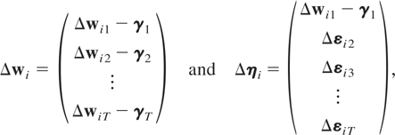
the log-likelihood function is again given by (4.4). Using similar derivations as in the random effects setting, it can be shown that the FE-QMLE of γt is given by

In the restricted case of γt = γ, t = 1,2,…,T, we have

where ΣΔw−1 is partitioned into m × m-dimensional blocks ΣΔwts, t,s = 1,2,…,T, analogous to the partition in (3.5).
Remark 4.4. Computation of the FE-QMLE is complicated by the fact that the matrix ΣΔη will often be high-dimensional. However, to compute the determinant and inverse of ΣΔη, one may make use of the block-tridiagonal structure of ΣΔη. Applying the block LDL′ factorization to ΣΔη, the latter may be factorized as

, where

is a block-diagonal matrix with jth diagonal block given by

, and where

, with

being a block-subdiagonal matrix with all subdiagonal blocks equal to Ωε.
13For further details see, for example, Binder and Pesaran (2000), who in the context of the solution of multivariate linear rational expectations models discuss the block LDU factorization, of which the block LDL′ factorization is a special case.

To compute the inverse of ΣΔη, a computationally efficient scheme is to adapt the recursions based on Bowden's procedure in Binder and Pesaran (2000), which yields

and

where ΣΔη,jl−1 denotes the jlth block of ΣΔη−1, j,l = 1,2,…,T. Further details of our numerical algorithm that renders computation of the FE-QMLE practically feasible even for high-dimensional systems are described in a note available upon request.
Because under the fixed effects specification no restrictions are placed on the distribution generating the individual effects μi, by default the FE-QMLE allows for the possibility of cross-sectional heteroskedasticity in the combined error components, (Im − Φ)μi + εit. Furthermore, the preceding analysis can readily accommodate intertemporal error variance heteroskedasticity. This can be done by relaxing Assumption (G2) so that the disturbances εit are distributed i.i.d. for all i and independently for all t with Var(εit) = Ωεt, Ωεt being positive definite matrices for all t. In this case ΣΔη defined by (4.3) generalizes to

The FE-QMLE can now be derived under suitable parameterization of the error variance matrices Ωεt, for t = 1,2,…,T.
Finally, it is also worth noting that under the random effects specification considered in Section 3 there are m(T + 1)(T + 2)/2 exploitable moment conditions, whereas under the fixed effects specification there are mT(T + 1)/2 moment conditions, or m(T + 1) fewer moment restrictions. Therefore, in general one would expect the RE-QMLE to be asymptotically more efficient than the FE-QMLE. The finite-sample importance of these additional moment conditions will be addressed in Section 7, where the RE-QMLE and FE-QMLE will be compared. Nevertheless, it should be clear that, in general, FE-QMLE is preferable to RE-QMLE, unless prior information is available that the individual effects are cross-sectionally homoskedastic and have finite moments of up to the fourth order.
Although the focus of this paper is on short panel, the fact that T is short does not necessarily mean that the underlying data are stationary or not cointegrated. One of the advantages of using panel data is that under the homogeneity assumption, one can test for nonstationarity or the presence of “long-run equilibrium” with short T. In this section we demonstrate how one may use panel data to test for unit roots and cointegration rank even if T is small. The asymptotic properties of the QML estimators set out previously hold irrespective of the location of the eigenvalues of Φ and the size of T, and one may, therefore, use the results of Sections 3 and 4 for this purpose.
To be able to interpret the rank of the matrix Π as the number of linearly independent cointegrating relations, it is necessary to know whether each of the variables in wit follows an I(1) process. Our framework can be easily adapted to test for unit roots in short panel univariate autoregressive models. For m = 1 the equation to be estimated is

where wit is now a scalar variable.14
As for unit root testing in the time-series context, the appropriate order of augmentation of wit is important for the validity of the test. In practice one may therefore need to consider higher order cases also. Here we confine ourselves to p = 1 for simplicity of exposition.

can now be tested under both the random and fixed effects specifications. Denoting the QML estimator of the slope coefficient under either model specification as

, a Wald-type statistic of testing H0 versus H1 will be

where

denotes the standard error of

. Under the null hypothesis tφ is asymptotically distributed as a standard normal variate as N → ∞, for a fixed T ≥ 3. The alternative hypothesis considered is homogeneous and one-sided. This test can be extended to models with serially correlated errors (to models with p > 1), so long as the slope homogeneity assumption is maintained. Unit root tests for panels with slope heterogeneity and more complicated dynamics have been proposed in the literature but require large N and T panels and are not valid when the time dimension is short.
15See, for example, Maddala and Wu (1999), Levin, Lin, and Chu (2002), and Im, Pesaran, and Shin (2003). Extensions of these tests to models with cross-section dependence have been considered by Pesaran (2003), Phillips and Sul (2003), Moon and Perron (2004), and Bai and Ng (2004).
The natural next step after the unit root tests have been carried out is to test for cointegration. Consider again the PVAR(1) model in the m variables wit, now assumed to be I(1). The hypothesis that wit − μi is cointegrated with rank r versus rank r + 1, r = 0,1,…,m − 1, can be formulated as

where αr and βr are m × r matrices of full column rank r. Because

; for any r × r nonsingular matrix

, one needs, in the absence of short-run restrictions, r restrictions on each of the r columns of βr.
16For a more detailed discussion see, for example, Pesaran and Shin (2002). Also note that the extrema of the QML criterion function under rank(Π) = r are invariant to the choice of

.

where

are, respectively, m × q and m × r matrices, both with known coefficients, and δ is a q × r matrix with unknown coefficients. For example, if one chooses (as we shall do in what follows) the Phillips (1991) exact identification restriction that

, where

is an r × (m − r) matrix with unrestricted coefficients, then

. The QML estimators restricting the rank of the matrix Π can now be set out as before, noting that in the random effects case the unknown coefficients are now given by

and in the fixed effects case are defined by

. The likelihood ratio test statistic of Hr versus Hr+1 is asymptotically chi-square distributed with (m − r)2 − (m − r − 1)2 = 2(m − r) − 1 degrees of freedom. (Imposing Π to be of rank r leaves m2 − (m − r)2 unrestricted coefficients in Π.)
Additional parameter restrictions or overidentifying restrictions can be formulated in terms of

where

is an m2 × q matrix and an m2 × 1 vector, both with known elements, and

is a q × 1 vector of free parameters. A likelihood ratio test of (5.1) will be asymptotically chi-square distributed with m2 − q degrees of freedom.
There now exists an extensive literature on the GMM estimation of univariate dynamic panel data models (e.g., Arellano and Bond, 1991; Ahn and Schmidt, 1995, 1997; Arellano and Bover, 1995; Blundell and Bond, 1998; Alonso-Borrego and Arellano, 1999). However, just as three stage least squares estimation of a system of equations can be more efficient than the single equation–based two stage least squares, in this section we shall generalize GMM estimation to a systems context and show that if the PVAR model (2.1) contains unit roots, then the standard GMM approach (e.g., Arellano and Bond, 1991) of using lagged level variables as instruments that are orthogonal to the disturbances of the first-differenced form of the model breaks down. We then discuss how this problem may be overcome using additional moment conditions implied by homoskedasticity and initialization restrictions of the type suggested in the case of univariate models by Ahn and Schmidt (1995), Arellano and Bover (1995), and Blundell and Bond (1998).
The standard GMM estimator of Arellano and Bond (1991) employs instruments that are orthogonal to the disturbances of the first-differenced form of the model. For the PVAR(1) model (2.1), such instruments are given by levels of the dependent variables, wit, lagged two or more periods. The resulting orthogonality conditions may be written as

where qit is the m(t − 1) × 1 vector defined by

To derive the standard GMM estimator of Φ based on the moment conditions (6.1), it will be useful to rewrite these moment conditions in stacked form as

where Qi′ is a matrix of dimension mT(T − 1)/2 × (T − 1) given by
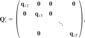
and ΔWi and ΔWi,−1 are (T − 1) × m-dimensional matrices,

and

The standard GMM estimator of φ = vec(Φ) is now given by17
An alternative estimator of

also used in the literature is given by

. See, for example, Arellano and Honoré (2001) and Baltagi (2001). However, our Monte Carlo experiments suggest

to be preferable in the settings we consider, particularly for purposes of hypothesis testing. Arellano and Honoré (2001) also discuss how auxiliary assumptions can be used to impose further restrictions on

.

where

and

, where

is an initial consistent estimate of Φ such as the generalized instrumental variables estimator obtained using the formula (6.4) but with

replaced by ΛQ [otimes ] Im, where

and

is the (T − 1) × (T − 1) matrix,
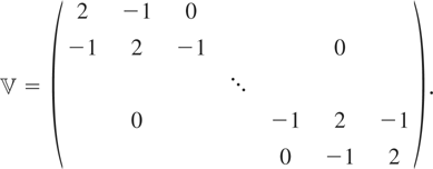
Because the resultant instrumental variables estimator is invariant to the choice of Ωε, without loss of generality the estimator may be computed replacing

by ΛQ [otimes ] Im. Using the standard formula, a consistent estimate of the variance matrix of

can be obtained as

The standard GMM estimator is consistent if all eigenvalues of Φ fall inside the unit circle but breaks down if some eigenvalues of Φ are equal to unity. Note that a necessary condition for the GMM estimator (6.4) to exist is that rank(Qi′ΔWi,−1) = m as N → ∞. In the case where Φ = Im, rank(Qi′ΔWi,−1) as N → ∞ is less than m, however. This is because when Φ = Im, for t = 2,3,…,T we have Δwit = εit, and wit = wi0 + sit, with

, and thus it follows that for t = 2,3,…,T, l = 0,1,…,t − 2, as N → ∞

where

denotes convergence in probability. In other words, when Φ = Im, the elements of qit, although still uncorrelated with the equation errors, are also uncorrelated with the regressors.
18The same conclusion holds for PVAR(p) models, with more complicated derivation. A note containing a detailed argument is available from the authors upon request.
Nevertheless, a consistent GMM-type estimator may be obtained by making use of additional moment conditions. One possibility is the estimator proposed by Ahn and Schmidt (1995, 1997), which augments the standard moment conditions with those implied by homoskedasticity assumptions as in Assumption (G2). These are legitimate instruments regardless of the unit root and cointegrating properties of wit − μi. In the context of (2.1) and under homoskedasticity (over time) of the εit's we have the following additional sets of moment conditions:

and

where

Arellano and Bover (1995) and Blundell and Bond (1998) proposed an additional set of moment conditions that in the case of model (2.1) can be written as

It is readily seen that these conditions require that

Thus, unless Φ = Im, the moment conditions (6.10) involve restrictions on the distribution of the initial observations, wi0, and assume that the individual effects and the disturbances are uncorrelated. The Ahn and Schmidt (1995, 1997) homoskedasticity implied moment restrictions (equations (6.7) and (6.8)), and the Arellano and Bover (1995) and Blundell and Bond (1998) initialization restrictions implied moment conditions (equation (6.10)), can now be combined, after eliminating redundant conditions, to yield the following moment conditions that are linear in Φ:

together with the conditions set out in (6.10).
The extended GMM estimator of Φ can now be based on the moment conditions (6.1), (6.10), and (6.11), which we write in stacked form as

where Pi′ is a matrix of dimension [mT(T − 1)/2 + 2m(T − 1)] × T,

with P1i a matrix of dimension mT(T − 1)/2 × T given by

P2i a matrix of dimension m(T − 1) × T given by

P3i a matrix of dimension m(T − 1) × T given by

and Wi and Wi,−1 are T × m-dimensional matrices,
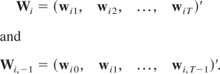
The extended GMM estimator of φ = vec(Φ) is now given by

where

and

, where

is an initial consistent estimator of Φ, for example, the generalized instrumental variables estimator based on (6.12), but with

replaced by ΛP [otimes ] Im, where

Using the standard formula, a consistent estimate of the variance-covariance matrix of the extended GMM estimator (6.12) can be obtained as

Remark 6.1. The GMM estimators (6.4) and (6.12) require that the second moments of μi exist. For asymptotic normality of these estimators it will also be required that the fourth moments of μi exist. The existence of these moments is not implied by any of the assumptions we had invoked for QML estimation under the fixed effects specification. Moreover, the number of moment conditions for GMM increases at the order of T2, whereas the orthogonality conditions for QML estimation remain the same as T increases, which can have implications for the finite-sample performance of the two types of estimators.
Remark 6.2. The efficiency of the GMM estimators depends on the correlations between the instruments, wi0,wi1,…,wi,t−2, and the regressors, Δwi,t−1. We show in the Appendix that in the stationary case the asymptotic variance of the standard GMM estimator is an increasing function of Ωμ, the variance matrix of the individual effects, relative to the variance matrix of

, Ωξ, in the sense that for any two variance matrices, Ωμ(1) and Ωμ(2), conditional on a given choice of Ωξ,

if Ωμ(1) − Ωμ(2) ≥ 0, and vice versa, where ≥ stands for a positive semidefinite matrix.19
In Binder et al. (2004, Appendix B), we show that in the pure unit root case the asymptotic variance of the extended GMM estimator similarly is an increasing function of Ωμ relative to Ωε.
Remark 6.3. To ensure that the efficiency of GMM does not depend on the nuisance parameters, Ωμ, one may reformulate standard GMM using Δwi,t−2, Δwi,t−3,…,Δwi1 as instruments (an estimator that might be referred to as FE-GMM). However, such a FE-GMM estimator still cannot be as efficient as QMLE as the former uses linear combinations of Δwi,t−2,Δwi,t−3,…,Δwi1 as instruments whereas the latter uses linear combinations of Δwi,t−1, Δwi,t−2,…, Δwi1 as instruments for Δwi,t−1. Moreover, if one or more characteristic roots of the underlying PVAR are close to unity, the correlations between Δwi,t−1 and Δwi,t−2,Δwi,t−3,… would be small; hence GMM using lagged first-differenced variables may be highly inefficient. On the other hand the efficiency of FE-QMLE is not affected by the value of the characteristic roots because Δwi,t−1 is one of the instruments for Δwi,t−1.
Remark 6.4. As is well known from the instrumental variables literature, asymptotic efficiency results in any case need not carry over to small or even moderate sized samples, particularly when the number of moment conditions is large relative to the number of observations. The extended GMM estimators seem to be subject to such a shortcoming. This is because in the absence of prior information on the unit root properties of wit all moment conditions could be informative,20
In the single equation context, Wansbeek and Bekker (1996) argue the importance of using all applicable moment conditions; Hahn (1999) argues that the information content of the homoskedasticity implied moment conditions is significantly augmented if initialization restrictions are imposed.
The use of more moment conditions can lead to an increase in the bias of the GMM estimators in finite sample; for example, see Ziliak (1997).
We thus turn next to an examination of the finite-sample properties of the QML estimators and also standard and extended GMM estimators by means of Monte Carlo experiments.22
Although we consider a fairly broad range of model specifications,23
A number of model specifications not considered in this section, together with the case of nonnormal errors, are available in Binder et al. (2004).
We consider three types of designs for the matrix of slope coefficients, Φ. These designs distinguish between stationary, pure unit root, and cointegrated PVAR models. In the case of stationary designs we consider three subcases with Φ having maximum eigenvalues equal to 0.6, 0.8, and 0.95. For all designs we set m = 2, and to make the Monte Carlo results from the various designs comparable, we specify (where appropriate) different error variance matrices for different designs so as to obtain similar population R2 values for both equations of the PVAR model and across all designs.
Design 1a: Stationary PVAR with maximum eigenvalue of Φ equal to 0.6

The other eigenvalue of Φ is 0.2, and the population R2 values are given by R[utri ]wlit2 = 0.2364, l = 1,2, i = 1,2,…,N, and t = 2,3,…,T, where

with

denoting the element in the lth row and lth column of the matrix

.
24See Pesaran, Shin, and Smith (2000) for a discussion of the computation of R2 values for (possibly cointegrated) VARs.
Design 1b: Stationary PVAR with maximum eigenvalue of Φ equal to 0.8

The other eigenvalue of Φ is 0.4, and the population R2 values are given by R[utri ]wlit2 = 0.2396, l = 1,2, t = 2,3,…,T, where R[utri ]wlit2 are computed as in (7.1).
Design 1c: Stationary PVAR with maximum eigenvalue of Φ equal to 0.95

The other eigenvalue of Φ is 0.45, and the population R2 values are given by R[utri ]wlit2 = 0.2383, l = 1,2, t = 2,3,…,T, where R[utri ]wlit2 are computed as in (7.1).
Design 2: PVAR with unit roots (but noncointegrated)

Design 3: Cointegrated PVAR

The eigenvalues of Φ in this case are given by 1 and 0.6, and the implied vectors/matrices α, β, and Π are given by

The population R2 values are given by R[utri ]wlit2 = 0.2381, l = 1,2, t = 2,3,…,T, where R[utri ]wlit2 are computed as in (7.1).
The baseline settings across all five designs for the remaining model parameters are as follows. We take the εit's to be normally distributed, and we generate the individual-specific effects as

with

being distributed independently of εit for all i and t. In this way the individual effects will not be normally distributed. Clearly, the particular way that the individual effects are generated has no consequence for the FE-QMLE but could be important for the GMM-type estimators. For τ we consider two values, τ = 1 and 5. It should be recalled that τ measures the degree of cross-section to time-series variations, which can be large in economic applications (for some evidence, see, e.g., the estimates provided in Tables I–IV of Lee, Pesaran, and Smith, 1997, and the figures in Hsiao, Shen, and Fujiki, forthcoming). The Monte Carlo studies of GMM estimators in the univariate context typically set τ = 1. The properties of the FE-QMLE do not depend on τ.
The wit's were generated using (2.1) and the initialization

with C = β⊥(α⊥′ β⊥)−1α⊥′ and where α⊥ and β⊥ are m × (m − r) matrices of full column rank such that α′α⊥ = 0 and β′β⊥ = 0; also

. Under this initialization we have that R[utri ]wli12 = R[utri ]wlit2, for t = 2,3,…,T, and l = 1,2.
25See Binder et al. (2004) for further discussion of this initialization scheme, which ensures that the same processes generating the stationary components of {ξit}t=1T also generate those of ξi0, and the same processes generating the common stochastic trend components of {ξit}t=1T also generate those of ξi0.
In further experiments we consider a couple of deviations from the baseline scenario. As a partial analysis of the performance of the QML estimator under nonnormal disturbances we consider the cases of t- and chi square distributed disturbances (see Binder, Hsiao, and Pesaran, 2004). Also, as a partial analysis of the information content of the moment conditions available under the random but not the fixed effects specification, we compare the FE-QMLE and RE-QMLE under cross-sectionally homoskedastic individual-specific effects, generating the latter as

, with

again being distributed independently of εit for all i and t, and τ = (1, 5).
In what follows we compare the various estimators in terms of their biases and root mean square errors (RMSEs). We also investigate the finite-sample performance of a number of tests based on these estimators. For Designs 1 and 2 we compute the various estimators with Π unrestricted, and for Design 3 we compute the QML estimator both with and without imposing rank restrictions on Π. In what follows we refer to the GMM estimator that uses only the orthogonality and initialization restrictions implied moment conditions as the extended GMM estimator I and to the GMM estimator that uses only the orthogonality and homoskedasticity implied moment conditions as the extended GMM estimator II. Finally, the GMM estimator that uses the orthogonality, initialization restrictions, and homoskedasticity implied moment conditions will be referred to as the extended GMM estimator III. A summary of the computational details is provided in Binder et al. (2004).
The evidence on the finite-sample properties of the various estimators in the case of normally distributed disturbances and when no rank restrictions are imposed on the matrix Π are summarized in Tables 1 and 2. Performance of each estimator is evaluated according to the familiar four criteria, namely, bias, RMSE, size, and power. Table 1 reports the bias and RMSEs of the various estimators. To economize on space we focus on the results for the elements in the first column of Φ, namely, φ11 and φ21. The results for φ12 and φ22 are qualitatively similar and are available upon request. Size and power of the tests are reported in Tables 2a, 2b, 2c, and 2d. The nominal size is set to 5%. Once again to save space Tables 2a, 2b, 2c, and 2d only report the results for Designs 1a and 3. For the GMM-type estimators we report the results for τ = 1 and 5.
Bias and RMSE of alternative estimators of panel VAR

Size and power properties of tests for φ11 under alternative estimators of panel VAR, λmax = 0.6

Size and power properties of tests for φ21 under alternative estimators of panel VAR, λmax = 0.6

Size and power properties of tests for φ11 under alternative estimators of panel VAR, λmax = 1

Size and power properties of tests for φ21 under alternative estimators of panel VAR, λmax = 1

The results in Tables 1 and 2 clearly show that the performance of the GMM-type estimators tends to deteriorate with increases in τ, except in the pure unit root case. These simulation results are in line with our theoretical derivations discussed in Remark 6.2 and will not disappear if larger sample sizes are considered. The FE-QMLE is invariant to changes in τ, and its finite-sample performance is therefore unaffected by the choice of τ. The dependence of the GMM-type estimators on τ and/or on whether Φ = I2 complicates the comparison of the various estimators. However, our Monte Carlo results suggest that even when τ is relatively small, τ = 1, the FE-QMLE tends to perform significantly better than the GMM-type estimators, possibly with the exception of the extended GMM estimators in the pure unit root case. Although for a small number of scenarios with τ = 1 one or more of the extended GMM estimators on a subset of our four evaluation criteria perform slightly better than the FE-QMLE, the differences in performance in those cases tend to be small and are outweighed or at least offset by reverse ranking on one or more of the other evaluation criteria.26
At the suggestion of a referee, we also carried out a Monte Carlo study of the FE-GMM estimator discussed in Remark 6.3. This estimator performed considerably worse than the standard GMM estimator, and to save space we are not including it in the result tables.
The results in Tables 1 and 2 also confirm the breakdown of the standard GMM estimator in the presence of unit roots and document its deterioration as the eigenvalues of Φ approach unity, even for the relatively large sample size of N = 250, T = 10. None of the extended GMM estimators suffers from this problem. In fact, ceteris paribus the extended GMM estimators perform best in the pure unit root case. Of the various extended GMM estimators, the one using the homoskedasticity but not the initialization restrictions (extended GMM estimator II) is least sensitive to changes in τ. The tests based on extended GMM estimators I and III suffer from a considerable degree of overrejection when T = 10, particularly as τ is increased. This finding should not be too surprising given that the standard orthogonality conditions and also the initialization restrictions implied moment conditions involve interaction terms involving both levels and first differences, whereas the homoskedasticity implied moment conditions only involve levels terms. The finding that the extended GMM estimator II is relatively robust to changes in τ is unfortunately of limited use for empirical analysis, however, as the extended GMM estimator II performs worse than the other two extended GMM estimators when smaller values of τ are considered. Also, it is worth noting that although for τ = 1 the extended GMM estimators outperform the standard GMM estimator, as τ increases this ranking is reversed in some instances. Finally, the results show that the performance of the GMM-type estimators need not improve as T is increased. This is due to the rapid increase in the number of legitimate instruments with T, and it stands in contrast to the FE-QMLE, whose performance invariably improves with T. In summary, the Monte Carlo results suggest that the GMM estimators are likely to perform well if prior knowledge is available regarding the location of the eigenvalues of Φ and/or if it is known that τ is small (so that the most suitable moment conditions could be picked). However, even in cases where the GMM estimators perform reasonably well in terms of bias and RMSE, they tend to be outperformed by the FE-QMLE in terms of size and power of the tests, except in the pure unit root case. The extended GMM estimators, however, provide useful consistent initial estimates for the QML estimation iterations.27
We also followed up on a further suggestion of a referee and considered GMM estimators with randomly selected moment conditions. We examined a number of alternative moment selection procedures. But none of these GMM estimators outperformed the corresponding GMM estimators based on all the valid moment conditions. However, a comprehensive examination of the subset moment selection procedure as a possible means of improving the finite-sample performance of the various GMM estimators is beyond the scope of this paper.
Overall, the results show that the FE-QMLE performs well and is remarkably robust to the time-series properties of the underlying variables. In particular, the performance of the FE-QMLE is generally unaffected by whether the maximal eigenvalue of Φ is moderately sized, close to, or equal to unity.
Table 3 presents evidence on the finite-sample properties of the FE-QMLE in the case of a cointegrated PVAR model (Design 3). We did not compute any of the GMM estimators for this design: the main virtue of the GMM estimators, their computational simplicity, is lost in the presence of rank restrictions on Π, as in such cases the GMM estimators would have to be computed using iterative optimization techniques. The results in Table 3 show that the FE-QMLE continues to perform reasonably well under rank restrictions on Π. Nevertheless, it should be noted that in the smallest sample (N = 50, T = 3) the RMSEs for the FE-QMLE tend to be larger than for the other designs and the test of cointegration rank is undersized. For larger sample sizes featuring a larger N and/or T, bias and RMSE diminish rather rapidly, however, and size and power properties of the tests improve considerably.
Table 3a. Bias and RMSE of fixed effects QML estimator of cointegrated panel VAR
Table 3b. Size and power properties of cointegration rank tests based on fixed effects QML estimator

Table 3c. Size and power properties of tests for α1 under fixed effects QML estimator of cointegrated panel VAR
Table 3d. Size and power properties of tests for α2 under fixed effects QML estimator of cointegrated panel VAR
Table 3e. Size and power properties of tests for β2 under fixed effects QML estimator of cointegrated panel VAR

We have also carried out Monte Carlo studies on the performance of the FE-QMLE under two types of departures from normally distributed disturbances, namely, when the disturbances are t(5) or χ2(1) distributed.28
Because these two types of departure from normality cover both the possibility of fat tails and the possibility of an asymmetric/skewed shock distribution, it is very likely that the results could be of greater generality.
We also obtained broadly similar results for the various GMM estimators.
All of the preceding arguments carry over to the random effects setting. Our Monte Carlo studies revealed that under the random effects model the FE-QMLE performs on a par with the RE-QMLE even for the smallest sample size (N = 50, T = 3). The differences between the two estimators are very small across all the four evaluation criteria, often even favoring the FE-QMLE. Thus, the argument often advanced concerning the efficiency loss involved in the first-differencing operation that underlies the FE-QMLE as compared to the RE-QMLE does not appear to be important for the estimation of PVARs using finite samples. The RE-QMLE, however, remains the estimator of choice if the primary purpose of the analysis is the identification and estimation of the effects of time-invariant variables in short panels. In that case great caution must be exercised because the random effects model imposes strong assumptions on the distribution of the individual-specific effects. For the identification and estimation of the effects of time-varying variables our findings favor the use of FE-QMLE on grounds of its robustness to any form of specification of the distribution generating the individual-specific effects.
In this paper, we have extended the analysis of linear dynamic panel data models with short time dimension in a number of respects. We have generalized the extended GMM estimators, hitherto studied in the literature in a single equation context, to a multivariate PVAR setting. We have derived random and fixed effects QML estimators and have shown that the QML estimators are consistent and asymptotically normally distributed when the cross-sectional dimension of the panel approaches infinity, irrespective of whether the underlying time series are (trend) stationary, pure I(1), or I(1) and cointegrated. Furthermore, we have proposed new QML-based procedures for conducting tests for unit roots and cointegration rank in panels with short time dimension and have shown that the limiting distributions of the relevant test statistics follow standard chi square and normal distributions.
The applicability of the various GMM estimators requires that certain assumptions on the unobserved individual effects are satisfied. From the perspective of empirical analysis, these assumptions could be restrictive. In addition, the Monte Carlo evidence presented in Section 7 favors the FE-QMLE over the various GMM estimators, even under important departures from normally distributed disturbances. The finite-sample performance of the various GMM estimators depends critically on a ratio reflecting unobserved cross-section variation in the data relative to unobserved time-series variation, but even if this ratio is relatively small the GMM estimators are outperformed in finite sample by the QML estimators. A theoretical rationale is also provided for this result whereby it is shown that the asymptotic variance of the GMM estimators is an increasing function of the variance of the individual effects, whereas the distribution of the FE-QMLE is invariant to the size of this variance.
The use of likelihood-based procedures for estimation and inference in VAR models is standard in the time-series literature. This paper has provided both theoretical and operational arguments for the application of likelihood-based methods to PVAR models, whether the underlying time series are stationary, integrated, or cointegrated. The ultimate test of our approach lies in the application of the proposed techniques to substantive economic problems. This is the next stage of our research and hopefully that of others. The likelihood approach can also be used to address other theoretical issues of interest, such as model selection and conditional estimation and inference in PVARs.
In this Appendix we derive the asymptotic variance of

, the standard GMM estimator defined by (6.4), as N → ∞, and show that it is an increasing function of Ωμ, the variance matrix of the individual effects, μi, in the sense that if Ωμ(1) − Ωμ(2) is a positive semidefinite matrix, so will be

where Ωμ(j), j = 1,2, are two different variance matrices for the individual effects. (The more complicated case of the dependence of extended GMM on Ωμ can be derived similarly noting that wit − Φwi,t−1 = (I − Φ)μi + εit and making use of the relations (6.10) and (6.11).)
The asymptotic variance of

is given by (also see (6.6))

where Ωε = E(εitεit′),
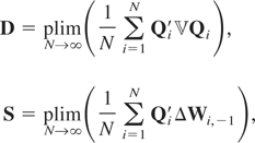
and

are defined by (6.2), (6.3), and (6.5), respectively.
To simplify the derivations we suppose that Assumptions (G1), (G2), and (R1) hold, that all eigenvalues of Φ fall inside the unit circle, and that the wit process has started in the infinite past. Under these assumptions (the results will be qualitatively unaffected if one considers other initializations of the wit process discussed in Binder et al., 2004)

and it is easily seen that


where

. Also under Assumption (G2)

Using (A.1) and (A.2) we have

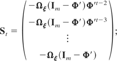
with St, for t = 2,3,…,T, a matrix of dimension m(t − 1) × m given by
furthermore we have

where

is a matrix of dimension T(T − 1)/2 × T(T − 1)/2 given by

ιt being a vector of ones of dimension t × 1, for t = 1,2,…,T − 1, and where H is a matrix of dimension mT(T − 1)/2 × mT(T − 1)/2 given by

with Htt, for t = 2,3,…,T, a matrix of dimension m(t − 1) × m(t − 1) given by

Ht,t+1, for s = 2,3,…,T, a matrix of dimension m(t − 1) × m(t − 1) given by

and Ht+1,t, for s = 2,3,…,T, a matrix of dimension m(t − 1) × m(t − 1) given by

It is clear that

will depend on Ωμ only through the matrix D, and for any two variance matrices, Ωμ(j), j = 1,2,

if

where

denotes that A − B is a positive semidefinite matrix. This condition implies

and because S does not depend on Ωμ(j), using (A.3) the condition (A.4) will be satisfied if

or if Ωμ(1) ≥ Ωμ(2). The preceding sequence can be reversed to show that if Ωμ(1) ≥ Ωμ(2) then (A.4) will follow.
In the simple case where m = 1 and T = 3, we have

and after some algebra it follows that

where τ = σμ2/σε2. It is interesting to note that

depends on the ratio τ and not the error variances σμ2 and σε2 separately. It is also easily established that

is an increasing function of τ, for all values of |φ| < 1 and τ > 0.

Bias and RMSE of alternative estimators of panel VAR

Size and power properties of tests for φ11 under alternative estimators of panel VAR, λmax = 0.6

Size and power properties of tests for φ21 under alternative estimators of panel VAR, λmax = 0.6

Size and power properties of tests for φ11 under alternative estimators of panel VAR, λmax = 1

Size and power properties of tests for φ21 under alternative estimators of panel VAR, λmax = 1

Table 3a. Bias and RMSE of fixed effects QML estimator of cointegrated panel VARTable 3b. Size and power properties of cointegration rank tests based on fixed effects QML estimator

Table 3c. Size and power properties of tests for α1 under fixed effects QML estimator of cointegrated panel VARTable 3d. Size and power properties of tests for α2 under fixed effects QML estimator of cointegrated panel VARTable 3e. Size and power properties of tests for β2 under fixed effects QML estimator of cointegrated panel VAR