

Dinosaurs are one of the most charismatic and heavily studied groups of vertebrates (e.g., Sereno Reference Sereno1999), but despite ongoing work and many recent discoveries, certain aspects of early dinosaurian evolution remain unclear. A recent study of early dinosaur relationships presented a new phylogeny that departs radically from existing models, but forms a broader framework for inferring dinosaur evolutionary history than those that were previously available (Baron et al. Reference Baron, Norman and Barrett2017a). While that study was focused primarily on early dinosaurian anatomy and relationships, a general observation was made: based upon the geographic locations of key taxa in their phylogeny, a Laurasian setting for dinosaur origin may have been plausible. This proposal ran contrary to an established consensus based on earlier phylogenies that favoured a Gondwanan and, more specifically, South American setting for this event (Nesbitt et al. Reference Nesbitt, Smith, Irmis, Turner, Downs and Norell2009; Brusatte et al. Reference Brusatte, Nesbitt, Irmis, Butler, Benton and Norell2010; Langer et al. Reference Langer, Ezcurra, Bittencourt and Novas2010; Sues et al. Reference Sues, Nesbitt, Berman and Henrici2011; Boyd Reference Boyd2015). In particular, the European presence of silesaurids, a close outgroup to dinosaurs, and some early dinosaur taxa (e.g., Saltopus) hinted that northern Pangaea may have played an important role in the earliest stages of dinosaur diversification. However, given the space limitations associated with the original article, no quantitative analyses were carried out to evaluate this alternative hypothesis rigorously.
Here, we test the alternative hypothesis implicit in Baron et al. (Reference Baron, Norman and Barrett2017a) by analysing their early dinosaur dataset using a novel integration of time-sliced Bayesian biogeographic models (Landis Reference Landis2016) and tip-dated Bayesian phylogenetics (Drummond et al. Reference Drummond, Suchard, Xie and Rambaut2012; Bielejec et al. Reference Bielejec, Baele, Rambaut and Suchard2014; Gavryushkina et al. Reference Gavryushkina, Heath, Ksepka, Stadler, Welch and Drummond2017). The current method simultaneously estimates phylogenetic relationships, divergence dates, evolutionary rates and biogeographic patterns. Biogeographical changes are inferred using models that account for the changing relationships of continents (and thus dispersal abilities) over time – a ‘chronobiogeographical' paradigm (Hunn & Upchurch Reference Hunn and Upchurch2001) – and this information provides potentially critical information for improving estimates of tree topology and divergence dates. For comparison, we also perform analogous analyses using traditional biogeographic parsimony-based methods.
Previous studies have advocated a similar approach to integrating phylogeny, stratigraphy, morphology and biogeography in a parsimony framework (reviewed in Rossie & Seiffert Reference Rossie, Seiffert, Lehman and Fleagle2006). However, that implementation was problematic: as parsimony trees lack an explicit time element, only very simple time-sliced biogeographic models were possible (e.g., three areas and three time slices) and tree topology and divergence dates had to be assessed manually. The analyses attempted here tackle this complex multidimensional problem more efficiently, using explicit Bayesian computational approaches.
1. Material and methods
1.1. Morphological, stratigraphic and biogeographic data
Morphological data were derived from the matrix of Baron et al. (Reference Baron, Norman and Barrett2017a), with 457 characters coded for 73 taxa (supplementary File 1 available at https://doi.org/10.1017/S1755691018000920). Euparkeria was designated as the outgroup to all other taxa in all Bayesian and parsimony analyses, as previously. The fragmentary early dinosauriform Nyasasaurus (Nesbit et al. Reference Nesbitt, Barrett, Werning, Sidor and Charig2013) was not included as it is being re-studied and may be a chimera (M.G.B., P.M.B. and S. Nesbitt, unpub. data). Changes unique to terminal branches (autapomorphies) were explicitly sampled in this dataset, comprising >10 % of the characters, making this matrix especially appropriate for tip-dated Bayesian approaches (Lee & Palci Reference Lee and Palci2015).
Stratigraphic and biogeographic data were obtained for each terminal taxon (supplementary File 2). These data are compiled and presented in full in Baron (Reference Baron2018, Appendix 1). The stratigraphic data consisted of ranges (minimum and maximum ages) rather than point ages, thus allowing the dated analyses to account for stratigraphic uncertainty. Biogeographic data consisted of locality information categorised into the 25 broad tectonic regions employed in Landis (Reference Landis2016), which explicitly models the changing connectivities of these regions through 26 epochs of geological time spanning the entire Phanerozoic.
1.2. Bayesian tip-dated analyses using time-sliced biogeographic models
A novel recent study (Landis Reference Landis2016) united statistical biogeography with divergence dating: inferred dispersal events on a phylogeny would be expected to exhibit maximum concordance with palaeobiogeography when that phylogeny is correctly time scaled. That study used biogeographic data and time-sliced mode-weighted dispersal matrices (see below) to estimate absolute divergence dates, in the relatively simple situation involving an undated ultrametric tree of fixed topology and fixed relative branch lengths (based on published molecular analyses). In this article we demonstrate that this approach can be integrated into a more complex situation that involves a non-ultrametric, tip-dated phylogeny in which both topology and relative branch lengths are being co-estimated using additional data. In this more complex situation, the biogeographic information does not solely dictate absolute dates; rather, this has to be co-estimated in combination with other information on tip dates, morphological data and clock model, tree and fossil sampling, priors, etc. Since tree topology and relative branch lengths are not fixed, the biogeographic information can, and will, influence both aspects, especially for parts of the tree where the signal from other data is weak.
The morphological, stratigraphic and biogeographic data were simultaneously analysed using tip-dated Bayesian analyses (Drummond & Suchard Reference Drummond and Suchard2010; Ronquist et al. Reference Ronquist, Klopfstein, Vilhelmsen, Schulmeister, Murray and Rasnitsyn2012; Gavryushkina et al. Reference Gavryushkina, Heath, Ksepka, Stadler, Welch and Drummond2017). The optimal evolutionary histories that explain all three data sources were inferred using Markov chain Monte Carlo (MCMC) approaches as implemented in BEAST 1.8.4. BEAST (Suchard et al. Reference Suchard, Lemey, Baele, Ayres, Drummond and Rambaut2018) was used because it is increasingly widely employed for tip-dated phylogenetic analysis of time-sampled data including fossils (e.g., Drummond & Suchard Reference Drummond and Suchard2010; Gavryushkina et al. Reference Gavryushkina, Heath, Ksepka, Stadler, Welch and Drummond2017), can implement time-sliced biogeographic models (currently BEAST 1 only: Bielejec et al. Reference Bielejec, Baele, Rambaut and Suchard2014) and can also implement random local clocks (Drummond & Suchard Reference Drummond and Suchard2010), which are suitable for assessing clade-specific rates of change in single traits such as biogeography (Sanders et al. Reference Sanders, Rasmussen, Mumpuni Elmberg, de Silva, Guinea and Lee2013; King & Lee Reference King and Lee2015). The executable BEAST XML files, with annotations describing model, prior, MCMC and logging settings, are in supplementary Files 3–5. The description below summarises the major points, focusing on the biogeographic data and models.
In all Bayesian analyses, the morphological characters were analysed using the Mk model with correction for non-sampling of constant characters (Lewis Reference Lewis2001; Alekseyenko et al. Reference Alekseyenko, Lee and Suchard2008), which has been well tested (Wright & Hillis Reference Wright and Hillis2014; O'Reilly et al. Reference O'Reilly, Puttick, Parry, Tanner, Tarver, Fleming, Pisani and Donoghue2016). 47 characters were autapomorphies (variable but parsimony uninformative), and only six were invariant (thus, invariant characters were essentially unsampled). Polymorphic morphological data (0 and 1) could be treated exactly as scored (e.g., 0 or 1 but not 2) not as total uncertainty (0 or 1 or 2): an improvement over earlier versions of BEAST. 418 morphological characters were treated as unordered and 39 characters forming morphoclines were treated as ordered (see list in Baron et al. Reference Baron, Norman and Barrett2017a).
We tested both an unpartitioned model and a state-partitioned model for the morphological data (Gavryushkina et al. Reference Gavryushkina, Heath, Ksepka, Stadler, Welch and Drummond2017): both yielded similar results. We present both results but focus on the unpartitioned model, as employing a single five-state substitution Lewis model for all traits ensures all state transitions were weighted identically, even for characters with different numbers of observed states. Partitioning characters according to the number of observed states can result in better model fit, but has minimal effect on phylogeny, dates or ancestral state reconstruction on datasets tested thus far (e.g., Gavryushkina et al. Reference Gavryushkina, Heath, Ksepka, Stadler, Welch and Drummond2017; King et al. Reference King, Qiao, Lee, Min and Long2017). Furthermore, such state-partitioned models have potential drawbacks: (1) they increase the influence of characters with more states (e.g., King et al. Reference King, Qiao, Lee, Min and Long2017); and (2) unless homoplasy is exceptionally rampant, the observed states of a character might not represent all possible states (Hoyall Cuthill Reference Hoyal Cuthill2015). Indeed, in related outgroups (Ksepka et al. Reference Ksepka, Fordyce, Ando and Jones2012), increased state space can be observed for many of the characters modelled in Gavryushkina et al. (Reference Gavryushkina, Heath, Ksepka, Stadler, Welch and Drummond2017). As a further example, most sites in amino acid alignments will not exhibit all 20 possible states, and many DNA alignments will have sites with fewer than four states (amino acid or DNA alignments are not typically analysed by assuming that the observed states at each variable position are the only possible states).
Bayes factors (BF) (sensu Kass & Raftery Reference Kass and Raftery1995), calculated using stepping-stone sampling (Xie et al. Reference Xie, Lewis, Fan, Kuo and Chen2011), found significant variation in rates of morphological evolution across different characters, favouring the inclusion of the gamma parameter (Yang Reference Yang1994) for among-character rate variation (BF ∼130). We used a gamma rather than log-normal distribution (Harrison & Larsson Reference Harrison and Larsson2015) because the gamma distribution can be parameterised to resemble any log-normal distribution (but not the reverse). There was also significant variation in rates of morphological evolution across different lineages, with a relaxed (uncorrelated log-normal; Drummond et al. Reference Drummond, Ho, Phillips and Rambaut2006) clock preferred over a strict clock (BF ∼220). However, there was no evidence that different dinosauromorph lineages had different rates of dispersal: for the biogeographic data, a relaxed (random local; Drummond & Suchard Reference Drummond and Suchard2010) clock did not fit better than a strict clock (strict clock slightly favoured, BF <5). Thus, all Bayesian analyses employed the gamma parameter and relaxed clock for the morphological data, but a strict clock for the biogeographic character.
The most appropriate available tree prior in BEAST 1.8 was used (birth–death serial sampling of Stadler Reference Stadler2010; sampled ancestor tree priors only available in BEAST2). Tip calibrations were employed using the full stratigraphic range for each taxon, with each taxon's age being represented by a uniform prior spanning minimum–maximum ages. In the focal analysis, a hard constraint on maximum root age was employed for the main analyses described: 259.9Ma. This represents the oldest potential fossil for the much larger clade Archosauriformes (Bernardi et al. Reference Bernardi, Klein, Petti and Ezcurra2015), and substantially exceeds the age of the oldest fossils analysed here. However, additional analyses, where the root age constraint was changed to a looser (soft exponential) constraint, did not change the phylogenetic and biogeographic conclusions. There was no explicit minimum root age constraint; this was dictated by the oldest included fossil (∼124Ma).
The biogeographic data were treated as a discrete character in a separate partition, with 25 states corresponding to the tectonic provinces listed in Landis (Reference Landis2016), a necessary simplification due to the available functionality in BEAST (see Discussion). Two main Bayesian analyses were performed, in which the biogeographic data scored for the terminal taxa was treated in very different ways, to test the robustness of the results generated by different models.
1.2.1. Dynamic, time-sliced biogeographic model (Landis Reference Landis2016)
This model recognises that the rate of dispersal between the 25 areas increases with greater connectivity, i.e., decreasing distance and absence of water barriers (as dinosaurs are essentially terrestrial, e.g., Poropat et al. Reference Poropat, Mannion, Upchurch, Hocknull, Kear, Kundrat, Tischler, Sloan, Sinapius, Elliott and Elliott2016). Twenty-five (25) areas have 300 possible connections between area pairs, assuming reversibility (above-diagonal elements of a 25×25 matrix). These 300 connections were classified as consistent with short-range, medium-range or long-range dispersal. Distances between area pairs, however, vary through time due to tectonic motion, eustatic fluctuations and changes to the areal extent of shelf seas, resulting in a dynamic or time-heterogeneous dispersal model. Landis (Reference Landis2016) defined connectivities for 26 time slices or ‘epochs': epochs 7–12 span the time interval relevant to this study (280–120Ma) and are used here. They are here renumbered as epochs 1–6 respectively; the age boundaries of all epochs are shown in Figure 1 and their connectivities in supplementary Figure 1.
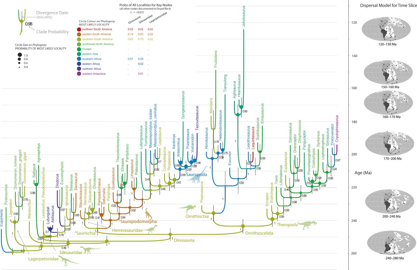
Fig. 1 ‘Dynamic' time-sliced biogeographic model of early dinosaur evolution based on Bayesian tip-dated analysis of the data matrix in Baron et al. (Reference Baron, Norman and Barrett2017a). Ancestral areas were inferred accounting for changing continental connections; dispersals between adjacent areas are favoured, but connectivities of areas change as per plate tectonics. The model recovers a South American origin of Dinosauria but with non-trivial probability for closely adjacent areas. (Lagerpetid silhouette by Nobu Tamara from phylopic.org; maps after Landis Reference Landis2016; all other images the authors.)
Short-, medium- or long-range dispersals are assigned separate relative rates; areas linked by short-range dispersal are also linked by medium- and long-range dispersal, areas linked by medium-range dispersal are also linked by long-range dispersal (Landis Reference Landis2016, Fig. 4). Thus, under all possible parameterisations, this yields the intuitive pattern that dispersal rates between areas separated by short distances exceed the dispersal rates of those areas separated by medium distances, which in turn exceed the dispersal rates between areas separated by long distances. The summed (but still relative) dispersal rates between all 600 area pairs are thus encoded into a mode-weighted dispersal matrix for each of the 26 time slices (resulting in 26 dispersal matrices, of which matrices 7–12 are relevant here). In Landis (Reference Landis2016), the relative rates of short-, medium- or long-range dispersals were empirically estimated using RevBayes; when implemented in BEAST using the epoch substitution model (Bielejec et al. Reference Bielejec, Baele, Rambaut and Suchard2014) on a 25×25 reversible general substitution matrix (Lemey et al. Reference Lemey, Rambaut and Drummond2009), these have to be fixed. We thus employ the empirical rates estimated in Landis (Reference Landis2016) that were for non-marine Testudines, a reptile group found in many of the same areas and time slices: short-range and medium-range dispersals have similar rates (average 0.49), and long-range dispersals have a much lower rate (0.02). This results in the following summed relative rates between pairs of areas in each time-sliced mode-weighted dispersal matrix:
• area pairs separated by short distances (short+med+long range dispersal)=1
• area pairs separated by medium distances (med+long range dispersal)=0.51
• area pairs separated by long distances (long range dispersal only)=0.02.
The mode-weighted dispersal matrices for the six epochs considered here (supplementary Fig. 1) are presented and annotated in the BEAST xml files.
As non-marine Testudines have traits that might be argued to make them more efficient overwater dispersers in comparison with non-avian dinosaurs (such as low metabolic rate, natural buoyancy), the analyses were repeated with lower values for medium and long range dispersal (0.1 and 0.01), with very similar results regarding topology, dates and ancestral areas.
1.2.2. Static, unordered model
This simple biogeographic model treats locality data in the same way as an unordered morphological character: every state (locality) can change to directly every other state (locality), and these changes happen at the same rate for all pairs of states. Thus, relative rates between all pairs of areas in the dispersal matrix are identical (arbitrarily set to unity), and this matrix also remains the same across all time slices. This is an extremely simple biogeographic model that has been argued to be far from realistic (e.g., Hunn & Upchurch Reference Hunn and Upchurch2001): for instance, dispersals between contiguous land areas are modelled to occur at the same rate as transoceanic dispersals. However, it continues to be regularly applied in biogeographic studies including those using Bayesian methods (e.g., Schaefer et al. Reference Schaefer, Hechenleitner, Santos-Guerra, de Sequeira, Pennington, Kenicer and Carine2012). Furthermore, as the most ‘distance-unweighted' and ‘time-homogeneous' possible dispersal model, it represents an extreme alternative to the distance-weighted, time-heterogeneous model implemented above.
In the two analyses described above (which considered biogeography under very different models), ancestral states were logged for all sampled trees; thus, in the consensus trees, the relative probabilities for each of the 25 areas was calculated for each ancestral node. These probabilities are shown for three key nodes (Dinosauria, Silesauridae, Lagerpetidae) in Figures 1 and 2; the values for all other nodes are in the consensus tree files (supplementary Files 7–10), which are best viewed using FigTree. Finally, to test the influence of incorporating biogeographic data at all (regardless of model), the Bayesian analysis was also repeated with the morphological and stratigraphic data only.
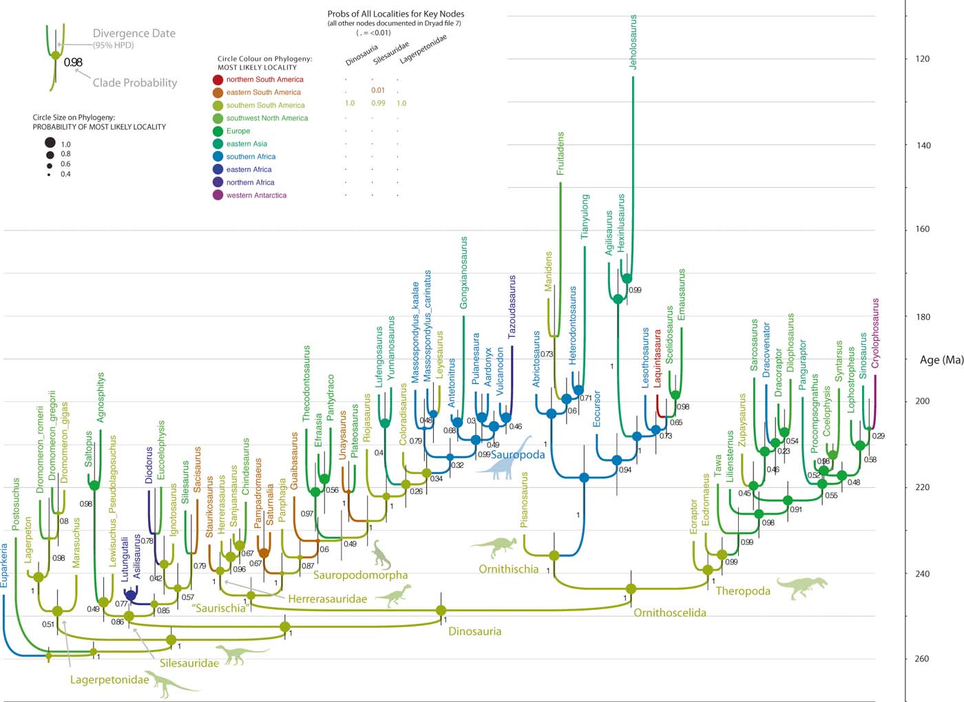
Fig. 2 ‘Static' biogeographic model of early dinosaur evolution based on Bayesian tip-dated analysis of the data matrix in (Baron et al. Reference Baron, Norman and Barrett2017a). Ancestral areas were inferred without accounting for changing biogeographic connections, so taxa move directly between all areas with equal probability in all time slices. Southern South America is recovered as the ancestral area for Dinosauria with unrealistically high certainty. (Lagerpertid silhouette by Nobu Tamara from phylopic.org; all other images the authors.)
All Bayesian analyses were run with a MCMC chain length of 50 million generations, with a burn-in of 20 % confirmed as adequate using Tracer (Rambaut et al. Reference Rambaut, Drummond, Xie, Baele and Suchard2018) and AWTY (Nylander et al. Reference Nylander, Wilgenbusch, Warren and Swofford2008). Analyses were replicated four times to confirm convergence, and the post-burn-in samples of all four runs concatenated for consensus trees and summary statistics with the aid of LogCombiner and TreeAnnotator (Drummond et al. Reference Drummond, Suchard, Xie and Rambaut2012) and FigTree (Rambaut Reference Rambaut2016). Executables to perform the above analyses are available as supplementary Files 3–6.
1.3. Parsimony analyses
Parsimony analysis and optimisation were also performed to compare the quantitative, probabilistic models with traditional cladistic approaches. We employed the standard sequential approach of parsimony analysis of phylogeny using morphological data alone, followed by optimisation of biogeography (e.g., Boyd Reference Boyd2015); integrated, time-sliced biogeographic methods developed in a parsimony framework (Rossie & Seiffert Reference Rossie, Seiffert, Lehman and Fleagle2006) could not be implemented here due to the number of areas and time slices (which would have resulted in a step matrix with dimensions 150×150, containing 22,500 cells requiring manual calculation).
Parsimony analysis of the morphological dataset was performed using PAUP* (Swofford Reference Swofford2003), with all morphological character changes assigned unit weight (i.e., ‘unweighted') and treated as ordered or unordered as per Baron et al. (Reference Baron, Norman and Barrett2017a). For rooting, Euparkeria was the outgroup to all other taxa. Heuristic searches with multiple (1000) random starting points were used, saving only 2000 trees per tree island to avoid memory overflow on large tree islands. The executable PAUP file with all search settings is available in supplementary File 11.
Biogeography was optimised on all most-parsimonious trees, using parsimony and treating the character as a static trait with 25 unordered states (a dynamic, time-sliced dispersal cost matrix cannot be implemented; see above). Character optimisation used Mesquite (Maddison & Maddison Reference Maddison and Maddison2017), via the function ‘Analysis:Tree/Trace Characters Over Trees/Parsimony'.
2. Results
The Bayesian analysis that incorporates biogeographic data under a dynamic model (informed by plate tectonics) recovers a tree topology (Fig. 1, supplementary File 7) very similar to that of the parsimony-based tree of Baron et al. (Reference Baron, Norman and Barrett2017a, Reference Baron, Norman and Barrettb; see also Parry et al. Reference Parry, Baron and Vinther2017). Notably, there is strong posterior probability (PP)∼1 support for the two key clades: the theropod–ornithischian clade (Ornithoscelida) and herrerasaurid–sauropodomorph clade (a redefined ‘Saurischia'). Agnosphitys is again recovered as a member of Silesauridae (see Baron et al. Reference Baron, Norman and Barrett2017a), but so is Saltopus (contra Baron et al. Reference Baron, Norman and Barrett2017b; contra Baron & Williams Reference Baron and Williams2018; also note that Baron et al. (Reference Baron, Norman and Barrett2017b) recover Saltopus as the sister taxon of Marasuchus, highlighting the unstable relationships of this taxon). The interesting position of Marasuchus, as an early diverging member of Lagerpetidae brings Lagerpetidae into Dinosauriformes, as currently defined (Nesbitt et al. Reference Nesbitt, Butler, Ezcurra, Barrett, Stocker, Angielczyk, Smith, Sidor, Niedzwiedzki, Sennikov and Charig2017).
This analysis provides further strong support for a southern hemisphere origin of Dinosauria (Nesbitt et al. Reference Nesbitt, Smith, Irmis, Turner, Downs and Norell2009; Langer et al. Reference Langer, Ezcurra, Bittencourt and Novas2010, Reference Langer, Ezcurra, Rauhut, Benton, Knoll, McPhee, Novas, Pol and Brusatte2017; Brusatte et al. Reference Brusatte, Nesbitt, Irmis, Butler, Benton and Norell2010; Sues et al. Reference Sues, Nesbitt, Berman and Henrici2011; Baron et al. Reference Baron, Norman and Barrett2017b). The posterior probabilities of each locality being the ancestral area of dinosaurs are as follows: southern South America 0.83, eastern South America 0.14, northern South America 0.02 and southern Africa 0.01 (total South America 0.99). Despite the recovery of a handful of Northern Hemisphere taxa as early diverging members of Silesauridae and Dinosauria, only Southern Hemisphere areas are favoured as the point of origin for both of these dinosauriform clades (Fig. 1). Performing the same analysis, but partitioning morphological characters according to the number of discrete states, gives very similar topological and biogeographic results (supplementary File 8).
The Bayesian analysis that incorporates biogeographic data but uses a static, unordered biogeographic model (Fig. 2; supplementary File 9) recovers a tree topology that is broadly similar to that in the dynamic analysis, notably robustly (PP ∼ 1) retrieving the ornithoscelidan and herrerasaurid–sauropodomorph clades. The position of Marasuchus and Lewisuchus varies slightly across analyses. However, the position of Dracovenator differs drastically between analyses. This static biogeographic model retrieves even more precise inferences for the origin of Dinosauria, with southern South America being virtually the only region sampled (PP>0.999). Notable differences in topology (Dracovenator), and in ancestral states (higher confidence in South America), are likely due to the simplistic biogeographic model (see Discussion).
The Bayesian analysis that excluded biogeographic data also resulted in a tree (supplementary Fig. 2; supplementary File 10) very similar to both above analyses (that used biogeographic data); however, in terms of the affinities of Dracovenator, the tree was most similar to that obtained in the analysis using the static, unordered biogeographic model.
In the parsimony analyses, 128,000 most-parsimonious trees of length 1734 steps were found, and the strict and majority rule consensus trees are in supplementary Figure 3. The majority rule consensus was the same as one of the most-parsimonious trees. As not all trees from each optimal island could be saved (see above), the number of most-parsimonious trees varied slightly when this search was repeated, but the same optimal tree length and same consensus trees were found. The TNT analysis in Baron et al. (Reference Baron, Norman and Barrett2017a) found the same shortest tree length (1734) but saved only 94 trees; their strict consensus was very similar to the strict consensus here, but the smaller sample of saved primary trees resulted in slightly (but artefactually) better resolution among early sauropodomorph taxa. The strict consensus trees from both analyses are otherwise identical.
In all 128,000 most-parsimonious trees, the following ancestral areas were reconstructed on the three key nodes (supplementary Fig. 3):
• Dinosauria: southern South America
• Silesauridae: southern South America
• Lagerpetidae: southern South America or southwest North America (equally parsimonious).
However, as parsimony approaches lack an explicit temporal component and cannot incorporate complex plate tectonic movements (see above), or quantify probabilities in inferred ancestral areas, our discussion focuses on the novel Bayesian analyses.
3. Discussion
Many of the oldest dinosaurs (primarily herrerasaurids and sauropodomorphs) occur in southern and eastern South America (Martinez and Alcober Reference Martinez and Alcober2009; Brusatte et al. Reference Brusatte, Nesbitt, Irmis, Butler, Benton and Norell2010; Ezcurra Reference Ezcurra2010; Langer et al. Reference Langer, Ezcurra, Bittencourt and Novas2010; Martinez et al. Reference Martinez, Sereno, Alcober, Columbi, Renne, Montanez and Curre2011; Cabreira et al. Reference Cabreira, Schultz, Bittencourt and Langer2011, Reference Cabreira, Kellner, Dias-da-Silva, da Silva, Bronzati, Marsola, Müller, Bittencourt, Batista, Raugust, Carrilho, Brodt and Langer2016); it is unsurprising, therefore, that our dynamic and static Bayesian biogeographic analyses, and our parsimony analyses, strongly support a Gondwanan origin for Dinosauria. In addition, many of the earliest diverging ornithischian lineages (including heterodontosaurids, Laquintasaura and Lesothosaurus) are known from Gondwana (southern Africa and northern South America). However, as these taxa date from the Early Jurassic they do not strongly affect predictions of the area in which dinosaurs originated. Although early dinosaur and dinosauromorph material has been reported from Late Triassic Northern Hemisphere localities (e.g., Yates Reference Yates2003; Irmis et al. Reference Irmis, Nesbitt, Padian, Smith, Turner, Woody and Downs2007; Niedźwiedzki et al. Reference Niedźwiedzki, Brusatte, Sulej and Butler2014), the inclusion of some of these taxa in our analyses had minimal influence on the predicted origin of Dinosauria itself (contra Baron et al. Reference Baron, Norman and Barrett2017a). However, the fragmentary nature of many early dinosaurs from the Northern Hemisphere precluded their inclusion in this analysis, so the potential effects of these taxa on ancestral area reconstruction remain untested. In addition, the oldest Gondwanan dinosaurs (e.g., Eoraptor, Herrerasaurus) are stratigraphically closer to the dinosaurian common ancestor than are their younger Laurasian counterparts (e.g., Tawa, Chindesaurus), and thus more strongly influence the inferred biogeographic area inhabited by this ancestor. A southern ancestry for Dinosauria is thus reconstructed, and northern forms are inferred to have dispersed into the areas where they were found. This was also the conclusion reached by Nesbitt et al. (Reference Nesbitt, Smith, Irmis, Turner, Downs and Norell2009) following discovery of the primitive North American Triassic theropod Tawa. While the tree topology in Baron et al. (Reference Baron, Norman and Barrett2017a) is novel, the broad biogeographic implications remain consistent with inferences from other phylogenies (Nesbitt et al. Reference Nesbitt, Smith, Irmis, Turner, Downs and Norell2009; Langer et al. Reference Langer, Ezcurra, Bittencourt and Novas2010; Brusatte et al. Reference Brusatte, Nesbitt, Irmis, Butler, Benton and Norell2010; Sues et al. Reference Sues, Nesbitt, Berman and Henrici2011; Boyd Reference Boyd2015; Baron et al. Reference Baron, Norman and Barrett2017b; Langer et al. Reference Langer, Ezcurra, Rauhut, Benton, Knoll, McPhee, Novas, Pol and Brusatte2017).
Future work should include the problematic taxon Nyasasaurus in order to test its influence on early dinosaur biogeography, given its potentially Anisian age, east African occurrence and its status as either the earliest ‘true' dinosaur or a very close dinosaur relative (Nesbitt et al. Reference Nesbitt, Barrett, Werning, Sidor and Charig2013; Baron et al. Reference Baron, Norman and Barrett2017a, Reference Baron, Norman and Barrettb). Intuitively, it seems likely that Nyasasaurus would increase the probability of dinosaur origin occurring in eastern or southern Africa, but this hypothesis requires further testing following revision of the available material (M.G.B., P.M.B. and S. Nesbitt, unpub. data).
The close dinosaurian outgroups Silesauridae and Lagerpetidae are also found to have a Southern Hemisphere origin in the dynamic and static Bayesian analyses, and are inferred to have a similar biogeographic pattern to Dinosauria (Figs 1, 2). The positioning of Saltopus within Silesauridae is novel and, along with the recovery of Agnosphitys as another silesaurid (Baron et al. Reference Baron, Norman and Barrett2017a), provides further evidence for the presence of this clade in Europe and their likely global distribution in the Late Triassic. Our results furthermore suggest that the entire clade Dinosauromorpha has a southern origin, and that Northern Hemisphere forms are all (ultimately) descended from Southern Hemisphere ancestors, with lagerpetids, silesaurids, ornithischians, theropods and sauropodomorphs each spreading northward independently from areas that now form parts of South America and possibly Africa. However, it must also be noted that, according to a recent avemetatarsalian phylogeny (Nesbitt et al. Reference Nesbitt, Butler, Ezcurra, Barrett, Stocker, Angielczyk, Smith, Sidor, Niedzwiedzki, Sennikov and Charig2017), many Laurasian taxa occupy key positions outside of Dinosauromorpha on the avemetatarsalian tree (almost all Triassic pterosaurs and one aphanosaurian). As the origin of pterosaurs would almost certainly optimise as Laurasian, this creates potential ambiguity around the place of origin for Ornithodira, given our results for Dinosauromorpha.
Incorporation of plate tectonics into biogeographic ancestral state reconstruction (Landis Reference Landis2016) discernibly influences the probability of inferred ancestral areas, as could be predicted (e.g., Hunn & Upchurch Reference Hunn and Upchurch2001). Under the dynamic model, southern South America, eastern South America, northern South America and southern Africa have maximum connectivities in all time slices, resulting in all four areas having non-trivial probabilities of being the geographic origin of dinosaurs (0.83, 0.14, 0.02, 0.01; total 0.982). Even though most early dinosaur fossils are found in southern South America, the high connectivities with the other three areas means an origin in one of the adjacent areas cannot be excluded. In contrast, the static biogeographic model does not allow for increased connectivities between particular areas and, as a result, reconstructs southern South America as the area of origin with (unreasonably) high certainty (>0.999).
Inclusion of biogeographic data and plate dynamics into tip-dated phylogenetics also appears to influence the retrieved tree topology, as found in similar studies using parsimony (Rossie & Seiffert Reference Rossie, Seiffert, Lehman and Fleagle2006). The dynamic plate model disfavours uniting fossil taxa from localities that were remotely separated (at the time the organisms existed), because it implies either long-range dispersal during that time slice, or long ghost lineages extending into some earlier time slice where the localities were more adjacent. Such effects would be expected to be greatest where morphological data alone cannot robustly resolve affinities (Rossie & Seiffert Reference Rossie, Seiffert, Lehman and Fleagle2006). Although the biogeographic trait is only a single character, the low rate for long-range dispersals allows it to exert relatively strong influence against certain tree topologies. Accordingly, the fragmentary South African theropod Dracovenator is recovered as the sister taxon of the (palaeogeographically proximal) Antarctic Cryolophosaurus in the dynamic biogeographical Bayesian analyses (Fig. 1), but as the sister taxon of the (palaeogeographically remote) English Sarcosaurus in the Bayesian analyses that either employ a static biogeographic model which does not penalise long-range dispersal (Fig. 2), or that ignores biogeography altogether (supplementary Fig. 2).
In our analyses, due to the current functionality of BEAST, biogeography had to be treated as a standard discrete character. This entails the simplifying assumption that each species-level lineage can only occupy one of the 25 broad geographic areas at any given time, with the concomitant assumption that when the lineage invades a new area, the former area is vacated by extinction. While neither of these assumptions can by logic be strictly accurate, the empirical data do seem to suggest that it might be suitable as a coarse approximation: all of the dinosaur species in this analysis are restricted to single areas, and even if one looks across all other dinosaurs, and considers genera (rather than species), very few dinosaur lower-level taxa occur across multiple areas: formerly wide-ranging morphotaxa are usually found to consist of multiple geographically localised, morphologically coherent taxa (e.g., Norman Reference Norman1998; Rowe et al. Reference Rowe, Sues and Reisz2011). Incorporation of models of character change that better capture range evolution (e.g., fusion of areas, vicariance) would further improve the analyses attempted here: such models are available in other packages (e.g., BioGeoBEARS: Matzke Reference Matzke2013), but these packages can currently only take prespecified trees as input, and optimise biogeography onto these trees. Co-estimation of trees and biogeography, as implemented here, is the only way to investigate whether biogeography can influence tree topology, and also more directly integrates phylogenetic uncertainty into biogeographic inferences.
Our novel analysis shows that tip-dated phylogenetic analysis can incorporate biogeography using time-sliced models accurately informed by continental drift. By disfavouring dispersals between remote areas, these models have the potential to improve both estimates of ancestral areas and refine phylogenetic relationships (Rossie & Seiffert Reference Rossie, Seiffert, Lehman and Fleagle2006). Evolutionary history is thus simultaneously reconstructed using morphology, stratigraphy and biogeography.
4. Acknowledgements
Funding for M.B. was provided by NERC/CASE Doctoral Studentship NE/L501578/1. D.N. was supported by research leave granted by the Master & Fellows of Christ's College Cambridge. This manuscript was improved by comments from Robin Beck and an anonymous reviewer. We would all like to acknowledge the selfless and substantial contribution of J. A. Clack in training and inspiring generations of zoology undergraduates and postgraduates over four decades at Cambridge, including M.S.Y.L. and P.M.B.
5. Supplementary material
Supplementary material is available online at https://doi.org/10.1017/S1755691018000920.


