“Your next-door neighbor is not a man; he is an environment. He is the barking of a dog; he is the noise of a piano; he is a dispute about a party wall; he is drains that are worse than yours, or roses that are better than yours.” —G.K. Chesterton
The construct of neighborhood disadvantage, defined via structural characteristics such as neighborhood poverty, crime, and lack of resources (Henry, Gorman-Smith, Schoeny, & Tolan, Reference Henry, Gorman-Smith, Schoeny and Tolan2014), has emerged as a robust contextual risk factor for youth misbehavior (Leventhal & Brooks-Gunn, Reference Leventhal and Brooks-Gunn2000). Far less research, however, has identified causal mechanisms linking neighborhood disadvantage to youth misbehavior. One such mechanistic hypothesis involves genotype–environment interactions (GxE). GxE are defined as differential responsiveness to environmental risk as a function of genetic variability (Plomin, DeFries, & Loehlin, Reference Plomin, DeFries and Loehlin1977; Rutter, Silberg, O'Connor, & Simonoff, Reference Rutter, Silberg, O'Connor and Simonoff1999a, Reference Rutter, Silberg, O'Connor and Simonoff1999b) and are thought to constitute a fundamental mechanism though which genes influence human behavior and mental health (Johnson, Reference Johnson2007; Moffitt, Caspi, & Rutter, Reference Moffitt, Caspi and Rutter2006; Rutter, Moffitt, & Caspi, Reference Rutter, Moffitt and Caspi2006).
Only three studies to date have evaluated how neighborhood characteristics moderate the etiology of youth misbehavior using a GxE framework (Burt, Klump, Gorman-Smith, & Neiderhiser, Reference Burt, Klump, Gorman-Smith and Neiderhiser2016; Cleveland, Reference Cleveland2003; Tuvblad, Grann, & Lichtenstein, Reference Tuvblad, Grann and Lichtenstein2006). Results have been reassuringly consistent. Cleveland (Reference Cleveland2003) examined genetic and environmental influences on youth aggression by neighborhood disadvantage in more than 2,000 sibling pairs from the National Longitudinal Study of Adolescent Health. Results revealed that, although aggression was genetically influenced regardless of neighborhood type, shared or family-level environmental influences (i.e., those that increase sibling similarity regardless of the proportion of genes shared) were significant only for those residing in disadvantaged neighborhoods. Similarly, Tuvblad et al. (Reference Tuvblad, Grann and Lichtenstein2006) examined how contextual and familial risk moderated genetic and environmental influences on youth antisocial behavior (aggressive and nonaggressive) in a population-based Swedish study of 1,133 twin pairs. As with Cleveland (Reference Cleveland2003), Tuvblad et al. (Reference Tuvblad, Grann and Lichtenstein2006) found that shared environmental influences on antisocial behavior were more important for adolescents residing in disadvantaged environments. They also found, however, that genetic influences were less important in disadvantaged environments. Most recently, our research team attempted to constructively replicate and extend the results of Cleveland and Tuvblad (Burt et al., Reference Burt, Klump, Gorman-Smith and Neiderhiser2016), while also taking into account parental selection of neighborhoods and other key confounds. Our results again pointed squarely to stronger shared environmental influences and weaker genetic influences on nonaggressive, rule-breaking (RB) behavior in impoverished neighborhoods compared with wealthy and middle-class neighborhoods. Moreover, our analyses indicated that these stronger environmental influences reflected actual influences of the environment on the twins and not selection or other confounds.
Although such findings are notably inconsistent with the diathesis-stress model of GxE (in which genetic influences are exacerbated in the presence of environmental risk), they are very much in keeping with another form of GxE, termed the bioecological model (Bronfenbrenner & Ceci, Reference Bronfenbrenner and Ceci1994; Pennington et al., Reference Pennington, McGrath, Rosenberg, Barnard, Smith, Willcutt and Olson2009). The bioecological model of GxE harkens back to early notions that genetic influences may sometimes be most strongly expressed in “average, expectable environments” (Scarr, Reference Scarr1992). Deleterious environments, by contrast, amplify environmental influences (Lewontin, Reference Lewontin1995; Pennington et al., Reference Pennington, McGrath, Rosenberg, Barnard, Smith, Willcutt and Olson2009; Raine, Reference Raine2002). The core logic of this model was best illustrated by Lewontin (Reference Lewontin1995) through his analogy of genetically variable seeds that are planted in either a nutrient-rich or a nutrient-deprived field (Lewontin, Reference Lewontin1995). The environmental adversity conferred by the deprived soil should eventuate in a field populated largely by short plants. By contrast, because all plants received adequate nutrition in the nutrient-rich soil, the plants would be able to fully express their genetic endowment for height, making height more heritable in this environment. Put differently, some adverse experiences provide such a strong “social push” for a given outcome that the importance of genetic factors in these environments is diminished (Raine, Reference Raine2002; Turkheimer, Haley, Waldron, D'Onofrio, & Gottesman, Reference Turkheimer, Haley, Waldron, D'Onofrio and Gottesman2003). Only in the absence of these risks can genetically mediated individual differences fully manifest.
Although interesting, this consistent evidence for neighborhood context as a bioecological GxE moderator has been difficult to interpret within most prominent theories of neighborhood effects because very few have meaningfully incorporated the role of individual genetic or biologic/familial risk into their theorizing (Jencks & Mayer, Reference Jencks, Mayer, Lynn and McGeary1990; Leventhal & Brooks-Gunn, Reference Leventhal and Brooks-Gunn2000). The primary exception to this general omission in the literature can be found in the (markedly underused) “epidemic” or contagion model. The contagion model focuses on the ways in which problematic behavior in neighborhood residents (including unrelated neighborhood adults) can influence children, likening the spread of problematic behavior to the spread of disease. It also explicitly allows for individual differences in susceptibility (Jencks & Mayer, Reference Jencks, Mayer, Lynn and McGeary1990), again similar to individual differences in susceptibility to disease. And although rarely considered in current discussions of neighborhood effects, social network (or social contagion) models have become increasingly used in other areas of research. A growing body of work has examined the “spread” of outcomes and behaviors as diverse as obesity, smoking, happiness, depression, gun violence victimization, and altruism across dynamic social networks (see, for example, Christakis & Fowler, Reference Christakis and Fowler2013; Coviello et al., Reference Coviello, Sohn, Kramer, Marlow, Franceschetti, Christakis and Fowler2014; Papachristos, Wildeman, & Roberto, Reference Papachristos, Wildeman and Roberto2015; Powell et al., Reference Powell, Wilcox, Clonan, Bissell, Preston, Peacock and Holdsworth2015). Results have indicated that, although some outcomes do not appear to spread across social networks (e.g., health screening, sexual orientation), most do, with evidence of spread typically observed across two or three degrees of social network separation.
Interpreting the aforementioned GxE results (Burt et al., Reference Burt, Klump, Gorman-Smith and Neiderhiser2016; Cleveland, Reference Cleveland2003; Tuvblad et al., Reference Tuvblad, Grann and Lichtenstein2006) in light of the social contagion model would imply that youth are differentially susceptible to the effects of neighborhood disadvantage based on family-level environmental experiences shared by the twins, rather than by their genetic predispositions per se. That said, it is worth noting that none of the three neighborhood GxE studies conducted to date (including ours) actually tested the core premise of the contagion model: namely, that youth misbehavior spreads across individuals through social or physical networks in the neighborhood. How might one test this possibility? Examinations of similar behaviors in the children's adult neighbors would be a good place to start. The current study sought to do just this, examining how nonaggressive RB behaviors in adult neighbors influenced youth nonaggressive RB via a novel at-risk child twin design. As recommended in Leventhal and Brooks-Gunn (Reference Leventhal and Brooks-Gunn2000), neighborhood was incorporated directly into the design phase of the study, serving as a core requirement for inclusion. Families were required to have twins in middle childhood and to reside in modestly to severely disadvantaged neighborhoods, an entirely unique study design (indeed, to our knowledge, the only “neighborhood sampled” twin study in the world). We then collected self-reports of nonaggressive RB behaviors from randomly chosen adults residing within 5km of participating twin families (the mean number of “neighbors” per family was 13.09; range, 1–47). State of the science nuclear twin family constraint models were used to evaluate whether and how neighbor RB moderated the etiology of child RB. To be consistent with the contagion model, however, we further reasoned that the moderation of child RB by neighbor RB should also vary by proximity, such that etiologic moderation is enhanced in (or is specific to) those twins who live closer to neighbors with high levels of RB. We thus explicitly tested whether the etiologic moderation of child RB by neighbor RB further varied with proximity to those neighbors. If so, it would argue that the contagion model is relevant for our understanding of the origins of child antisocial behavior.
Methods
Participants
Twin families
Participants were drawn from the Twin Study of Behavioral and Emotional Development in Children (TBED-C), a study within the population-based Michigan State University Twin Registry (MSUTR) (Burt & Klump, Reference Burt and Klump2013; Klump & Burt, Reference Klump and Burt2006). To be eligible for participation in the TBED-C, neither twin could have a cognitive or physical condition as assessed via parental screen (e.g., significant developmental delay) that would preclude completion of the assessment. Children provided informed assent; parents provided informed consent for themselves and their children. The TBED-C includes both a population-based sample (n = 528 families) and an independent “at-risk” sample (n = 502 families). Additional inclusion criteria for the at-risk sample specified that participating twin families lived in modestly-to-severely disadvantaged neighborhoods. As expected, this additional criterion did eventuate in a less advantaged sample. Compared with the population-based sample, the at-risk sample reported lower family incomes (the means were $72,027 and $57,281, respectively; Cohen's d effect size = –.38), higher paternal felony convictions (d = .30), and higher rates of youth conduct problems and hyperactivity (d = .34 and .27, respectively), although they did not differ in youth emotional problems (d = .08, ns).
The assessment protocol for the at-risk sample (but not the population-based sample) included the recruitment and assessment of up to 10 randomly chosen neighbors residing in the twin family's Census tract (described later in more detail), each of whom reported on, among other things, their own nonaggressive RB. Given our focus, analyses in the current study were restricted to those twins residing within 5km of at least one participating “neighbor” (i.e., in or near modestly to severely disadvantaged neighborhoods).Footnote 1 Using this criterion, the total sample for the current study was 847 families (i.e., 502 families in the at-risk sample; 345 families in the population-based sample). Not surprisingly, when we compared those families in the population-based sample who were not selected (because they did not live within 5km of a participating neighbor) with those who were selected, we found that the unselected families were significantly less likely to identify as an ethnic minority (5.4% vs. 16.9%, respectively) and to reside in more advantaged neighborhoods (mean Census tract poverty rates were 9.6% and 12.8%, respectively).
Although virtually all mothers participated with their twins during the in-person assessment, roughly 2% of fathers completed their questionnaires via mail. In keeping with the parameterization of the nuclear twin family model (NFTM; described later), self-report data were omitted for those parent figures who did not share 50% of their genes with the twins (i.e., grandmothers, stepfathers). The self-reports of divorced or separated biological parents with joint custody arrangements or who were otherwise involved in their twins’ lives, however, were retained for analysis (note that their exclusion did not alter our conclusions). The current sample accordingly includes 830 biological mothers and 667 biological fathers. The twins ranged in age from 6 to 10 years (mean [M] = 7.99, SD = 1.49; although 24 pairs had turned 11 by the time the family participated) and were 49% female. As expected, given our focus on families living in or near impoverished neighborhoods, families participating in the current sample were somewhat more racially diverse than the local area population (e.g., 12% black and 79% white vs. 5% black and 85% white).
The Department of Vital Records in the Michigan Department of Health and Human Services (formerly the Michigan Department of Community Health) identified twins in our age range via the Michigan Twins Project, a large-scale population-based registry of twins in lower Michigan that were recruited via birth records. The Michigan Bureau of Integration, Information, and Planning Services database was used to locate family addresses no more than 120 miles from East Lansing, MI, through parent drivers’ license information. Premade recruitment packets were then mailed on our behalf by the Michigan Department of Health and Human Services to parents. A reply postcard was included for parents to indicate their interest in participating. Interested families were contacted directly by project staff. Parents who did not respond to the first mailing were sent additional mailings approximately 1 month apart until either a reply was received or up to four letters had been mailed.
This recruitment strategy yielded an overall response rate of 57% for the at-risk sample and 63% for our population-based sample, which are similar to or better than those of population-based twin registries that use anonymous recruitment mailings (Baker, Barton, & Raine, Reference Baker, Barton and Raine2002; Hay, McStephen, Levy, & Pearsall-Jones, Reference Hay, McStephen, Levy and Pearsall-Jones2002). A brief questionnaire was completed by families participating in the Michigan Twins Project, from which this sample was recruited, thereby allowing us to compare families who chose to participate versus those who were recruited but did not participate. As compared with nonparticipating twins, participating twins were experiencing similar levels of conduct problems, emotional symptoms, or hyperactivity (d ranged from –.08 to .01 in the population-based sample and .01 to .09 in the at-risk sample; all ns). Participating families also did not differ from nonparticipating families in paternal felony convictions (d = –.01 and .13 for the population-based and the at-risk samples, respectively), rate of single parent homes (d = .10 and –.01 for the population-based and the at-risk samples, respectively), paternal years of education (both d ≤ .12), or maternal and paternal alcohol problems (d ranged from .03 to .05 across the two samples). However, participating mothers in both samples reported slightly more years of education (d = .17 and .26, both p < .05) than nonparticipating mothers. Maternal felony convictions differed across participating and nonparticipating families in the population-based sample (d = −.20; p < .05) but not in the at-risk sample (d = .02). All told, we do not believe these differences significantly compromise the generalizability of these data.
Zygosity was established using physical similarity questionnaires administered to the twins’ primary caregiver (Peeters, Van Gestel, Vlietinck, Derom, & Derom, Reference Peeters, Van Gestel, Vlietinck, Derom and Derom1998). On average, the physical similarity questionnaires used by the MSUTR have accuracy rates of at least 95% compared with DNA. The current study included 332 monozygotic (MZ) twin pairs and 515 dizygotic (DZ) twin pairs.
Neighbors
Neighbors were recruited as follows: following the participation of a given family in the at-risk study, we sent mailings to 10 randomly chosen addresses in that family's Census tract, inviting one adult resident per household to complete a survey. When a particular randomly chosen address was no longer inhabited (i.e., the letter was returned as undeliverable), one attempt was made to find a replacement address. This approach resulted in a sample of 1,880 neighbors (63.2% women; 80.6% white, 11.6% black, 7.8% other ethnic group memberships; average age of 52.6 with a range of 18–95 years). The response rate was 70%, of which 70% agreed to participate (for a final participation rate of 49%).
We then geocoded all neighbor and twin family addresses with a 99.9% success rate using an .html code that uses Google Maps address data to assign coordinates. We then mapped the geocoded coordinates using ArcGIS v10.3 (ESRI, Redlands, CA). We verified the spatial accuracy of 20 random geocoded locations by comparing the tabular data to ensure that the assigned county and city names correspond with the census tract found in the original dataset. Number of neighbors within 5km of twins’ home residences and their average RB scores (measure described later) were calculated for each twin residential location using ArcMap software. Descriptive statistics for these spatial covariates were then calculated using Stata v13 (College Station, TX). The mean number of neighbors living within 5km of a given twin family was 13.09 (SD = 10.98), with a median of 10 and a range of 1 to 47.
Measures
Child RB
To avoid shared informant effects (given the inclusion of mother and father reports of their own behavior in the NTFM; detailed later), we focused here on teacher reports of the twins’ RB. The twins’ teacher(s) were identified by the twins’ parents, who also provided teacher contact information. Teachers were then contacted by the MSUTR and asked to complete the Achenbach Teacher Report Form (Achenbach & Rescorla, Reference Achenbach and Rescorla2001), the most commonly used family of instruments for assessing antisocial behavior before adulthood. In the current study, we focused on the RB behavior scale (e.g., lies, breaks rules, steals, truant; 12 items). Teachers rated the extent to which a series of statements described the child's behavior over the past 6 months using a three-point scale (0 = never to 2 = often/mostly true). The teachers of 119 twins were not available for assessment (e.g., because the twins were home-schooled, because parental consents to contact the teachers were completed incorrectly), and our final teacher participation rate across the TBED-C was 83%. For the current study, we have Achenbach Teacher Report Form data on 1,271 twins. Consistent with manual recommendations (Achenbach & Rescorla, Reference Achenbach and Rescorla2001), analyses were conducted on the raw scale scores (M RB = 0.66, SD = 1.47). To adjust for positive skew, the data were log-transformed before analysis to better approximate normality. In keeping with prior recommendations (McGue & Bouchard, Reference McGue and Bouchard1984), sex and age were regressed out of the twin data before analysis. Because it is generally recommended that unstandardized or absolute parameter estimates be presented in etiologic moderation models (Purcell, Reference Purcell2002), we then standardized our log-transformed child RB scores to have a mean of 0 and a standard deviation of 1 (to facilitate interpretation of the unstandardized value). Not surprisingly, given that RB is relatively rare before adolescence (Burt, Donnellan, Slawinski, & Klump, Reference Burt, Donnellan, Slawinski and Klump2015; Tremblay, Reference Tremblay2010), some positive skew remained following these transformations (skew = 1.66, kurtosis = 2.06).
Neighbor RB
Neighbor reports of their own RB were assessed via the Sub-Types of Antisocial Behavior questionnaire (STAB; Burt & Donnellan, Reference Burt and Donnellan2009; Burt & Donnellan, Reference Burt and Donnellan2010). The STAB includes an 11-item RB scale (e.g., shoplifted things, sold drugs, had trouble keeping a job, littered public areas). The internal consistency reliability of the RB scale was acceptable (i.e., α = .74 in the current sample and .71 to .84 in the six independent samples examined in Burt & Donnellan, Reference Burt and Donnellan2009, Reference Burt and Donnellan2010). Participants were asked to rate how often they engaged in particular behaviors using a five-point scale (1 = never to 5 = nearly all the time). Items were summed. The factor structure of the STAB has been confirmed in multiple samples of adjudicated adults, community adults, and college students (Burt & Donnellan, Reference Burt and Donnellan2009; Reference Burt and Donnellan2010). There is also consistent support for the criterion-related validity of the STAB scales, in that they (a) converge with other measures of antisocial behavior and criminal convictions, (b) show expected patterns of mean differences across treatment groups of adjudicated adults, and (c) correlate as expected with measures of personality (e.g., RB was more strongly associated with impulsivity). Similarly, a study using experience sampling methodology (i.e., participants reported on specific momentary behaviors six times a day while living in their natural environments; Burt & Donnellan, Reference Burt and Donnellan2010) found that high scores on the STAB RB scale were uniquely associated with momentary reports of RB behaviors.
Parent antisocial behavior
Parent self-reports of their own RB were also assessed via the STAB (Burt & Donnellan, Reference Burt and Donnellan2009; Burt & Donnellan, Reference Burt and Donnellan2010). STAB data were available on 94.6% of participating biological mothers and 92.7% of participating biological fathers.
Analyses
The NTFM
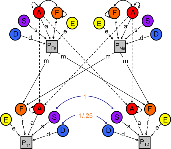
To evaluate the extent to which genetic and environmental influences on youth RB varied with neighbor RB, we made use of the NTFM. The NTFM (Figure 1) provides four pieces of information on which to base parameter estimates: the covariance between MZ twins, the covariance between DZ twins, the covariance between parents, and the covariance between parents and children (note: the classical twin model makes use of only the first two). This additional information allows us to estimate several parameters on top of standard genetic and non-shared environmental influences (all are defined in Table 1). We are able to disambiguate two general types of shared environmental influences: (a) those that create similarity between siblings, but not between parents and their children (termed S; e.g., exposure to common peers, school, and experiences of similar parenting across siblings) and (b) those that are passed via vertical “cultural transmission” between parents and their offspring (termed F; e.g., socioeconomic status, social mores). Comparing estimates of genetic effects (A), S, F, and nonshared environmental effects (E) across youth exposed to either lower or higher levels of neighbor RB (as divided at the median) thus allows us to explicitly evaluate which specific components of the shared environment varied with level of neighbor RB.
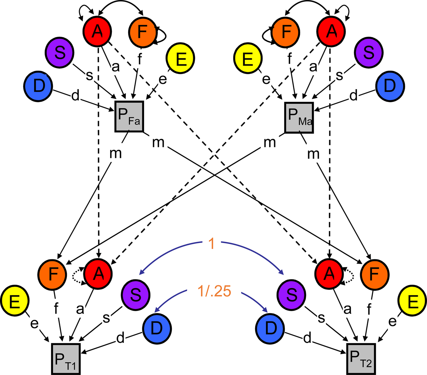
Figure 1. (Color online) Path diagram of the nuclear twin family model. Note: The variance in the phenotype (P) is parsed into that which is due to additive genetic effects (A), dominant genetic effects (D), sibling environmental influences (S), familial environmental influences (F; more specifically, m is estimated and f is fixed to 1), and nonshared environmental effects (E). (See Table 1 for definitions.) μ indexes primary phenotypic assortment (i.e., assortative mating) between the twin parents; w indexes the covariance between A and F. The staggered paths from parent A to twin A are fixed to .5. Paths are squared to estimate the proportion of variance accounted for. D, S, and F effects cannot be estimated simultaneously (only two of the three can be estimated); thus, D is not estimated in the current paper.
Table 1. Definitions of the parameters obtained Via twin modeling

Note: DZ, dizygotic; MZ, monozygotic.
Some parameters can be obtained only in the classical twin model (CTM), others can be obtained only in the nuclear twin family model (NTFM; see Figure 1), and others can be obtained in both models.
Just as important, however, the NTFM capitalizes on the individuation of the various types of shared environmental influences by directly estimating the covariance between vertical cultural transmission and genetic influences, otherwise known as passive gene–environment correlation (rGE; see w in Figure 1). Passive rGE refers to the fact that the environment parents provide to their biological children likely reflects the genetically influenced preferences/tendencies of the parent. And because parents also share genes with their biological children, the child's genes are then correlated with her environmental experiences (thereby mimicking shared environmental influences; Neiderhiser et al., Reference Neiderhiser, Reiss, Pedersen, Lichtenstein, Spotts, Hansson and Ellhammer2004). In our case, any moderation of shared environmental influences on youth RB by neighbor RB could actually reflect a moderated role for passive rGE, such that (for example) parents with a tendency toward RB themselves are both selecting into neighborhoods with like-minded people and passing on genes of risk for RB to their children. The NTFM overcomes this interpretative hurdle, allowing us to not only examine moderation of passive rGE effects, but also to more precisely model and interpret any moderation of shared environmental influences.
There are several assumptions undergirding the NTFM. First, although the model accommodates the possibility of assortative mating, it assumes that assortative mating stems from primary phenotypic assortment, in which mates choose each other based on phenotypic similarity, and does not allow for other forms of assortative mating (e.g., social homogamy, in which mates chose each other because of environmental similarity). Second, additive genetic and nonshared environmental estimates are assumed to influence all traits to some extent. However, because only four pieces of information (i.e., the covariance between MZ twins, the covariance between DZ twins, the covariance between parents, and the covariance between parents and children) are used to estimate model parameters, there is not enough information in the data to simultaneously estimate dominant genetic (D), S, and F effects (in addition to A and E). We are thus required to fix one of these estimates to zero. Given our specific questions, we focused specifically on the ASFE model herein, fixing D to zero in all models.
Specific analytic plan
We fitted the NTFM separately for families experiencing lower and higher levels of neighbor RB (divided at the median), and examined which model (ASFE, ASE, AFE, or AE) provided the best fit to the data at each level of neighbor RB. The ASFE model estimates additive genetic influences, sibling-level shared environmental influences, and family-level shared environmental influences and passive rGE. The ASE model drops family-level shared environmental influences, along with passive rGE, meaning that any shared environmental influences estimated in this model represent “legitimate” effects of the shared environment, unconfounded by passive rGE. The AFE model, by contrast, models all shared environmental influences as family-level effects/passive rGE. The AE model omits all shared environmental influences and passive rGE. We also ran a series of constraint models to directly evaluate whether we were able to constrain individual parameter estimates to be equal across the two neighbor RB groups and evaluated the change in model fit. Significant changes in fit would indicate that the parameter could not be constrained to be equal across higher and lower levels of neighbor RB.
To be consistent with the contagion model, however, the moderation of child RB by neighbor RB should also vary by proximity, such that etiologic moderation is enhanced in (or specific to) those twins who live closer to their neighbors. To evaluate whether proximity moderates the effect of high neighbor RB on child RB, we conducted two sets of analyses. First, we examined proximity to the nearest neighbor (operationalized here as <1km and 1–5km) as an etiologic moderator of child RB among those twins residing in neighborhoods with higher levels of neighbor RB (N = 410). An even stronger test of proximity would involve a two-moderator model, in which each moderator (average neighbor RB and proximity to neighbors) was allowed to simultaneously and synergistically moderate the etiology of a given outcome. Unfortunately, it is not yet possible to fit the NTFM within a two-moderator framework. We thus fitted a two-moderator GxE model using the classical twin model (Table 1; Purcell, Reference Purcell2002), which allowed us to directly test for the possibility of synergistic moderation by neighbor RB and proximity. In this model, the additive genetic variance component, for example, is represented as follows:
 $$\eqalign{\left(a + b_{neighborRB}M_{neighborRB} + b_{proximity}M_{proximity}\right.\cr \quad \left.+ b_{neighborRB \star proximity}M_{neighborRB}M_{proximity} \right)^2}$$
We were particularly interested in the neighbor RB*proximity, or synergistic, moderator estimates, which allowed us to directly evaluate whether the etiological moderation of child RB by neighbor RB varied with proximity to those neighbors. Should social contagion underlie the moderating effects of neighbor RB on twin RB, we would expect to see this effect enhanced in those twins who reside closer to their neighbors.
Analytic program
Mx (Neale, Boker, Xie, & Maes, Reference Neale, Boker, Xie and Maes2003) was used to fit the models to the data using Full-Information Maximum-Likelihood techniques. When fitting models to raw data, variances, covariances, and means are first freely estimated to get a baseline index of fit (minus twice the log-likelihood; –2lnL). The –2lnL in the unconstrained or “neighbor RB differences” model was then compared with that in the constrained or “no neighbor RB differences” model to compute the χ2 index of fit. Nonsignificant changes in χ2 indicate that the constrained model provided a better fit to the data. Model fit was also evaluated using four information theoretic indices that balance overall fit with model parsimony: the Akaike's Information Criterion (AIC; Akaike, Reference Akaike1987), the Bayesian Information Criteria (BIC; Raftery, Reference Raftery1995), the sample-size adjusted Bayesian Information Criterion (SABIC; Sclove, Reference Sclove1987), and the Deviance Information Criterion (DIC; Spiegelhalter, Best, Carlin, & Van Der Linde, Reference Spiegelhalter, Best, Carlin and Van Der Linde2002). The lowest or most negative AIC, BIC, SABIC, and DIC among a series of nested models is considered best. Because fit indices do not always agree (they place different values on parsimony, among other things), we reasoned that the better fitting model should yield lower or more negative values for at least three of the five fit indices described above.
Results
Paired samples t tests indicated that fathers were engaging in higher levels of RB relative to mothers (M = 12.88 and 11.96, respectively; p < .001). Independent samples t tests indicated that child RB also varied significantly across sex, such that boys evidenced higher rates of these behaviors than did girls (Cohen's d effect size was .23, p < .001). Child RB also varied by ethnicity and age, such that it was less common in White participants than in non-White participants (d = .34) and decreased slightly with child age (r = –.09, p < .01). Correlations conducted at the level of the individual neighbors indicated that neighbor RB was also more common in men than in women (r = .16, p < .001), more common in ethnic minority participants than in white participants (r = .22, p < .001), and decreased with age (r = –.15, p < .001).
The mean level of neighbor RB for all neighbors within 5km of the twins varied considerably across twin families (ranging from 11.00 [the floor] to 21.00; M = 12.76, SD = 1.07). Neighborhood-level descriptive statistics are presented in Table 2 (i.e., variables were aggregated within Census tracts or the 5km radius, as indicated, and then descriptive statistics were based on those aggregates; US Census data are presented at the level of the Census tract).
Table 2. Neighborhood-level descriptives

Note: Neighborhood is defined here via the 5km radius around a given twin family's residence. Averages within those neighborhoods are presented in the text. Mean household income by neighborhoods corresponds to roughly $35,000/yr and ranged from <$10,000 (coded 1) to >$50,000 (coded 10). The average level of educational attainment by neighborhood (4.49) corresponds to “some college,” and ranged from “some high school” (coded 2) to “graduate degree” (coded 7). To examine the proportion of neighborhood informants in a given neighborhood who were male, ethnic minority, unmarried, and/or had children, those variables were each dummy-coded (0, 1). The mean neighborhood contained neighbor informants that were 33% male, 18% ethnic minority, 38% unmarried, and 82% parents; however, the full range was represented (e.g., in some neighborhoods, 0% of the participants were male, whereas in other neighborhoods, all participants were male).
*The Census-level neighborhood data were computed via Census tracts (the unit used most often when examining US Census data).
**Given that all families were recruited from 2008 onwards, we focused on the 2008–2012 Census data here. A handful of families (n = 80) resided in Census tracts that appear to have “gentrified” somewhat over the intake recruitment period (e.g., the tract was above the poverty cut-point of 10.5% according to the 2005–2009 Census data available at the time of recruitment, but not according to the 2008–2012 data).
Parents’ own RB was modestly correlated with teacher reports of their children's RB (r = .10 for mothers and .13 for father, both p < .01), indicating that, as expected, parental behavior predicts child behavior and does so even across different informants. There was also evidence of modest assortative mating for RB (r = .17, p < .001), such that parents were more similar in their RB than would be expected by chance. Neighbor RB was also modestly correlated with twin, mother, and father RB (r = .12, .14, and .08, respectively).
We also computed intraclass correlations, separately by zygosity and level of neighbor RB (divided at the median). Twin RB data were double-entered for these particular analyses, in keeping with standard practices. Results indicated that the MZ correlation was roughly double that of the DZ correlation in neighborhoods with less neighbor RB (r = .60 and .25, respectively; z = 3.78, p < .001). Such results suggest that child RB may be largely genetic in origin in the absence of exposure to high levels of neighbor RB. As neighbor RB increased, however, so too did the DZ correlation (r = .45; z = 2.12, p = .03), so much so that the MZ (r = .59) and DZ correlations were statistically equivalent (z = 1.53, p = .13) with exposure to higher neighbor RB. Such results point to prominent shared environmental influences in these neighborhoods.
GxE analyses
We fitted the NTFM to the twin family RB data separately by level of neighbor RB and then constrained estimates to be equal across level of neighbor RB. The fully unconstrained ASFE model fitted the data well (–2lnL = 7,465.96 on 2,662 df; AIC = 2,141.96; BIC = –5,216.44; SABIC = –989.65; DIC = –2,770.23) and uniformly better than the fully constrained ASFE model, in which all parameter estimates were constrained across lower and higher neighbor RB groups (–2lnL = 7,516.71 on 2,668 df, Δχ2 = 50.75 on 6 df, p < .001; AIC = 2,180.71; BIC = –5,211.24; SABIC = –974.92; DIC = –2,759.51). Such findings indicate that the etiology of youth RB does indeed vary according to the level of neighbor RB.
Parameter estimates from the fully unconstrained ASFE model are presented in Table 3. As seen there, shared sibling environmental influences (S) on youth RB were negligible at lower levels of neighbor RB but significant and moderate in magnitude at higher levels of neighbor RB. By contrast, family environmental or vertical cultural F and passive rGE effects were small and insignificant at higher levels of neighbor RB but were significant at lower levels of neighbor RB. Genetic influences on youth RB were moderate-to-large in magnitude, regardless of the level of neighbor RB.
Table 3. Unstandardized nuclear twin family design heritability estimates for child RB, by level of RB in neighbors residing within 5km of the twin family

Note: A, additive genetic behavior; E, environmental influences shared between siblings; F, family environmental influence; RB, nonaggressive antisocial behavior; S, nonshared environmental influences.
* and bold font indicate that the parameter is significantly larger than zero at p < .05. The same lowercase letter indicates that the estimated parameters differ significantly from one another at p < .05.
To confirm these impressions, we evaluated which NTFM (i.e., ASFE, AFE, ASE, or AE) provided the best fit to the RB data at lower and higher levels of neighbor RB, respectively. Model fit results are presented in Table 4. As seen there, the AFE model provided the best fit to the data in lower RB neighborhoods, whereas the ASE model provided the best fit to the data in higher RB neighborhoods. Such results confirmed our earlier impressions, namely that the types of shared environmental influences contributing to child RB vary with their exposure to neighbor RB. Additional constraint analyses for each parameter estimate (Table 3; specific model fits available upon request) further revealed that neither A (at least in the best-fitting models) nor S could be individually constrained across neighborhood type without a significant decrement in fit.
Table 4. NTFM fit indices for nonaggressive RB, separately by level of neighbor RB

Note: Additive genetic, environmental influences shared between siblings, family environmental influences, and nonshared environmental influences are represented with A, S, F, and E, respectively; χ2, change in chi-square relative to the full ASFE model (*indicates a significant change at p < .05). The best fitting model for a given set of analyses is highlighted in bold font, and is indicated by a nonsignificant change in χ2 relative to the linear ACE moderation model and/or the lowest or most negative AIC (Akaike's Information Criterion), BIC (Bayesian Information Criterion), SABIC (sample size adjusted Bayesian Information Criterion), and DIC (Deviance Information Criterion) values for at least 3 of the 5 fit indices.
Does this effect vary with the twins’ proximity to their neighbors?
To evaluate whether proximity moderates the effect of high neighbor RB on child RB, we first examined proximity to the nearest neighbor (operationalized here as <1km and 1–5km) as an etiologic moderator of child RB using the NTFM, restricting our analyses to those twins residing in neighborhoods with higher levels of neighbor RB (N = 410). The fully unconstrained nuclear twin family ASFE model fitted the data well (–2lnL = 3,681.71 on 1,241 df; AIC = 1,199.71; BIC = –1,875.30; SABIC = 93.58; DIC = –734.89) and better than the fully constrained ASFE model, in which all parameter estimates were constrained across lower and higher proximity groups (–2lnL = 3,703.91 on 1,247 df, Δχ2 = 22.20 on 6 df, p = .001; AIC = 1,209.91; BIC = –1,882.16; SABIC = 96.24; DIC = –736.25). Parameter estimates are presented in Table 5. Additional constraint analyses (also indicated in Table 5; specific model fits available upon request) further revealed that none of the individual parameter estimates (A, S, F, or E) could be individually constrained across proximity without a significant decrement in fit.
Table 5. Unstandardized nuclear twin family design heritability estimates for child RB in those exposed to higher levels of neighbor RB, separately by proximity to neighbors

Note: RB refers to nonaggressive antisocial behavior. Additive genetic, environmental influences shared between siblings, family environmental influences, and nonshared environmental influences are represented with A, S, F, and E, respectively. * and bold font indicate that the parameter is significantly larger than zero at p < .05. The same lowercase letter indicates that the estimated parameters differ significantly from one another at p < .05.
Second, because it is not yet possible to fit the NTFM within a two-moderator framework (in which each moderator simultaneously and synergistically moderates the etiology of a given outcome within a NTFM design), we also fitted a two-moderator GxE model examining proximity and neighbor RB as simultaneous etiologic moderators of child RB using the classical twin model (Table 1; Purcell, Reference Purcell2002). We were specifically interested in the proximity-X-neighbor RB or interactive moderator estimates, which evaluated whether the etiological moderation of child RB by neighbor RB varied with proximity to those neighbors. Two of the three synergistic moderators (A and E, estimated at .86 and –.30, respectively) were significantly larger than zero in the full model. The synergistic shared environmental moderator, although large in magnitude (–.78), was only marginally significant. A radar plot of the estimates is presented in Figure 2. When viewed alongside the NTFM constraint models for proximity, these results collectively suggest that the increase in S and the decrease in A seen in youth whose neighbors engage in higher levels of RB is largely confined to those twins who reside in closer proximity to those neighbors.
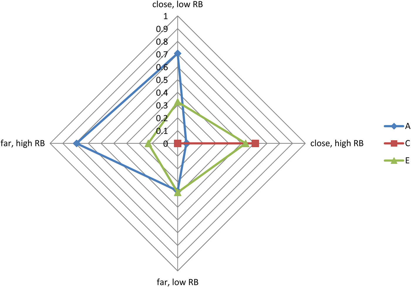
Figure 2. (Color online) Radar plot of the classical twin two-moderator model.
Post-hoc analyses
What specific element of neighbor RB is driving the etiologic moderation of youth RB?
The findings given here are agnostic with regard to the specific elements of neighbor RB driving the moderation. In an attempt to fill this gap, we evaluated the specific items composing the neighbor RB scale and selected those assessing acts with visible consequences for the broader community. These included littering and vandalism (both of which leave blight in their wake), selling drugs (a crime that can and does happen in front of neighborhood youth), and frequent joblessness (resulting in increased numbers of unemployed adults in the neighborhood). We then examined which of these specific aspects of the neighbor RB scale uniquely predicted child RB via a series of two-level MLM random effects regression models (to adjust for the nonindependence within families). Results pointed squarely to joblessness as the element of neighbor RB that most meaningfully predicts youth RB (estimates [standard error] were .16 [.16], p = .33, for crime, –.20 [.24], p = .39, for blight, and .27 [.12], p = .02, for joblessness).
Given these results, we then examined whether frequent joblessness in the twins’ neighbors also moderated the etiology of youth RB in our primary NTFM framework. As with neighbor RB, the fully unconstrained ASFE model fitted the data well (–2lnL = 7,486.54 on 2,662 df; AIC = 2,162.54; BIC = –5,206.15; SABIC = –979.36; DIC = –2,759.94) and better than the fully constrained ASFE model, in which all parameter estimates were constrained across lower and higher joblessness (–2lnL = 7,516.71 on 2,668 df; Δχ2 = 30.17 on 6 df, p < .001; AIC = 2,180.71; BIC = –5,211.24; SABIC = –974.92; DIC = –2,759.51). Such findings indicate that the etiology of youth RB does indeed vary according to the level of neighbor joblessness. We then evaluated which model (i.e., ASFE, AFE, ASE, or AE) provided the best fit to the child RB data at lower and higher levels of neighbor joblessness, respectively. Results are presented in Supplementary Tables 1 and 2. As seen there, the results were very much in keeping with those for neighbor RB more broadly, in that the AFE model provided the best fit to the data in the presence of lower levels of joblessness and the ASE model provided the better fit to the data in the presence of higher levels of joblessness. Moreover, there was at least some evidence of a decrease in genetic influences on child RB with increasing levels of neighbor joblessness.
Discussion
The primary goal of the current study was to evaluate whether and how neighbor RB might shape the etiology of child RB, thereby providing an early test of social contagion as an element of prior GxE findings. Phenotypic correlations indicated that nonaggressive RB appeared to cluster somewhat by neighborhood, such that many of those residing in the same neighborhood (e.g., neighbors, twins, mothers, fathers) were more similar in their RB than would be expected by chance. Nuclear twin family GxE analyses indicated that sibling-level shared environmental influences on child RB increased many-fold and family-level shared environmental and genetic influences on RB simultaneously decreased (if somewhat less robustly) in the presence of higher levels of neighbor RB. Moreover, this etiologic moderation was accentuated when proximity was also taken into account, such that child RB was almost entirely a function of sibling-level shared and nonshared environmental influences in those residing close to neighbors with high levels of RB, and largely genetic in origin in those residing either farther from these neighbors or in those residing near neighbors engaging in low levels of RB. The specific element of neighbor RB that appeared to drive these effects was frequent joblessness.
How do we make sense of these results, and specifically the similarity in etiology across those residing farther from high RB neighbors and those residing near low RB neighbors (as can be seen in Figure 2)? One hypothesis is that the genetic and nonshared environmental etiology of youth RB in those three contexts may represent something akin to its “standard” etiology and that close proximity to high RB neighbors provides such a strong social push for youth RB that it obviates the importance of these otherwise standard genetic contributions. This sort of bioecological GxE has also been reported for IQ, such that genetic influences on IQ are important primarily in middle- and upper-class families. In low-income families, by contrast, environmental influences predominate. In short, it may well be the case that the stressors associated with impoverishment interfere with normative intellectual/behavioral development, and do so regardless of the child's genetic predispositions.
The importance of significant sibling-level environmental influences also constructively replicates prior work from our lab (Burt & Klump, Reference Burt and Klump2012). Burt and Klump (Reference Burt and Klump2012) fitted the nuclear twin family model to child RB data from the population-based arm of our child twin study. Results revealed that sibling-level environmental influences were an important contributor to child RB (accounting for ~20% of its overall variance and nearly all of its shared environmental variance), whereas vertical cultural transmission made minimal contributions. The current results were generally consistent with these prior results, in that sibling-level environmental influences appeared to both contribute to child RB and to account for much of the change in shared environmental influences found in our GxE models. Vertical cultural transmission effects, on the other hand, were relatively small in magnitude. In short, the current results bolster prior work indicating that the sibling-level environment constitutes a critical component of the shared environmental influences on child RB.
Finally, our results indicated that neighbors’ unemployment, rather than elements of adult RB that would increase crime or blight, are particularly important for understanding these effects. Although it is not entirely clear how to understand these results, one plausible explanation is that unemployment acts as an indirect proxy for neighborhood social characteristics such as residential instability, low collective efficacy, or the willingness of neighborhood residents to intervene in local problems (Raudenbush & Sampson, Reference Raudenbush and Sampson1999). Living in neighborhoods with these sorts of social characteristics has been shown to sharply lower expectations for shared child control (Sampson, Morenoff, & Earls, Reference Sampson, Morenoff and Earls1999) and increased antisocial behaviors of children at school entry (Odgers et al., Reference Odgers, Moffitt, Tach, Sampson, Taylor, Matthews and Caspi2009). Future work should examine neighborhood social characteristics directly to evaluate whether and how they might drive the effects observed here.
Limitations
There are several limitations to the current study. First, the pattern of etiologic moderation observed for neighbor RB was quite similar to that observed for neighborhood poverty (Burt et al., Reference Burt, Klump, Gorman-Smith and Neiderhiser2016). It thus remains unclear whether these results would persist once we controlled for the association (r = .31) between neighbor RB and neighborhood poverty. To evaluate this question, we regressed neighborhood poverty onto neighbor RB and examined the residual as our etiologic moderator. Overall parameter estimates were nearly identical to those reported in Table 3 (r = .98). The mean difference in parameter estimates was .038, with a range of .00 to .06. Moreover, the S parameter estimate (.09) was not significant at low levels of the neighbor RB residual, whereas the F parameter estimate (.05) was not significant at high levels of neighbor RB. In short, our results are not a function of neighborhood poverty per se.
Second, although the incorporation of parent data serves to dramatically increase the statistical power of twin data (Heath, Kender, Eaves, & Markell, Reference Heath, Kender, Eaves and Markell1985), our sample size of 847 families is considered only moderately sized for GxE analyses. Moreover, because our analyses were already complicated, we regressed sex out of twin RB before analysis. Future studies should thus evaluate joint moderation by sex. Third, given the core role of development in the etiology of conduct problems (Burt & Neiderhiser, Reference Burt and Neiderhiser2009), the current results should be considered specific to middle childhood and not be applied to other developmental periods. Fourth, because analyses were conducted on a sample that resided in or near modestly to severely disadvantaged neighborhood contexts, our findings are specific to this population, and do not apply to other sorts of populations (e.g., epidemiological, case control).
Next, although our neighborhood informant sample is large and typically includes several participants per neighborhood, it is nevertheless unclear whether participating neighbors were representative of adults in their neighborhoods. To preliminarily evaluate this issue, we have examined whether official Census data on mean ethnicity in each Census tract predicted mean neighbor self-reports of ethnicity clustered using those same Census tracts. The two were highly correlated .68 (p < .001). Moreover, in those Census tracts in which all of our neighborhood informant participants identified as white, the mean proportion of white individuals was 89.0%, whereas the mean proportion of black individuals was 6.9%. In short, there is evidence, albeit limited, to suggest that participants in our neighborhood informant sample are indeed representative of their overall neighborhoods. However, future work should explore this issue in more depth.
Finally, to maximize our sample size for our power-intensive constraint models, we made use of a large geographic radius in our analyses, a less than ideal approach for studies of neighbors/neighborhoods. Fortunately, our results persisted when examining much smaller geographic areas (when examining the twin family's nearest neighbor or their Census tract). Because our analyses further suggested that the effects of neighbors were exacerbated by physical proximity, however, future studies of social contagion GxE should be mindful of geographic and/or social proximity to others.
Conclusions
The current results indicate that neighborhood contexts, including the behaviors of neighbors in those contexts, appear to exert rather profound effects on the etiology of youth nonaggressive RB. Shared environmental influences that create similarity between siblings are significantly more potent in the presence of nonaggressive RB in families’ neighbors. These sibling-level environmental influences are thought to include a broad array of environmental experiences, including those more proximal to the child (e.g., parenting, peers) and those more distal (e.g., schools, child-relevant neighborhood characteristics). Genetic influences, by contrast, are significantly lower in these particular contexts, and this is especially the case when the twins live in close proximity to neighbors reporting higher levels of RB. Shared environmental influences that create family-wide similarity (i.e., between parents and their children and between siblings; e.g., SES) and passive rGE are similarly lower in the presence of higher neighbor RB.
These findings of etiologic moderation of children's RB by the RB behavior of their neighbors have several broad implications. On the one hand, they further legitimize the bioecological model of GxE identified herein, in that findings of environmental moderation represent actual environmental influences that increase in importance with proximity to relevant neighbor behaviors, and specifically, neighbor joblessness. This is especially important for our general understanding of GxE because most GxE studies conducted to date have focused on diathesis-stress GxE (Burt, Reference Burt2011), a fundamentally different model. Under the diathesis-stress model, GxE would manifest as stronger genetic effects in the presence of environmental risk. Put differently, the diathesis-stress model would predict absolute (or unstandardized) increases in genetic influences with increasing environmental risk exposure. There are no clear predictions for environmental influences on the outcome. Under the bioecological model, by contrast, deleterious environments are thought to amplify (shared) environmental influences, whereas genetic influences are more important under normative environmental conditions. In this case, the model would specifically predict absolute increases in environmental influences with increasing environmental risk exposure. Genetic influences on the outcome would be expected to decrease. This is precisely the pattern of GxE observed here.
Although such results thus provide clear evidence for the bioecological model of GxE, they also circumstantially point toward the need for a more meaningful shift in our consideration of the processes driving GxE, in that bioecological GxE processes should perhaps be considered an example of the phenomenon of contagion or “spread.” Much in the same way that viruses and bacteria spread with physical proximity, so too do RB behaviors. By contrast, individual and familial susceptibility to these RB behaviors matter considerably more in the absence of those “contagious” behaviors. Future research should explore this possibility in more depth.
Supplementary Material
To view the supplementary material for this article, please visit https://doi.org/10.1017/S0954579418000366.